A&A 439, 887-900 (2005)
DOI: 10.1051/0004-6361:20041964
A. Pollo1 - B. Meneux2 - L. Guzzo1 - O. Le Fèvre2 - J. Blaizot2 - A. Cappi3 - A. Iovino4 - C. Marinoni2 - H. J. McCracken5,6D. Bottini7 - B. Garilli7 - V. Le Brun2 - D. Maccagni7 - J. P. Picat8 - R. Scaramella9 - M. Scodeggio7 - L. Tresse2 - G. Vettolani10 - A. Zanichelli10 - C. Adami2 - M. Arnaboldi13 - S. Arnouts2 - S. Bardelli3 - M. Bolzonella3 - S. Charlot5,11 - P. Ciliegi10 - T. Contini8 - S. Foucaud7 - P. Franzetti7 - I. Gavignaud8 - O. Ilbert2 - B. Marano12 - G. Mathez8 - A. Mazure2 - R. Merighi3 - S. Paltani2 - R. Pellò8 - L. Pozzetti3 - M. Radovich13 - G. Zamorani3 - E. Zucca3 - M. Bondi10 - A. Bongiorno3 - G. Busarello13 - L. Gregorini10 - F. Lamareille8 - Y. Mellier5,6 - P. Merluzzi13 - V. Ripepi13 - D. Rizzo8
1 -
INAF - Osservatorio Astronomico di Brera, via Bianchi 46, Merate (LC),
Italy
2 -
Laboratoire d'Astrophysique de Marseille, UMR 6110 CNRS, Université
de Provence, Traverse du Siphon-Les trois Lucs, 13012 Marseille, France
3 -
INAF - Osservatorio Astronomico di Bologna, via Ranzani 1, 40127 Bologna, Italy
4 -
INAF - Osservatorio Astronomico di Brera, via Brera, 20121 Milan, Italy
5 -
Institut d'Astrophysique de Paris, UMR 7095, 98bis Bd. Arago, 75014 Paris, France
6 -
Observatoire de Paris, LERMA, UMR 8112, 61 Av. de l'Observatoire, 75014 Paris, France
7 -
IASF - INAF, 20133 Milano, Italy
8 -
Laboratoire d'Astrophysique - Observatoire Midi-Pyrénées, 31400 Toulouse, France
9 -
INAF - Osservatorio Astronomico di Roma, Italy
10 -
INAF - Istituto di Radio-Astronomia, Bologna, Italy
11 -
Max-Planck-Institut für Astrophysik, 85741 Garching, Germany
12 -
Università di Bologna, Departimento di Astronomia, via Ranzani 1, 40127 Bologna, Italy
13 -
INAF - Osservatorio Astronomico di Capodimonte, via Moiariello 16, 80131 Napoli, Italy
Received 6 September 2004 / Accepted 10 March 2005
Abstract
We present
a detailed description
of
the methods used
to compute the three-dimensional two-point galaxy correlation
function in the VIMOS-VLT deep survey (VVDS).
We investigate how
instrumental selection effects and observational biases affect
the measurements and identify the methods to correct for them. We
quantify the accuracy of our
corrections using an
ensemble of 50 mock galaxy surveys generated with the GalICS
semi-analytic model of galaxy formation which
incorporate the
selection biases and tiling strategy
of the real data.
We demonstrate that we are able to recover the
real-space two-point correlation function ![]() and the projected correlation function
and the projected correlation function
![]() to an accuracy better than 10%
on scales larger than 1 h-1 Mpc
with the sampling strategy used for the first epoch
VVDS data.
The large number of simulated surveys allows us to provide a reliable
estimate of the cosmic variance on the measurements of
the correlation length r0 at
to an accuracy better than 10%
on scales larger than 1 h-1 Mpc
with the sampling strategy used for the first epoch
VVDS data.
The large number of simulated surveys allows us to provide a reliable
estimate of the cosmic variance on the measurements of
the correlation length r0 at ![]() ,
of about 15-20%
for the first epoch VVDS observation
while any residual systematic effect in the measurements of r0 is always
below
,
of about 15-20%
for the first epoch VVDS observation
while any residual systematic effect in the measurements of r0 is always
below ![]() .
The
error estimation and measurement techniques outlined in this paper
are being used in several parallel studies which investigate in
detail the clustering properties of galaxies in the VVDS.
.
The
error estimation and measurement techniques outlined in this paper
are being used in several parallel studies which investigate in
detail the clustering properties of galaxies in the VVDS.
Key words: cosmology: large scale structure of Universe - methods: statistical - galaxies: evolution - surveys
The VIMOS VLT Deep Survey (VVDS, Le Fèvre et al. 2005a) is dedicated to
study the evolution of galaxies and large scale structure to ![]() with a significant fraction of galaxies reaching
with a significant fraction of galaxies reaching ![]() .
The VVDS
spectroscopic survey is performed with the VIMOS spectrograph at the European
Southern Observatory Very Large Telescope
and
complemented with multi-color BVRI imaging
data obtained at the CFHT telescope (McCracken et al. 2003; Le Fèvre et al. 2004).
The complete survey will consist of four fields of
.
The VVDS
spectroscopic survey is performed with the VIMOS spectrograph at the European
Southern Observatory Very Large Telescope
and
complemented with multi-color BVRI imaging
data obtained at the CFHT telescope (McCracken et al. 2003; Le Fèvre et al. 2004).
The complete survey will consist of four fields of ![]() by
by
![]() each, with multi-band photometry coverage in the BVRI (and
partly UJK) bands. Multi-object spectroscopy down to
IAB = 22.5is being obtained over the four fields ("VVDS Wide''), with a deeper
area of 1.5 deg2 in the VVDS-02h and in the Chandra Deep Field
South (VVDS-CDFS) covered to
IAB = 24 ("VVDS Deep''). The first
epoch VVDS data consist of more than 11 000 spectra obtained in the
VVDS-Deep fields (Le Fèvre et al. 2005a).
each, with multi-band photometry coverage in the BVRI (and
partly UJK) bands. Multi-object spectroscopy down to
IAB = 22.5is being obtained over the four fields ("VVDS Wide''), with a deeper
area of 1.5 deg2 in the VVDS-02h and in the Chandra Deep Field
South (VVDS-CDFS) covered to
IAB = 24 ("VVDS Deep''). The first
epoch VVDS data consist of more than 11 000 spectra obtained in the
VVDS-Deep fields (Le Fèvre et al. 2005a).
One of the key science goals of the VVDS is to measure the evolution of
galaxy clustering from the present epoch up to ![]() .
The
simplest statistic used for this analysis is the spatial two-point
correlation function
.
The
simplest statistic used for this analysis is the spatial two-point
correlation function ![]() and its variants,
(e.g. Peebles 1980), i.e. the second moment of the galaxy
distribution. Given the geometry and selection function of galaxy
surveys, however, the practical estimation of
and its variants,
(e.g. Peebles 1980), i.e. the second moment of the galaxy
distribution. Given the geometry and selection function of galaxy
surveys, however, the practical estimation of ![]() from the actual
data is not straightforward. Edge effects, sampling inhomogeneities and
selection effects all introduce different biases that hamper the
survey's ability to estimate the true underlying clustering process.
Moreover, intrinsic systematic uncertainties due to the limited size of
the volume of the Universe explored ("cosmic variance'') need to be
accounted for when computing realistic error bars on the measured
correlation values.
from the actual
data is not straightforward. Edge effects, sampling inhomogeneities and
selection effects all introduce different biases that hamper the
survey's ability to estimate the true underlying clustering process.
Moreover, intrinsic systematic uncertainties due to the limited size of
the volume of the Universe explored ("cosmic variance'') need to be
accounted for when computing realistic error bars on the measured
correlation values.
The aim of this paper is to present a comprehensive description of the biases specific to the VVDS, along with the methods we developed to correct for them. The strategy we adopt relies on the construction of realistic "pre-observation'' mock catalogs using the MoMaF software (Blaizot et al. 2005) and the GalICS hybrid model for galaxy formation (Hatton et al. 2003). We then observe these mock catalogs, by mimicking the relevant observational selections and biases. Comparing original and observed mock surveys allows us to (i) quantitatively understand the impact of the different biases inherent to the VVDS data on clustering estimates, and (ii) to explore and validate methods that allow us to recover the original signal. This strategy is possible because GalICS predictions have been shown to agree fairly well with a wide range of observations (e.g. Hatton et al. 2003; Blaizot et al. 2004), and is thus expected to yield catalogs realistic enough to carry out a convincing consistency check. Because our mock catalogs contain realistic clustering properties, we can also use them to predict the cosmic variance amplitude in order to compute realistic errors on the clustering estimates we will perform on the real data.
The paper is organized as follows. In Sect. 2 we discuss the
different kind of biases expected in the current VVDS first-epoch data.
In Sect. 3 we discuss the construction of mock VVDS catalogs from the
GalICS/MoMaf simulations which assume a flat Cold Dark Matter model
with
![]() ,
,
![]() and h = 0.667.
In Sect. 4 we present the definitions of the
two-point correlation functions. Then, in Sect. 5 we discuss the details of
the error measurement strategy when applied
to VVDS. In Sect. 6 we show how the measured
two-point correlation function is affected by the features particular
to our survey and we discuss the methods developed to
correct for these biases and properly estimate the correlation function
and h = 0.667.
In Sect. 4 we present the definitions of the
two-point correlation functions. Then, in Sect. 5 we discuss the details of
the error measurement strategy when applied
to VVDS. In Sect. 6 we show how the measured
two-point correlation function is affected by the features particular
to our survey and we discuss the methods developed to
correct for these biases and properly estimate the correlation function
![]() ,
its projection
,
its projection
![]() ,
and the correlation length
r0 and slope
,
and the correlation length
r0 and slope ![]() ,
as a function of redshift.
Section 7 summarizes our results.
,
as a function of redshift.
Section 7 summarizes our results.
The first epoch spectra of the VVDS-Deep
collected during the 2002 and 2003 campaigns
are concentrated within the 02h deep field, and the CDFS
(Le Fèvre et al. 2005a).
First epoch spectra have been collected for galaxies down to
![]() in the
0.61 sq degree
sub-area of the VVDS-02h field and a region of
in the
0.61 sq degree
sub-area of the VVDS-02h field and a region of
![]() sq arcmin centered on the Chandra Deep Field South (CDFS,
Giacconi et al. 2002).
The VVDS First Epoch data geometrical lay-out,
sampling rate and incompleteness are used
as a reference benchmark in this paper.
sq arcmin centered on the Chandra Deep Field South (CDFS,
Giacconi et al. 2002).
The VVDS First Epoch data geometrical lay-out,
sampling rate and incompleteness are used
as a reference benchmark in this paper.
![\begin{figure}
\par\includegraphics[width=7.8cm,clip]{1964fi01.ps} \end{figure}](/articles/aa/full/2005/33/aa1964-04/img21.gif) |
Figure 1: Lay-out of the VIMOS field of view. INVAR masks with laser-cut slits are placed on the focal plane within the four rectangular areas ("VIMOS channels''). |
| Open with DEXTER | |
![\begin{figure}
\par\includegraphics[width=7.3cm,clip]{1964fi02.ps}\hspace*{7mm}
\includegraphics[width=7.3cm,clip]{1964fi03.ps} \end{figure}](/articles/aa/full/2005/33/aa1964-04/img22.gif) |
Figure 2:
Galaxy
distribution in a mock VVDS-02h catalog, constructed using the
GalICS simulations with the same lay-out as the 20 observed
pointings in the actual first-epoch VVDS field and applying the full
range of selection effects present in the data, as e.g. the
photometric mask. The left panel shows the parent photometric
field, including all objects with
|
| Open with DEXTER | |
A number of factors, both in the parent photometric catalog from which the target galaxies are selected and in the way the spectroscopic observations are carried out, contribute to create selection effects that bias any estimate of galaxy clustering if not properly accounted for.
![\begin{figure}
\par\includegraphics[width=7.5cm,clip]{1964fi04.ps} \end{figure}](/articles/aa/full/2005/33/aa1964-04/img24.gif) |
Figure 3: Spectroscopic targets (filled circles) selected in one of the four VIMOS quadrants from a complete VVDS mock photometric sample (open circles). Note how the optimization software tends to select spectroscopic targets aligned along horizontal rows, while, clearly, very close pairs are not observed. Typically, however, 4 independent observations are conducted on the same area, each with a similar target layout, but shifted by a few arcminutes. This significantly reduces both the alignment and proximity effects. The residual bias is then further corrected by the weighting scheme discussed in Sect. 4. Overall, the four passes produce a typical sampling rate of one galaxy in four. |
| Open with DEXTER | |
The only way to understand the relative importance of the selection biases discussed above and test possible correction schemes is to create and analyze realistic simulations of our survey. Provided these simulations are realistic enough, they allow us (1) to understand quantitatively the magnitude of observational biases on the final statistical quantities to be measured, and (2) to estimate realistic errors that include cosmic variance. Both these points require that mock observations contain a spatial distribution of galaxies consistent with VVDS observations - so as to measure clustering and cosmic variance - along with realistic photometric and physical properties of simulated galaxies - so as to mimic selection effects. The GalICS model for galaxy formation (Hatton et al. 2003) along with the MoMaF mock observing tool (Blaizot et al. 2005) fulfill these requirements and we thus use them to build "pre-observation'' catalogs that we then "observe'' by progressively adding all the VVDS observational biases and selections.
In this section, we first describe the GalICS simulation that we use, before discussing how we build simulated VVDS observations that account for all identified biases.
GalICS (for Galaxies In Cosmological Simulations, see Hatton et al. 2003) is a model of hierarchical galaxy formation which combines high resolution cosmological simulations to describe the dark matter content of the Universe with semi-analytic prescriptions to deal with the baryonic matter.
The cosmological N-body simulation we refer to throughout this paper
assumes a flat cold dark matter model with a cosmological constant
(
![]() ,
,
![]() ). The simulated volume
is a cube of side
). The simulated volume
is a cube of side
![]() Mpc, with h = 0.667,
containing 2563 particles of mass
Mpc, with h = 0.667,
containing 2563 particles of mass
![]()
![]() ,
with a smoothing length of 29.29 kpc. The power spectrum was set in
agreement with the present-day abundance of rich clusters (
,
with a smoothing length of 29.29 kpc. The power spectrum was set in
agreement with the present-day abundance of rich clusters (
![]() ,
from Eke et al. 1996), and the DM density field was evolved from z=35.59 to z=0,
outputting 100 snapshots spaced logarithmically in the expansion factor.
,
from Eke et al. 1996), and the DM density field was evolved from z=35.59 to z=0,
outputting 100 snapshots spaced logarithmically in the expansion factor.
GalICS builds galaxies from this simulation in two steps. First, halos of DM containing more than 20 particles are identified in each snapshot using a friend-of-friend algorithm. Their merging history trees are then computed following the constituent particles from one output to the next. Second, baryons are evolved within these halo merging history trees according to a set of semi-analytic prescriptions that aim to account for e.g. heating and cooling of the gas within halos, star formation and its feedback on the environment, stellar population evolution and metal enrichment, formation of spheroids through galaxy mergers or disc instabilities.
Three main points make GalICS particularly suitable for this study. First, this model yields a wide range of predictions, among which luminosities (in many bands from the UV to the sub-mm), physical properties (such as sizes of galaxies), and the positions of galaxies within the simulation snapshots. Second, these properties have been shown to be in a rather good agreement with various observations (e.g. Hatton et al. 2003; Blaizot et al. 2004). Third, mock observations are readily available from the GalICS Project's web-page![]() . These mock observations include 50 catalogs of
. These mock observations include 50 catalogs of ![]() sq deg that contain all the information we need in this study: apparent magnitudes in the BVRI filters used at the CFHT, apparent sizes of the galaxies, angular coordinates in the mock sky, and redshifts.
sq deg that contain all the information we need in this study: apparent magnitudes in the BVRI filters used at the CFHT, apparent sizes of the galaxies, angular coordinates in the mock sky, and redshifts.
Before using GalICS mock samples, it is useful to state their limitations (see however Blaizot et al. 2005, for a thorough description of these). There are mainly three shortcomings to mock catalogs made using GalICS. First, because of the finite mass resolution of the root simulation, faint galaxies are not well described, or even missed when they lie in unresolved haloes. This is not an issue for the present study, however, because the VVDS detection limit is brighter than GalICS's resolution. Second, because mock catalogs are built from a simulation of a finite volume, they involve replications of this volume, along and perpendicular to the line of sight. These replications lead to some negative bias in the correlation functions, of at most ![]() 10%. This is not a concern in this paper, because we just need an approximate match with the observed data in order to perform an internal consistency check. GalICS catalogs do provide an adequate match. Third, the mock catalogs do not describe density fluctuations on scales larger than the size of the simulated volume (
10%. This is not a concern in this paper, because we just need an approximate match with the observed data in order to perform an internal consistency check. GalICS catalogs do provide an adequate match. Third, the mock catalogs do not describe density fluctuations on scales larger than the size of the simulated volume (![]() 100 h-1 Mpc). This implies that cosmic variance estimates are likely to be under-estimated if the volume probed by a mock catalog is larger than the simulated volume. This under-estimate, however, depends on the galaxy population considered: it will be large for rare objects and small for "normal'' galaxies. In other words, because cosmic variance is basically given by the integral of the correlation function over the survey, the error on the estimated cosmic variance depends on how much of this integral we miss, that is, on how strongly the studied galaxies are clustered. From Fig. 9, it can be seen that the size of the simulation is enough for this under-estimate to be small at the scales we consider (i.e. from 0.1 to 10 h-1 Mpc). The dispersion found among the 50 GalICS cones is thus expected to be a good estimate of cosmic variance.
The mean number of galaxies with
17.5 < IAB < 24 in the artificial catalogs is 77 396. The average redshift
distribution of these 50 cones is shown in Fig. 4, along with
the VVDS first epoch N(z) (Le Fèvre et al. 2005a).
100 h-1 Mpc). This implies that cosmic variance estimates are likely to be under-estimated if the volume probed by a mock catalog is larger than the simulated volume. This under-estimate, however, depends on the galaxy population considered: it will be large for rare objects and small for "normal'' galaxies. In other words, because cosmic variance is basically given by the integral of the correlation function over the survey, the error on the estimated cosmic variance depends on how much of this integral we miss, that is, on how strongly the studied galaxies are clustered. From Fig. 9, it can be seen that the size of the simulation is enough for this under-estimate to be small at the scales we consider (i.e. from 0.1 to 10 h-1 Mpc). The dispersion found among the 50 GalICS cones is thus expected to be a good estimate of cosmic variance.
The mean number of galaxies with
17.5 < IAB < 24 in the artificial catalogs is 77 396. The average redshift
distribution of these 50 cones is shown in Fig. 4, along with
the VVDS first epoch N(z) (Le Fèvre et al. 2005a).
We note that the redshift distribution of the simulated galaxies differs significantly from that observed by the VVDS for the real Universe. This is simply telling us that the semi-analytic galaxy formation model adopted to construct the GalICS simulations, while adequately reproducing a number of observed features (see Blaizot et al. 2005) is not 100% correct. This, however, is of no importance for the current analysis, as our main goal is to test the internal differences in the measured quantities when either the original parent sample or the final spectroscopic sample are observed. The accuracy of these tests depends essentially on the small-scale properties of the simulated galaxies (like the mean inter-galaxy separation and clustering), rather than on the global redshift distribution. Conversely, in the estimate of error bars the difference in absolute numbers between the real and simulated samples within a given redshift slice will clearly have to be taken into account.
![\begin{figure}
\par\includegraphics[width=7.7cm,clip]{1964fi05.ps} \end{figure}](/articles/aa/full/2005/33/aa1964-04/img31.gif) |
Figure 4: Average redshift distribution in the 50 mock VVDS-02h surveys, normalized by the number of objects in each cone, compared to the redshift distribution of the observed VVDS galaxies. Note how the semi-analytic model of galaxy formation used to construct the GalICS simulations differs from the real data. This is not a concern for the purposes of this work: first, we are performing internal tests of the effect of observing biases and on their correction, which depends on the small-medium scale clustering properties. Second, when error bars are estimated for a specific redshift slice, their amplitude is re-normalized accordingly, to account for the different number of galaxies. |
| Open with DEXTER | |
Bright (often saturated) stars represent a practical obstacle to accurate galaxy photometry and their diffused light can affect large areas of a CCD astronomical image. All such areas were excised from the VVDS photometric catalogs: there are no sources in these regions (McCracken et al. 2003). Similarly, a "dead'' area in the 02h field has been produced by a beam of scattered light that crosses a large part of the field from North-East to South-West. In total, a few percent of the total area are lost due to these defaults. The information on these "holes'' in the photometric catalog is stored in a FITS binary mask, with null values corresponding to dead pixels. We have used this mask on the mock samples to exactly reproduce the pattern of the observed data in our simulations.
In order to maximize the number of spectroscopic targets, the Super-SPOC software (Bottini et al. 2005) makes a choice of a targeted galaxy based also on the galaxy projected angular radius along the slit direction. This means that smaller galaxies are sometimes preferred as they allow the program to increase the number of targets. Any realistically simulated spectroscopic sample must take this into account. Therefore, we have computed for each simulated galaxy in GalICS a realistic angular radius, using the following procedure.
GalICS describes galaxies with three components: a disc, a bulge and possibly a nuclear starburst. For each of these, the model predicts the mass and a scale-length that assumes the disc is exponential while the other two spheroidal components follow a Hernquist profile (Hernquist 1990). We used these sizes to define an overall radius for each galaxy, which encloses 90% of the total mass. Assuming that light has the same distribution as mass, we then convert this radius to an apparent angular size, assuming the above-mentioned cosmology.
The VVDS spectroscopic targets are selected purely on magnitude,
![]() and
and
![]() in the Deep and Wide parts of the
survey, respectively, without any a priori star-galaxy
separation. This avoids biases against compact galaxies
and AGNs which may be introduced at faint
magnitudes by unreliable star-galaxy classification
based on morphology. Consequently, our
spectroscopic sample is contaminated by stars. About
in the Deep and Wide parts of the
survey, respectively, without any a priori star-galaxy
separation. This avoids biases against compact galaxies
and AGNs which may be introduced at faint
magnitudes by unreliable star-galaxy classification
based on morphology. Consequently, our
spectroscopic sample is contaminated by stars. About
![]() of the collected spectra in the VVDS-Deep are stars
and are discarded (
the exact
number
depending on galactic latitude
can be as high as 20% in some
cases for the "Wide'' survey).
These stars obviously have no impact on the clustering
analysis. Their only effect is to reduce the total number of
targeted galaxies, thus slightly affecting the overall statistics by
increasing the expected variance.
Since our aim here is to precisely quantify the biases and
uncertainties on galaxy correlations computed from the final
spectroscopic sample, and compare them to the original parent sample,
we decided to also take into account this small contribution.
We therefore added to the artificial survey fields a set of
simulated stars.
of the collected spectra in the VVDS-Deep are stars
and are discarded (
the exact
number
depending on galactic latitude
can be as high as 20% in some
cases for the "Wide'' survey).
These stars obviously have no impact on the clustering
analysis. Their only effect is to reduce the total number of
targeted galaxies, thus slightly affecting the overall statistics by
increasing the expected variance.
Since our aim here is to precisely quantify the biases and
uncertainties on galaxy correlations computed from the final
spectroscopic sample, and compare them to the original parent sample,
we decided to also take into account this small contribution.
We therefore added to the artificial survey fields a set of
simulated stars.
Using the on-line tool of Robin et al. (2003)![]() we created a one-square-degree catalog of artificial
stars with 17.5
we created a one-square-degree catalog of artificial
stars with 17.5
![]() ,
which was added to the artificial galaxy
photometric catalogs. Figure 5 shows the number counts of
the added stars, compared to the observed distribution at bright magnitudes
in the 02h field (as identified by S-extractor,
Bertin & Arnouts 1996). The observed excess above IAB=20 in the 02h
field is the effect of mis-classified galaxies and QSOs, which also
corroborates our choice of excluding any pre-selection for the VVDS
spectroscopy, to avoid throwing these objects away.
,
which was added to the artificial galaxy
photometric catalogs. Figure 5 shows the number counts of
the added stars, compared to the observed distribution at bright magnitudes
in the 02h field (as identified by S-extractor,
Bertin & Arnouts 1996). The observed excess above IAB=20 in the 02h
field is the effect of mis-classified galaxies and QSOs, which also
corroborates our choice of excluding any pre-selection for the VVDS
spectroscopy, to avoid throwing these objects away.
![\begin{figure}
\par\includegraphics[width=7.5cm,clip]{1964fi06.ps} \end{figure}](/articles/aa/full/2005/33/aa1964-04/img35.gif) |
Figure 5: Number counts of artificial stars added to the GalICS simulation, compared to the actual counts of stars in the VVDS-02h field, identified morphologically from the photometric data. The excess in the VVDS above IAB=20 is due to the inability of the morphological compactness criteria to discriminate stars from galaxies and QSOs at faint magnitudes. When this is taken into account, the models from Robin et al. (2003) reproduce very well the actual distribution of stellar objects in the VVDS. |
| Open with DEXTER | |
As this parameter is used by VMMPS, apparent angular radii have also been assigned to artificial stars, using the observed distribution of stellar sizes in the 02h field, identified photometrically down to IAB=21 and spectroscopically at fainter magnitudes. This range of apparent stellar radii corresponds to the sizes of the point spread function ("seeing'') at the faint Kron radii measured for stars by S-extractor.
Objects selected by the slit-positioning code do not yet form the final
redshift catalog. For some of the objects, redshift measurements are
impossible, usually because of poor signal-to-noise. This
incompleteness is clearly a function of magnitude. We define the
spectroscopic success rate as the ratio of the number of redshifts
used for clustering analysis
to the total
number of spectroscopically observed objects. Figure 6
shows the spectroscopic success rate as a function of magnitude, which
corresponds in practice to the probability of measuring the correct
redshift of a galaxy as a function of its magnitude in the current
observational configuration. Overall, this shows that we are able
to obtain a redshift for more than ![]() of the targeted objects
between
IAB=17.5 and 24.
We therefore apply this same probability function to
our mock "observed'' catalogs, rejecting the corresponding
fraction of targeted objects. We make the simplifying assumption
that the spectroscopic success rate is the same for all galaxy types.
of the targeted objects
between
IAB=17.5 and 24.
We therefore apply this same probability function to
our mock "observed'' catalogs, rejecting the corresponding
fraction of targeted objects. We make the simplifying assumption
that the spectroscopic success rate is the same for all galaxy types.
![\begin{figure}
\par\includegraphics[width=7.4cm,clip]{1964fi07.ps}\end{figure}](/articles/aa/full/2005/33/aa1964-04/img37.gif) |
Figure 6: Spectroscopic success rate per magnitude bin in the VVDS 02h field, including only those redshifts used for the clustering analysis. |
| Open with DEXTER | |
The last point to be taken into account to produce a fully realistic
mock redshift catalog is the resolution of the VIMOS spectrograph in
the set-up used for the VVDS (Low-resolution RED Grism,
![]() )
which translates into a typical rms error on the measured
redshift which is around
)
which translates into a typical rms error on the measured
redshift which is around
![]() km s-1. We
therefore added to the final set of mock redshifts a
Gaussian-distributed dispersion with the same rms and zero mean.
km s-1. We
therefore added to the final set of mock redshifts a
Gaussian-distributed dispersion with the same rms and zero mean.
All of the steps described above have been applied to each of the 50one-square-degree GalICS surveys, producing a corresponding number of mock redshift samples which reproduce with fidelity the lay-out, properties and biases of the first-epoch VVDS 02h sample.
Figure 7 shows that, despite the slight bias of SSPOC towards choosing smaller (and therefore fainter) objects, the redshift distribution N(z) of the final spectroscopic samples is unbiased with respect to the original complete GalICS one-square-degree survey. The difference observed in Fig. 4 between the original and observed simulated cones is therefore only the result of the model of galaxy formation adopted for the simulation, and not of a selection effect. There was no way we could introduce, e.g., a stronger incompleteness in the final N(z) at z>1.
![\begin{figure}
\par\includegraphics[width=7.5cm,clip]{1964fi08.ps} \end{figure}](/articles/aa/full/2005/33/aa1964-04/img40.gif) |
Figure 7: Average redshift distribution in the GalICS mock catalogs before and after the full observing strategy is applied. No bias in the redshift distribution is observed. |
| Open with DEXTER | |
It is the simplest statistical measurement of clustering, as a function
of scale, and it corresponds to the second moment of the distribution.
Various recipes have been proposed to estimate two-point correlation
functions from galaxy surveys, in particular to minimize the biases
introduced by the finite sample volume, edge effects, and photometric
masks (Hamilton 1993; Landy & Szalay 1993).
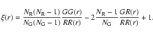
Here we adopt the Landy-Szalay estimator,
that expresses ![]() as
as
 |
(2) |
Observed distortions in galaxy surveys can be separated into two main
contributions: on small scales, the distortion is dominated by random
internal velocities in groups and clusters, causing a stretching of
![]() along the
along the ![]() direction (the so-called "fingers of
God'' effect). On large scales, on the other hand,
direction (the so-called "fingers of
God'' effect). On large scales, on the other hand,
![]() contours tend to be flatter, due to coherent infall of galaxies onto
large-scale overdensities, known as the "Kaiser effect''
(Kaiser 1987). The latter is a weak effect and needs very large
samples to be seen with sufficient accuracy, as shown by the 2dF survey
(Hawkins et al. 2003).
contours tend to be flatter, due to coherent infall of galaxies onto
large-scale overdensities, known as the "Kaiser effect''
(Kaiser 1987). The latter is a weak effect and needs very large
samples to be seen with sufficient accuracy, as shown by the 2dF survey
(Hawkins et al. 2003).
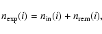
We can recover the real-space correlation function ![]() by
projecting
by
projecting
![]() along the line of sight, onto the
along the line of sight, onto the ![]() axis. In this way we integrate out the dilution produced by the
redshift-space distortion field and obtain a quantity,
axis. In this way we integrate out the dilution produced by the
redshift-space distortion field and obtain a quantity,
![]() ,
which is independent
of the redshift-space distortions:
,
which is independent
of the redshift-space distortions:
Ideally, if the studied data set consisted of a large enough number
of statistically independent pairs, such that the central limit theorem
applies, then the distribution of estimates of ![]() in an ensemble of
similar samples should be Gaussian. The
in an ensemble of
similar samples should be Gaussian. The ![]() uncertainty - the
"cosmic error''- in
uncertainty - the
"cosmic error''- in ![]() would then be the square root of its
variance
would then be the square root of its
variance
![]() (Peebles 1973). However, the
theoretical expression for
(Peebles 1973). However, the
theoretical expression for
![]() depends on the poorly
known and difficult to measure four-point correlation function.
Moreover, since the measured
depends on the poorly
known and difficult to measure four-point correlation function.
Moreover, since the measured ![]() is not exactly coincident with the
theoretical
is not exactly coincident with the
theoretical ![]() ,
we expect its uncertainty to be
also somewhat different from the value provided by the
theory. This effect is known as a cosmic bias.
,
we expect its uncertainty to be
also somewhat different from the value provided by the
theory. This effect is known as a cosmic bias.
A few different ways of estimating errors on two-point correlation functions have been used in the literature (for a wider discussion, see e.g. Hamilton 1993; Fisher et al. 1994; Bernardeau et al. 2002). The case closest to the ideal situation is when the survey is large enough that it can be split into a number of sub-samples. Correlations are then estimated independently for each of these, and error bars for the parent sample computed as the rms values. This has been for example the case of the angular correlation function from the APM survey (e.g. Maddox et al. 1990). However, the number of sub-samples cannot be large, otherwise the explored scales will be significantly reduced with respect to the parent survey. The consequence is that the variance is typically overestimated and these represent usually upper limits to the true errors.
Simple Poissonian errors (e.g. proportional to the square root of the
total number of galaxy pairs in each bin) underestimate the error bars
substantially. Statistical corrections were proposed
(Kaiser 1986) by multiplying Poissonian errors by a factor
![]() ,
with n being the number density of objects and
,
with n being the number density of objects and
![]() ,
where we assume that the actual correlation
function vanishes for
,
where we assume that the actual correlation
function vanishes for
![]() .
However, this method also tends to
give relatively small errors (Fisher et al. 1994).
.
However, this method also tends to
give relatively small errors (Fisher et al. 1994).
Over the last twenty years a widely used method has been the
so-called "bootstrap resampling''
(Barrow et al. 1984). It is based on the idea of "perturbing'' the data
set, by randomly creating a large number of comparable "pseudo
data-sets'', which differ only slightly from the original sample.
If this contains N objects, then each bootstrap sample is created
selecting N of these, but allowing for multiple selections of the
same object. This means that some objects will not be included in one
given pseudo data-set, while others will be counted twice or three times.
This is a good test of the robustness of measured correlations,
especially on large scales where having a large number of pairs does
not always mean a robust measurement: consider for example the case of
a single isolated galaxy at a separation of ![]() from a cluster
containing 1000 galaxies.
from a cluster
containing 1000 galaxies.
![]() will contain a large number
of pairs, however only one will be independent. On the other hand,
bootstrap errors often tend to over-estimate the theoretical variance
will contain a large number
of pairs, however only one will be independent. On the other hand,
bootstrap errors often tend to over-estimate the theoretical variance
![]() .
In general, however, despite debates on their
theoretical justification, they have represented a practical way to
obtain error bars in correlation analysis which are not far from the
true ones.
.
In general, however, despite debates on their
theoretical justification, they have represented a practical way to
obtain error bars in correlation analysis which are not far from the
true ones.
The use of bootstraping became less and less popular in recent years, with the advent of large N-body simulations, reproducing the matter distribution over significant volumes of the Universe. Coupled to physically sound definitions of "galaxies'', these allowed the construction of sets of independent mock surveys, from which ensemble errors could be computed from the scatter in the different catalogs. This is the same technique used to construct our VVDS mock surveys. Clearly, a good match is necessary between the volume and resolution of the simulation, on one side, and the depth and size of the survey on the other. Furthermore, the power spectrum of the simulation must provide a realistic description of long waves, so to properly include cosmic variance. Progress both in our knowledge of structure on the largest scales and in the size and resolution of N-body simulations has improved on early applications of this technique (Fisher et al. 1994). For this reason, since the GalICS simulations are available, we could use this as our main method for error estimation.
However, as we detail below, the covariance matrix reconstructed from the simulations cannot be applied in a straightforward way to the observed data. Indeed, our fitting technique, discussed below, handles the covariance matrix to properly account for bin-to-bin correlations when fitting correlation functions: when the covariance matrix extracted from the set of 50 mock VVDS surveys is used (after proper normalization of the average values), the fit is often unstable. In other words, the covariance matrix produced by the ensemble of mock surveys, although providing sufficiently realistic diagonal elements, has off-diagonal non-zero values which differ from those pertaining to the data sample (which of course are unknown). For this reason, we modified our strategy and resort to the bootstrap technique to estimate the bin-to-bin covariance. This means that our error bars on the estimated correlation functions are obtained via the more reliable scatter between the mock surveys, but a bootstrap is used to estimate the off-diagonal terms of the covariance matrix.
Let us consider a given redshift slice
[z1 - z2]. Within this
same interval, we estimate the correlation function
![]() from: 1) 50 mock VVDS surveys; 2) the real VVDS data;
3)
from: 1) 50 mock VVDS surveys; 2) the real VVDS data;
3)
![]() (typically 100) bootstrap resamplings of the VVDS data.
We then compute, for each of these estimates,
(typically 100) bootstrap resamplings of the VVDS data.
We then compute, for each of these estimates,
![]() ,
projecting
,
projecting
![]() along the line of sight (Eq. (3)), with an
upper integration limit
along the line of sight (Eq. (3)), with an
upper integration limit
![]() ,
chosen in practice so that it is
large enough to produce a stable estimate of
,
chosen in practice so that it is
large enough to produce a stable estimate of
![]() .
Similarly to other authors (see e.g. Guzzo et al. 1997), we find
.
Similarly to other authors (see e.g. Guzzo et al. 1997), we find
![]() quite insensitive to the choice of
quite insensitive to the choice of
![]() in the range
of
in the range
of
![]() for
for
![]() .
Too small a value for this limit would miss small-scale power, while
too large a value has the effect of adding noise into
.
Too small a value for this limit would miss small-scale power, while
too large a value has the effect of adding noise into ![]() .
After a
set of experiments we have chosen
.
After a
set of experiments we have chosen
![]() .
.
In the following, we call
![]() the value of
the value of ![]() ,
computed
at
,
computed
at
![]() in the cone k, where
in the cone k, where
![]() if we
consider the GalICS data or
if we
consider the GalICS data or
![]() if we
consider the bootstrap data.
If not otherwise mentioned,
if we
consider the bootstrap data.
If not otherwise mentioned,
![]() is used.
is used.
Whether we
consider the mock or bootstrap samples,
we can always compute the associated covariance matrix, ![]() ,
between the
values of
,
between the
values of ![]() in ith and kth bins:
in ith and kth bins:
| (6) |
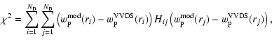 |
(7) |
In principle, the complete process could be done using only our set of
50 mock VVDS surveys. In practice, as explained above,
the bin-to-bin covariance obtained from the GalICS mock samples
does not provide a statistically stable matrix to be used
with the generalized ![]() method. Therefore, we most appropriately used
the covariance
matrix obtained from the
method. Therefore, we most appropriately used
the covariance
matrix obtained from the
![]() bootstrap resamplings
of the galaxy data set.
bootstrap resamplings
of the galaxy data set.
This provides the best solution for
![]() that minimizes
the error contour
that minimizes
the error contour
![]() .
At the same time, however, we use 50 mock
surveys to obtain the most realistic error contours
.
At the same time, however, we use 50 mock
surveys to obtain the most realistic error contours
![]() on our estimated
on our estimated
![]() ,
as these - unlike bootstrap errors - include cosmic
variance.
,
as these - unlike bootstrap errors - include cosmic
variance.
The final error contours, therefore, are obtained fitting the mean of the
50 ![]() mock VVDS surveys, using a covariance matrix computed from the same
50
mock VVDS surveys, using a covariance matrix computed from the same
50 ![]() .
This process provides a solution for
.
This process provides a solution for
![]() associated with the
error contours
associated with the
error contours
![]() .
We then re-center these contours
around
.
We then re-center these contours
around
![]() with the renormalization
with the renormalization
![]() and
and
![]() .
.
To take into account the different N(z) of GalICS and VVDS, we multiply
the error contour
![]() computed for each redshift slice by
a factor
computed for each redshift slice by
a factor
![]() ,
where
,
where
![]() is the number of VVDS galaxies
and
is the number of VVDS galaxies
and
![]() is the number of GalICS galaxies in this redshift slice.
is the number of GalICS galaxies in this redshift slice.
The error bars computed as above for each
![]() value correspond
to the rms of the 50
value correspond
to the rms of the 50
![]() ,
normalized to the data.
,
normalized to the data.
We now quantitatively establish the impact of the VVDS selection effects on the measured correlations and the accuracy of our correcting scheme, using the GalICS mock samples.
As we have seen in the previous section, the biases and selection
effects due to the observing strategy and instrumental limitations
affect the properties of the angular distribution of
objects, with respect to a random sub-sampling of
galaxy clustering process. It is therefore the angular correlation
function
![]() that will primarily reflect these biases.
Clearly, there is no specific scientific reason to measure the
angular correlation function from the spectroscopic sample, as this
can be done more easily and with much greater confidence using the
full VVDS photometric catalog (McCracken et al. 2003).
that will primarily reflect these biases.
Clearly, there is no specific scientific reason to measure the
angular correlation function from the spectroscopic sample, as this
can be done more easily and with much greater confidence using the
full VVDS photometric catalog (McCracken et al. 2003).
![]() allows us to illustrate the level
of distortions introduced by our angular
selection function.
allows us to illustrate the level
of distortions introduced by our angular
selection function.
To this end,
Fig. 8 shows the angular correlation function computed
from one mock VVDS redshift survey without
correcting for these effects (i.e. using a random sample which simply
follows the geometrical borders of the galaxy sample, as one would do
for a homogeneous angular selection), compared to that of the original
mock catalog.
![\begin{figure}
\par\includegraphics[width=7.3cm,clip]{1964fi09.ps} \end{figure}](/articles/aa/full/2005/33/aa1964-04/img100.gif) |
Figure 8:
Impact of
the observational process on the estimate of the angular two-point
correlation function
|
| Open with DEXTER | |
The biases discussed so far involve introducing two types of corrections which we discuss in detail in this section.
1) Global correction. To account for the effects of uneven boundaries and varying sampling rate we construct a random catalog, which consists of the same number of separately created pointings as the galaxy sample, thus reproducing the global "exposure map'' (i.e. number of multiple passes over a given point of the sky) and the corresponding large-scale surface density variations of the galaxy redshift sample. The holes and excised regions in the photometric sample are similarly taken into account by applying the same binary mask to the random sample. These first-order corrections account already for most of the observational biases. When taken into account, they reduce most of the negative effects of the observing strategy on the correlation functions, in particular the global overestimation of correlation functions (see Figs. 9-11).
2) Small scale correction.
What remains to be corrected is
the slight bias introduced by the
slit-positioning software and the mechanical limitations (slit size,
closeness of slits and so forth). We have seen that the
SSPOC selection is
not an entirely random sampling of the actual
angular distribution of objects, but rather a more homogeneous sub-set,
preferentially concentrated along specific rows. This selection
affects primarily the small-scale values of the correlation function,
corresponding to the typical slit size: with only one spectroscopic
pass, pairs of galaxies with separation smaller than the slit size
will always have only one galaxy observed, and thus their contribution
to ![]() will be lost. With repeated passes this problem is
alleviated, as the software chooses each time different objects (except for a
small number of objects observed twice for error checking purposes).
Using the full 2D information available from the parent photometric
catalog (that tells us how many galaxies on the sky have been missed in
the spectroscopic sample), we developed a weighting scheme that weighs
each targeted galaxy proportionally to its "representativity'' in
terms of local angular pair density.
will be lost. With repeated passes this problem is
alleviated, as the software chooses each time different objects (except for a
small number of objects observed twice for error checking purposes).
Using the full 2D information available from the parent photometric
catalog (that tells us how many galaxies on the sky have been missed in
the spectroscopic sample), we developed a weighting scheme that weighs
each targeted galaxy proportionally to its "representativity'' in
terms of local angular pair density.
![\begin{figure}
\par\includegraphics[width=7.6cm,clip]{1964fi10.ps}\hspace*{5mm}
\includegraphics[width=7.6cm,clip]{1964fi11.ps} \end{figure}](/articles/aa/full/2005/33/aa1964-04/img101.gif) |
Figure 9:
Redshift-space two-point correlation function |
| Open with DEXTER | |
![\begin{figure}
\par\includegraphics[width=7.6cm,clip]{1964fi12.ps}\hspace*{5mm}
\includegraphics[width=7.6cm,clip]{1964fi13.ps} \end{figure}](/articles/aa/full/2005/33/aa1964-04/img102.gif) |
Figure 10:
Same as Fig. 9, but for the
|
| Open with DEXTER | |
![\begin{figure}
\par\includegraphics[width=7.6cm,clip]{1964fi14.ps}\hspace*{5mm}
\includegraphics[width=7.6cm,clip]{1964fi15.ps} \end{figure}](/articles/aa/full/2005/33/aa1964-04/img103.gif) |
Figure 11:
Same as Figs. 9 and 10, but for the projected function
|
| Open with DEXTER | |
Let us therefore consider a circular region of radius ![]() around a galaxy i located within a specific redshift slice k, and
define inside
around a galaxy i located within a specific redshift slice k, and
define inside ![]() the following quantities:
the following quantities:
![]() - the number of galaxies in the parent photometric catalog;
- the number of galaxies in the parent photometric catalog;
nz(i) - the number of galaxies with measured redshift;
![]() - the subset of these belonging to the same redshift
slice as the central galaxy;
- the subset of these belonging to the same redshift
slice as the central galaxy;
![]() - the number of
galaxies expected to belong to the same redshift slice, which can be
written as
- the number of
galaxies expected to belong to the same redshift slice, which can be
written as
 |
(8) |
![\begin{displaymath}n_{\rm rem}(i) = [n_{\rm gal}(i) - n_z(i)]*P_{\rm slice} ,
\end{displaymath}](/articles/aa/full/2005/33/aa1964-04/img110.gif) |
(9) |
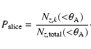 |
(10) |
The construction of the actual weight to recover the loss of
small-scale pairs produced essentially by the proximity bias is not
unequivocal. After several experiments with weighting by local
densities (of expected vs. observed spectra), we obtained the best
results weighting by pairs.
The two-point correlation function being a pair-weighted statistic,
we constructed our weight w(i) for a given galaxy ifrom the ratio of the expected to the measured number of pairs within
![]() .
Specifically, if one wants the local angular pair density
to be conserved, each pair should be counted as:
.
Specifically, if one wants the local angular pair density
to be conserved, each pair should be counted as:
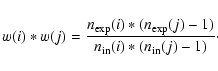 |
(11) |
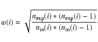 |
(12) |
The following sections will present the results of extensive tests of this correction scheme, based on the GalICS mock VVDS surveys.
We have applied the manipulations presented in the previous section to our
mock VVDS 02h
surveys and compared the results to those obtained from the
whole 1
![]() mock
fields.
The results are shown in Figs. 9-11 for the same mock sample
used for measuring
mock
fields.
The results are shown in Figs. 9-11 for the same mock sample
used for measuring
![]() (Fig. 8), split into 4
redshift bins. In each of these figures, comparison of the the
four left to the four right panels demonstrates the
effect of the overall correction.
In general,
in redshift space the effect of the observational biases
is much less severe, being diluted by the unaffected clustering measured along
the line of sight. Still, we see how a proper estimate
does require a correction.
(Fig. 8), split into 4
redshift bins. In each of these figures, comparison of the the
four left to the four right panels demonstrates the
effect of the overall correction.
In general,
in redshift space the effect of the observational biases
is much less severe, being diluted by the unaffected clustering measured along
the line of sight. Still, we see how a proper estimate
does require a correction.
Looking at ![]() (Fig. 9), we see that the correction introduced by our scheme is
in general very good.
The full bi-dimensional correlation function
(Fig. 9), we see that the correction introduced by our scheme is
in general very good.
The full bi-dimensional correlation function
![]() (Fig. 10) shows the effect in more detail, indicating
also that the impact of the angular bias on spatial correlations
depends on redshift. This is to be expected, given that a fake
inhomogeneity at a given angular scale affects larger spatial scales
at larger redshifts.
However, as seen from the four right panels
the bulk of the problem is corrected by our technique.
(Fig. 10) shows the effect in more detail, indicating
also that the impact of the angular bias on spatial correlations
depends on redshift. This is to be expected, given that a fake
inhomogeneity at a given angular scale affects larger spatial scales
at larger redshifts.
However, as seen from the four right panels
the bulk of the problem is corrected by our technique.
Finally, the
corresponding projected function,
![]() ,
which is the one that will be fitted to estimate the real-space correlation
length and slope,
(Le Fèvre et al. 2005), does not show
any significant systematic effect, nor scale-dependent bias (see also
Sect. 6.4, below), if one excludes a residual effect
in the highest-redshift bin (which may be specific of the mock sample
used).
,
which is the one that will be fitted to estimate the real-space correlation
length and slope,
(Le Fèvre et al. 2005), does not show
any significant systematic effect, nor scale-dependent bias (see also
Sect. 6.4, below), if one excludes a residual effect
in the highest-redshift bin (which may be specific of the mock sample
used).
Let us now evaluate more quantitatively how well the weighting
scheme
is able to recover the correct values of the two
parameters of ![]()
![]() ,
r0 and
,
r0 and ![]() .
Figure 12 plots the projected correlation function
.
Figure 12 plots the projected correlation function
![]() ,
computed for one of the VVDS mock cones, together with
the measured best fit values of r0 and
,
computed for one of the VVDS mock cones, together with
the measured best fit values of r0 and ![]() .
The error contours are estimated from the variance of the 50 mock surveys as
described previously and their size
depends mainly on the number of galaxies within each bin.
Figure 13 shows that the evolution of clustering we "observe'' in
this specific simulated VVDS cone agrees quite well with its parent
sample.
.
The error contours are estimated from the variance of the 50 mock surveys as
described previously and their size
depends mainly on the number of galaxies within each bin.
Figure 13 shows that the evolution of clustering we "observe'' in
this specific simulated VVDS cone agrees quite well with its parent
sample.
Of course, due to cosmic variance, the values of r0 and ![]() differ between different simulated cones. Figure 14 shows
the spread of these parameters among all the 50 mock VVDS surveys
and their parent catalogs, for a representative redshift bin (
z=[0.5-0.7]). This
behavior is similarly seen in the other redshift bins, indicating an
increased spread in the parameter estimates in the "observed''
catalogs, an effect easily explained in terms of the smaller number of objects.
Figures 12 and 14 also indicate that
at the end of our correction process
any possible systematic effect is reduced to less than 5%, a
value
always significantly smaller than the
uncertainty due to cosmic variance which is
of the order of 15-20%.
differ between different simulated cones. Figure 14 shows
the spread of these parameters among all the 50 mock VVDS surveys
and their parent catalogs, for a representative redshift bin (
z=[0.5-0.7]). This
behavior is similarly seen in the other redshift bins, indicating an
increased spread in the parameter estimates in the "observed''
catalogs, an effect easily explained in terms of the smaller number of objects.
Figures 12 and 14 also indicate that
at the end of our correction process
any possible systematic effect is reduced to less than 5%, a
value
always significantly smaller than the
uncertainty due to cosmic variance which is
of the order of 15-20%.
![\begin{figure}
\includegraphics[width=8.2cm,clip]{1964fi16.ps} \end{figure}](/articles/aa/full/2005/33/aa1964-04/img127.gif) |
Figure 12:
Evolution of the projected function
|
| Open with DEXTER | |
![\begin{figure}
\par\includegraphics[width=7.6cm,clip]{1964fi17.ps} \end{figure}](/articles/aa/full/2005/33/aa1964-04/img128.gif) |
Figure 13: Evolution of r0 in a VVDS mock survey (filled circles), compared to that of its parent catalog (open circles). Error bars are as explained in the text. The "true'' and "measured'' values of r0 are very consistent within the error bars, providing an internal proof of the quality of our correction scheme. |
| Open with DEXTER | |
![\begin{figure}
\par\includegraphics[width=7.7cm,clip]{1964fi18.ps} \end{figure}](/articles/aa/full/2005/33/aa1964-04/img129.gif) |
Figure 14:
Histograms of the measurements of
r0 and |
| Open with DEXTER | |
In this section we want to
discuss from a more general perspective (i.e.
not limited to the current status and lay-out of the 02h field) how
the accuracy of correlation measurements can
depend on
the number of multiple spectroscopic pointings ("passes'') that are
dedicated to a specific area. In other words: are multiple passes
increasing - as expected - the accuracy of correlation function
measurements, not only thanks to the increased statistics, but also
because of the improved sampling of the clustering process? And how is
our correcting scheme performing when handling a very sparse (one
pass) or a more densely sampled area? This is clearly an
interesting question for the future development of the VVDS,
or other surveys, as these
tests can indicate what strategy could be more efficient.
One would like to estimate the fraction of galaxies
necessary
to recover the correlation signal
to a certain level of accuracy. This,
translated to the VVDS, implies determining how many spectroscopic "passes''
with VIMOS are necessary. Note that the answer is
not trivial, since multiple pointings over the same area are usually
dithered (i.e. shifted by an amount at least larger than the central
"cross'', i.e. 2![]() ), and thus a larger number of passes over
the same area, while improving the sampling, introduces also a more
complex mean density pattern, as explained in Sect. 2.1.
), and thus a larger number of passes over
the same area, while improving the sampling, introduces also a more
complex mean density pattern, as explained in Sect. 2.1.
Tests have been performed creating a grid of six pointings, spaced
with the same step as the real VVDS ones in the VVDS-10h field. The second
pass was then arranged over a grid shifted by
![]() in right ascension and declination. The pointings of both passes
have then been "observed'' once again with a different selection of objects
for spectroscopy. At the end (maximum coverage), this
resulted in an area of 0.3624 square degrees, mostly uniformly covered
but with small patches of sky that were observed either three,
two or one times or remained unobserved.
The results for
in right ascension and declination. The pointings of both passes
have then been "observed'' once again with a different selection of objects
for spectroscopy. At the end (maximum coverage), this
resulted in an area of 0.3624 square degrees, mostly uniformly covered
but with small patches of sky that were observed either three,
two or one times or remained unobserved.
The results for
![]() and
and ![]() are shown in Figs. 15 and 16, respectively.
are shown in Figs. 15 and 16, respectively.
![\begin{figure}
\par\includegraphics[width=7.7cm,clip]{1964fi19.ps} \end{figure}](/articles/aa/full/2005/33/aa1964-04/img132.gif) |
Figure 15:
Measured
|
| Open with DEXTER | |
The
projected correlation function ![]() is fairly well
recovered almost independently of the sampling density.
For a single pass, power is
not recovered properly at
scales below 0.6 h-1 Mpc, since there is in practice no pair (even biased) to be
"corrected'' in a proper statistical way by our scheme.
is fairly well
recovered almost independently of the sampling density.
For a single pass, power is
not recovered properly at
scales below 0.6 h-1 Mpc, since there is in practice no pair (even biased) to be
"corrected'' in a proper statistical way by our scheme.
The case of ![]() (Fig. 16) shows even more clearly the
difficulty of recovering very small scale pairs with only one pass:
in this case, there is an intrinsic low-scale limitation (complete
lack of pairs), which cannot be fully overcome by the correcting
scheme. The figure shows, for example, that while a linear bin
between 0 and 1
(Fig. 16) shows even more clearly the
difficulty of recovering very small scale pairs with only one pass:
in this case, there is an intrinsic low-scale limitation (complete
lack of pairs), which cannot be fully overcome by the correcting
scheme. The figure shows, for example, that while a linear bin
between 0 and 1
![]() is already sufficient to recover the
correct clustering amplitude even with one pass, smaller
logarithmic bins below 1
is already sufficient to recover the
correct clustering amplitude even with one pass, smaller
logarithmic bins below 1
![]() are inadequate and suffer from the lack
of measured pairs.
are inadequate and suffer from the lack
of measured pairs.
![\begin{figure}
\par\includegraphics[width=7.5cm,clip]{1964fi20.ps} \end{figure}](/articles/aa/full/2005/33/aa1964-04/img134.gif) |
Figure 16:
Measurements of |
| Open with DEXTER | |
We conclude that even in the fields that were observed only with one
spectroscopic observation, sampling about 15% of the photometric
targets down to IAB=24,
the two-point correlation function can be measured quite well
for separations
![]() Mpc.
The results confirm, however, that observing fields four times,
sampling about 40% of the population
as in the deep part of the VVDS, provides the possibility of
more precise measurements on
scales
down to 0.1 h-1 Mpc.
Mpc.
The results confirm, however, that observing fields four times,
sampling about 40% of the population
as in the deep part of the VVDS, provides the possibility of
more precise measurements on
scales
down to 0.1 h-1 Mpc.
One of the key goals of the VVDS survey is to measure the evolution of
the galaxy clustering from the present epoch up to ![]() and
larger. To study in detail the error budget of
and
larger. To study in detail the error budget of ![]() measurements in
the VVDS survey, we have generated a set of mock catalogs using the
GalICS model of semi-analytic galaxy formation. The geometry of the
VVDS survey on the sky is complex due to the observing strategy. The
resulting selection function substantially affects the angular correlation
properties of the clustering of the observed galaxies. We demonstrate
that the correlation observed in redshift space is much less
affected and that the
bias introduced by the observing strategy can be largely removed using
the correcting scheme we propose in this paper.
measurements in
the VVDS survey, we have generated a set of mock catalogs using the
GalICS model of semi-analytic galaxy formation. The geometry of the
VVDS survey on the sky is complex due to the observing strategy. The
resulting selection function substantially affects the angular correlation
properties of the clustering of the observed galaxies. We demonstrate
that the correlation observed in redshift space is much less
affected and that the
bias introduced by the observing strategy can be largely removed using
the correcting scheme we propose in this paper.
We conclude that, for the first epoch VVDS data, we can expect
to measure ![]() and
and
![]() to better than 10% on scales
to better than 10% on scales
![]() h-1 Mpc, and better than 30% below 1 h-1 Mpc.
Results obtained from the
GalICS simulations indicate that the two-point correlation functions
computed from the First Epoch VVDS should suffer only from a modest cosmic
variance of
h-1 Mpc, and better than 30% below 1 h-1 Mpc.
Results obtained from the
GalICS simulations indicate that the two-point correlation functions
computed from the First Epoch VVDS should suffer only from a modest cosmic
variance of
![]() %. These results suggest
that after the final selection of objects for spectroscopy the variance
becomes twice as large as the variance of the underlying parent galaxy
field in the same area. We expect,
in each redshift slice
%. These results suggest
that after the final selection of objects for spectroscopy the variance
becomes twice as large as the variance of the underlying parent galaxy
field in the same area. We expect,
in each redshift slice
![]() in the
redshift range
z=[0.2,2.1], to measure r0 and
in the
redshift range
z=[0.2,2.1], to measure r0 and ![]() with an accuracy better than
with an accuracy better than ![]() .
We show
that any residual systematic effect in the measurements of r0and
.
We show
that any residual systematic effect in the measurements of r0and ![]() is
below
5%, i.e. a value
much smaller than the cosmic errors.
is
below
5%, i.e. a value
much smaller than the cosmic errors.
The actual measured clustering properties of galaxies in the VVDS survey, using the framework outlined in this paper, are presented in Le Fèvre et al. (2005b) and in forthcoming papers.
Acknowledgements
We thank the GalICS group for access to their simulations, S. Colombi for providing a first set of mock n-body samples early in the development of this work and for useful discussions. This research has been developed within the framework of the VVDS consortium and has been partially supported by the CNRS-INSU and its Programme National de Cosmologie (France), and by Italian Research Ministry (MIUR) grants COFIN2000 (MM02037133) and COFIN2003 (No. 2003020150).
![\begin{displaymath}w_{\rm p}(r_{\rm p}) \equiv 2 \int_0^\infty \xi(r_{\rm p},\pi...
...infty
\xi_\circ\left[(r_{\rm p}^2+y^2)^{1/2}\right] {\rm d}y.
\end{displaymath}](/articles/aa/full/2005/33/aa1964-04/img53.gif)