A&A 439, 443-459 (2005)
DOI: 10.1051/0004-6361:20041511
J. Pétri![]()
Astronomical Institute, University of Utrecht, PO Box 80000, 3508 TA Utrecht, The Netherlands
Received 22 June 2004 / Accepted 12 April 2005
Abstract
Quasi-periodic oscillations (QPOs) have been observed in accretion
disks around neutron star, black hole, and white dwarf binaries with
frequencies ranging from a few 0.1 Hz up to 1300 Hz. Recently, a
correlation between their low- and high-frequency components was
discovered and fitted with a single law, irrespective of the nature
of the compact object. That such a relation holds over 6 orders of
magnitude strongly supports the idea that the physical mechanism
responsible for these oscillations should be the same in all binary
systems.
We propose a new model for these QPOs based on forced oscillations
induced in the accretion disk due to the stellar magnetic field.
First, it is shown that a magnetized accretion disk evolving in a
rotating nonaxisymmetric magnetic field anchored to a neutron star
will be subject to three kinds of resonances: a corotation
resonance, a Lindblad resonance due to a driving force, and a
parametric resonance due to the time varying epicyclic frequencies.
The asymmetric part of the field is assumed to contain only one
azimuthal mode ![]() .
We focus on the m=1 disturbance, which is
well studied for an inclined dipolar rotator; but our results are
general and easily extend to m>1. However, the radial location of
the resonances will be affected by this number m. For instance,
with an m=1 asymmetric structure, the resonances reach regions
very close to the innermost stable circular orbit (ISCO) and can
account for observations of kHz-QPOs at frequencies as high
as 1200-1300 Hz. If we replace the dipolar by a higher order
multipolar component, the resonance location is shifted to larger
radius, implying lower QPO frequencies. To compare the MHD situation
with the hydrodynamical case, we also consider an m=2 component in
the magnetic perturbation in order to prove that, at least in the
linear regime, the conclusions in both cases are the same. In the
second part of the paper, we focus on the linear response of a thin
accretion disk, developing the density perturbation as the sum of
free wave solutions and non-wavelike disturbances. In the last part,
we show results of 2D numerical simulations of a simplified version
of the accretion disk consisting of a column of plasma threaded by a
vertical magnetic field. These simulations are performed for the
Newtonian gravitational potential, as well as for a pseudo-general
relativistic potential, which enables us to explore the behavior of
the resonances around both rotating neutron stars and black holes.
We found that the density perturbations are only significant in the
region located close to the inner edge of the disk near the ISCO
where the magnetic perturbation is maximal. They induce
fluctuations in the density which persist over the whole time of the
simulations and are closely related to the spin of the magnetic
perturbation. It is argued that the nearly periodic motion induced
in the disk will produce high quality factor QPOs.
.
We focus on the m=1 disturbance, which is
well studied for an inclined dipolar rotator; but our results are
general and easily extend to m>1. However, the radial location of
the resonances will be affected by this number m. For instance,
with an m=1 asymmetric structure, the resonances reach regions
very close to the innermost stable circular orbit (ISCO) and can
account for observations of kHz-QPOs at frequencies as high
as 1200-1300 Hz. If we replace the dipolar by a higher order
multipolar component, the resonance location is shifted to larger
radius, implying lower QPO frequencies. To compare the MHD situation
with the hydrodynamical case, we also consider an m=2 component in
the magnetic perturbation in order to prove that, at least in the
linear regime, the conclusions in both cases are the same. In the
second part of the paper, we focus on the linear response of a thin
accretion disk, developing the density perturbation as the sum of
free wave solutions and non-wavelike disturbances. In the last part,
we show results of 2D numerical simulations of a simplified version
of the accretion disk consisting of a column of plasma threaded by a
vertical magnetic field. These simulations are performed for the
Newtonian gravitational potential, as well as for a pseudo-general
relativistic potential, which enables us to explore the behavior of
the resonances around both rotating neutron stars and black holes.
We found that the density perturbations are only significant in the
region located close to the inner edge of the disk near the ISCO
where the magnetic perturbation is maximal. They induce
fluctuations in the density which persist over the whole time of the
simulations and are closely related to the spin of the magnetic
perturbation. It is argued that the nearly periodic motion induced
in the disk will produce high quality factor QPOs.
Key words: accretion, accretion disks - magnetohydrodynamics (MHD) - instabilities - methods: analytical - methods: numerical - stars: neutron
To date, more than 20 accreting neutron stars in Low Mass X-Ray Binaries (LMXBs) are known to exhibit rapid variability in their X-ray fluxes. These high frequency quasi-periodic oscillations (QPOs) show very strong similarities in their shape, as well as in their amplitude, and span frequencies from 300 Hz to about 1300 Hz (see van der Klis 2000, for a review).
The comparison between high frequency QPOs (HFQPOs) in black holes and neutron stars shows a scaling proportional to 1/M*, where M* is the mass of the compact object, suggesting that these oscillations are due to the orbital motion in the accretion disk near the innermost stable circular orbit (ISCO) (McClintock & Remillard 2003). Moreover, the QPO frequencies depend on the spectral state of the source and are correlated with the accretion rate. QPOs are observed in the tail of the power law spectrum indicating that they are not due to thermal emission but probably related to Comptonization of soft photons. The saturation of the spectral index was explained by Titarchuk & Fiorito (2004) in the context of coronal heating and phase transition.
Therefore, any QPO model must take not only oscillations in the accretion disk into account but also the way photons propagate to the observer, including photon scattering and general relativistic effects such as beaming, Doppler shift, and aberration. This was investigated by Schnittman & Bertschinger (2004), who used exact integration of the geodesic motion of hot spots in the Kerr spacetime and looked at the harmonic content of the signal received by an observer in the asymptotically flat spacetime.
In black hole binaries, the HFQPOs appear in pairs, as in the neutron star system, but their frequency remains uncorrelated to the accretion rate. They act as a voiceprint at a ratio 3:2 that favors a resonance mechanism. For example a parametric resonance between vertical and horizontal epicyclic frequencies was suggested by Kluzniak et al. (2004). Another mechanism proposed by Lee et al. (2004) is resonance due to an external driven force.
The physics of accretion onto a magnetized neutron star has been described by Ghosh & Lamb (1978, 1979a,b). In this picture close to the star's surface, the magnetic field channels matter to the polar caps and exerts a torque on it, which accelerates or decelerates the neutron star depending on the angular momentum exchange rate. This is the standard model of magnetized accretion onto a neutron star. However, in order to explain pulsating X-ray sources, Anzer & Börner (1980) propose an alternative view in which the magnetic moment of the neutron star and the accretion disk rotation axis are perpendicular. They also studied the influence of the Kelvin-Helmholtz instability on such a configuration (Anzer & Börner 1983).
When the magnetic moment is misaligned with respect to the spin axis of the star, Vietri & Stella (1998) show that some inhomogeneities, treated as diamagnetic blobs, could be lifted off the disk and suffer the Lense-Thirring precession.
Lai (1999) has identified a magnetically driven warping and precession instability that occurs in the inner region of an accretion disk. This occurs by interaction between the surface current density in the disk with the stellar magnetic field and produces motions at frequencies much lower than the orbital one. It can, therefore, account for the low frequency QPOs (LFQPOs), as does the usual Lense-Thirring precession (Stella & Vietri 1998). Magnetic precession, combined with the relativistic dragging effect, was applied to weakly magnetized neutron stars to explain these LFQPOS in LMXBs, (Shirakawa & Lai 2002a). The study of the global magnetic warping/precession process for strongly magnetized neutron stars can also explain the millihertz QPOs in some systems, see for example Shirakawa & Lai (2002b). The Rayleigh-Taylor instability associated with Rossby waves and the rotational splitting gives another self-consistent description of the QPO phenomenon (Titarchuk 2003).
It was realized by Kato (2001a,b) that non-axisymmetric g-mode oscillations can be trapped in a thin relativistic disk. These are excited by the corotation resonance. The effect of non-linear coupling between oscillations in the disk and warp is examined by Kato (2004). However, his study does not include the rotation of the compact object.
Recent observations of accretion disks orbiting white dwarfs, neutron stars, or black holes have shown a strong correlation between the low and high frequency QPOs, LFQPOs and HFQPOs respectively, (Psaltis et al. 1999; Mauche 2002; Belloni et al 2002). This relation holds over more than 6 orders of magnitude and strongly supports the idea that the QPO phenomenon is a universal physical process independent of the nature of the compact object. Indeed, the presence or absence of a solid surface, a magnetic field, or an event horizon plays no relevant role in the production of X-ray variability (Wijnands 2001). This correlation has instead been explained in terms of the centrifugal barrier model of Titarchuk et al. (2002) where the LFQPOs are associated with magneto-acoustic waves, and the HFQPOs correspond to the Keplerian motion in the disk.
In this paper we propose a new resonance in the star-disk system arising from the response of the accretion disk to a non-axisymmetric rotating magnetic field. The paper is organized as follows. In Sect. 2, we describe the initial equilibrium state where the accretion disk is embedded in an axisymmetric magnetic field anchored to the neutron star. Furthermore, we assume that the magnetic moment is aligned with the rotation axis of the star. We then estimate the field perturbation induced by a small inclination of the magnetic moment. In Sect. 3, we look for the resonance conditions and elucidate the meaning of the resonances. For a thin and weakly magnetized accretion disk, assuming no warp and only motion in the orbital plane of the disk, we investigate the precise linear behavior of the disk which is presented in Sect. 3.2. In Sect. 5, we perform 2D numerical MHD simulations of the disk and show that some resonances persist on a long timescale with a narrow radial extension. This is done for Newtonian, as well as for pseudo-general relativistic gravitational potential describing the Kerr geometry in a Newtonian way adapted to a rotating neutron star. Conclusions are drawn in Sect. 6.
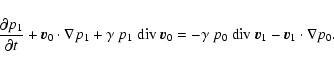
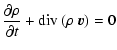
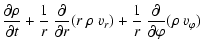
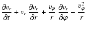
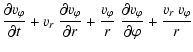
In the equilibrium state, the accretion disk evolves in a perfectly
spherically symmetric gravitational field and an axisymmetric dipolar
magnetic field, both due to the compact object. We assume that the
magnetic moment of the star and its rotational axis are aligned. The
disk is assumed to lie in the equatorial plane of the star so that it
experiences an axisymmetric stationary field. By adopting a
cylindrical coordinate system labeled by
![]() ,
we can
therefore describe all physical quantities with only a (r,z)dependence. Neglecting the matter inflow because in the thin disk
approximation
,
we can
therefore describe all physical quantities with only a (r,z)dependence. Neglecting the matter inflow because in the thin disk
approximation
![]() and because we only focus on
oscillations around a stationary state, the density
and because we only focus on
oscillations around a stationary state, the density ![]() ,
pressure p, current density
,
pressure p, current density ![]() ,
velocity
,
velocity ![]() ,
and
magnetic field
,
and
magnetic field ![]() at equilibrium are thus given by:
at equilibrium are thus given by:
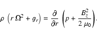
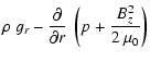
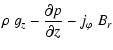
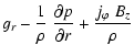
In the radial direction, the gravitational attraction from the compact
object ![]() is balanced by the centrifugal force, the Lorentz
force, and the pressure gradient, whereas in the vertical direction we
simply have hydromagnetic equilibrium:
is balanced by the centrifugal force, the Lorentz
force, and the pressure gradient, whereas in the vertical direction we
simply have hydromagnetic equilibrium:
In the case of an aligned rotator, ![]() ,
the magnetic field is
axisymmetric. Therefore, in the disk plane, there is only a vertical
component Bz. When the magnetic moment
,
the magnetic field is
axisymmetric. Therefore, in the disk plane, there is only a vertical
component Bz. When the magnetic moment ![]() is inclined by
an angle
is inclined by
an angle ![]() relative to rotation axis
relative to rotation axis
![]() ,
an
additional magnetic component dragged by the star's rotation arises.
This perturbation is responsible for the oscillation in the disk. We
derive its expression below. The magnetic moment can be developed into
a parallel (along
,
an
additional magnetic component dragged by the star's rotation arises.
This perturbation is responsible for the oscillation in the disk. We
derive its expression below. The magnetic moment can be developed into
a parallel (along ![]() )
and a perpendicular
(along
)
and a perpendicular
(along
![]() )
component such that
)
component such that
 |
(9) |
 |
(10) |
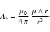
The angular rotation is assumed to be equal to
![]() .
The stellar dipolar magnetic field has the usual
expression derived from the vector potential
.
The stellar dipolar magnetic field has the usual
expression derived from the vector potential
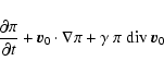
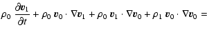
The distorted magnetic field described above will kick the disk out of
its equilibrium state. We study its linear response by treating the
asymmetric part of the magnetic field as a small perturbation of the
equilibrium state prescribed in Sect. 2. We start with
the ideal MHD equations of the accretion disk with adiabatic motion
given by:
We then perturb the equilibrium state from Sect. 2 by
introducing the Lagrangian displacement ![]() .
Expanding to
first order we get for the Eulerian perturbations of the
magnetohydrodynamical quantities attached to the disk:
.
Expanding to
first order we get for the Eulerian perturbations of the
magnetohydrodynamical quantities attached to the disk:
| (20) | |||
 |
(21) | ||
| (22) | |||
| (23) |
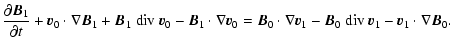
We make a clear distinction between the stellar magnetic
perturbation
![]() which is known at each time and given
by the rotating magnetic dipole
Eqs. (12)-(14) or any kind of
multipolar fluctuation associated with the star and those caused by
the current in the disk
which is known at each time and given
by the rotating magnetic dipole
Eqs. (12)-(14) or any kind of
multipolar fluctuation associated with the star and those caused by
the current in the disk
![]() in response to the former
perturbation.
in response to the former
perturbation.
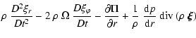
Expressing Eq. (24) in cylindrical coordinates for the
radial component leads to:
Finding an analytical stability criterion for this system is a
complicated or perhaps even an impossible task. Furthermore, we cannot
apply the classical expansion in plane wave solutions leading to an
eigenvalue problem. The presence of some coefficients varying
periodically in time, like
![]() ,
prevents such a
treatment. However, the problem can be cast in a more convenient form
if we decouple the oscillations in the orbital plane from those
perpendicular to it, as is done in the following subsection.
,
prevents such a
treatment. However, the problem can be cast in a more convenient form
if we decouple the oscillations in the orbital plane from those
perpendicular to it, as is done in the following subsection.
If we assume that there is no warping in the disk and neglect the
gradient and displacement in the vertical direction, we can perform a
detailed and accurate analysis of the motions in the disk. Indeed, by
setting ![]() and
and
![]() in Eqs. (25)
and (26), the linearized MHD equations become much more
tractable. Moreover, we first assume a simple geometric structure in
which the disk is replaced by a column of plasma threaded by a
vertical magnetic field and then allow only magnetic perturbation in
this direction. This situation seems far from the real system of an
oblique rotator; nevertheless, it gives a good first insight into the
oscillations and resonances arising there.
in Eqs. (25)
and (26), the linearized MHD equations become much more
tractable. Moreover, we first assume a simple geometric structure in
which the disk is replaced by a column of plasma threaded by a
vertical magnetic field and then allow only magnetic perturbation in
this direction. This situation seems far from the real system of an
oblique rotator; nevertheless, it gives a good first insight into the
oscillations and resonances arising there.
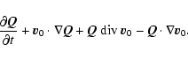
As a result, setting
![]() we find for the magnetic perturbation
we find for the magnetic perturbation
| Qr | = | 0 | (28) |
| = | 0 | (29) | |
| Qz | = | ![$\displaystyle - \frac{1}{r} ~ \left[ \frac{\partial}{\partial r}
\left( r ~ B_z...
...t) + \frac{\partial}{\partial \varphi}
\left( B_z ~ \xi_\varphi \right) \right]$](/articles/aa/full/2005/32/aa1511-04/img123.gif) |
(30) |
 |
(31) |
| (35) | |
| (36) |
| (38) | |||
 |
(39) |
 |
(41) |
When looking for free wave solutions to Eq. (40), we
can set
![]() .
Thus
.
Thus
| |
= | ![$\displaystyle - \left[ - \frac{3}{2} ~ \int_{r_{\rm L}}^r \sqrt{V(s)} ~ {\rm d}s \right]^{2/3}
{\rm for\;} r \le r_{\rm L}$](/articles/aa/full/2005/32/aa1511-04/img171.gif) |
(47) |
| = | ![$\displaystyle \left[ \frac{3}{2} ~ \int_{r_{\rm L}}^r \sqrt{-V(s)} ~ {\rm d}s \right]^{2/3}
{\rm for\;} r \ge r_{\rm L}.$](/articles/aa/full/2005/32/aa1511-04/img172.gif) |
(48) |
We emphasize that the qualitative results presented in this paper are independent of the nature of the spacetime, be it flat as in the Newtonian gravitational potential or be it curved as in the Kerr metric. We make this point clear by showing results according to both spacetime structures.
Let's start by recalling some facts about accretion disks orbiting in
the Kerr metric. When the inner edge of the accretion disk reaches a
few gravitational radii, general relativistic effects become
important. The degeneracy between the three frequencies is lifted,
namely the orbital ![]() ,
the radial epicyclic
,
the radial epicyclic ![]() ,
and the
vertical epicyclic
,
and the
vertical epicyclic ![]() frequencies. Their value depends not
only on the stellar mass M* but also on the angular momentum of the
star a*. Indeed we distinguish 3 characteristic frequencies in the
accretion disk around a Kerr black hole (or equivalently a rotating
neutron star):
frequencies. Their value depends not
only on the stellar mass M* but also on the angular momentum of the
star a*. Indeed we distinguish 3 characteristic frequencies in the
accretion disk around a Kerr black hole (or equivalently a rotating
neutron star):
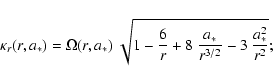
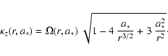
We have the following ordering:
| (55) | |||
| (56) |
The eigenvalues for the density waves are shown with decreasing
magnitude in Table 1. This holds for a neutron
star with angular velocity
![]() .
We
compared the Newtonian case with the Schwarzschild metric. The highest
speed pattern, given by
.
We
compared the Newtonian case with the Schwarzschild metric. The highest
speed pattern, given by ![]() ,
never exceeds the orbital
frequency at the ISCO. Note that in the m=1 case, the inner Lindblad
resonance does not exist for the Newtonian potential, and only a few
free wave solutions can be found for the Schwarzschild geometry.
,
never exceeds the orbital
frequency at the ISCO. Note that in the m=1 case, the inner Lindblad
resonance does not exist for the Newtonian potential, and only a few
free wave solutions can be found for the Schwarzschild geometry.
Table 1:
The first eight largest eigenvalues ![]() for
the free wave solutions of Eq. (43).
Values are normalized to the frequency of the ISCO,
for
the free wave solutions of Eq. (43).
Values are normalized to the frequency of the ISCO,
![]() .
Results are given for 3 azimuthal modes m=1,2,5 for
the Newtonian, as well as for the Schwarzschild gravitational field.
Where no inner Lindblad resonance exist, this is represented by -.
.
Results are given for 3 azimuthal modes m=1,2,5 for
the Newtonian, as well as for the Schwarzschild gravitational field.
Where no inner Lindblad resonance exist, this is represented by -.
Some examples of the corresponding eigenfunctions for density waves are shown in Fig. 1 with arbitrary normalization. Each of them possesses its own inner Lindblad radius depending on the eigenvalue. They are distinguished by the number of radial nodes they possess, starting from no node at all, which corresponds to the highest speed pattern.
![\begin{figure}
\par\begin{tabular}{cc}
\includegraphics[width=3.8cm,clip]{1511f...
...ps} &
\includegraphics[width=3.7cm,clip]{1511f4.eps} \end{tabular} \end{figure}](/articles/aa/full/2005/32/aa1511-04/img197.gif) |
Figure 1: Density wave perturbation in the disk caused by the free wave propagation for the azimuthal mode m=2. Some examples are shown for different eigenvalues and for Newtonian geometry, on the left, as well as for Schwarzschild geometry, on the right. The vertical bar indicates the location of the inner Lindblad resonance. The normalization of the eigenfunctions is arbitrary. |
| Open with DEXTER | |
Because the pattern speed of the first spiral waves is close to the ISCO, we suggest that these free wave solutions can be associated with the highest kHz QPO. More precisely, there exists one eigenfunction which possesses no root, namely the one with the highest eigenvalue. Eigenfunctions with several nodes in the radial distribution will emit no significant radiation since on average the fluctuations will cancel out. Therefore, we expect to see only density fluctuations with no or very few radial nodes. The most interesting candidate is the one with no node, a situation that also corresponds to the highest eigenvalue.
Moreover, while propagating in the perturbed rotating gravitational
field of the star, this spiral wave experiences a sinusoidally varying
gravity at a rate
![]() ,
where
,
where
![]() is the speed
pattern of the wave. This induces a modulation in the shape of the
wave which will be reflected in the power spectrum density as a kind of
beat phenomenon. As a result, in our model, we associate the highest
kHz-QPO to
is the speed
pattern of the wave. This induces a modulation in the shape of the
wave which will be reflected in the power spectrum density as a kind of
beat phenomenon. As a result, in our model, we associate the highest
kHz-QPO to
![]() and the lowest kHz QPO to the beat
frequency
and the lowest kHz QPO to the beat
frequency
![]() .
The peak separation is then
.
The peak separation is then
![]() .
.
In a real accretion disk, the precise location of the inner edge does
not necessarily reach the ISCO. The magnetic field or the radiation
pressure can prevent the disk from doing so. Indeed, the boundary of
the inner part of the disk can fluctuate due to the varying accretion
rate. For instance when the accretion process is enhanced, the inner
edge moves closer to the ISCO. As a result, the highest eigenvalue of
the free waves also increases and therefore ![]() shifts to higher
frequencies as well as
shifts to higher
frequencies as well as ![]() .
.
Examples of this mechanism are shown in Fig. 2. We
estimate the highest eigenvalue for the modes m=2,5 in the
Newtonian, as well as in the Schwarzschild gravitational potential.
The pattern speed of the wave solution
![]() ,
normalized to the
frequency of the ISCO,
,
normalized to the
frequency of the ISCO,
![]() ,
is shown as a function of the
location of the inner boundary of the accretion disk
,
is shown as a function of the
location of the inner boundary of the accretion disk
![]() .
In each
case, we observe an increase in the eigenvalue when the disk's inner
edge moves closer to the compact object, corresponding to an increased
accretion rate. When the ISCO is reached, the boundary condition does
not change anymore and the eigenvalue saturates to its final value.
Thus the kHz-QPO frequencies associated with the speed pattern of the
wave saturate. This has been observed in some LMXBs, as reported for
instance in a paper by Zhang et al. (1998).
.
In each
case, we observe an increase in the eigenvalue when the disk's inner
edge moves closer to the compact object, corresponding to an increased
accretion rate. When the ISCO is reached, the boundary condition does
not change anymore and the eigenvalue saturates to its final value.
Thus the kHz-QPO frequencies associated with the speed pattern of the
wave saturate. This has been observed in some LMXBs, as reported for
instance in a paper by Zhang et al. (1998).
| |
Figure 2:
Variation of the highest eigenvalue, corresponding to
the eigenfunction having no node, as a function of the location of
the inner edge of the disk
|
| Open with DEXTER | |
We now solve the full inhomogeneous Eq. (40) in order
to find the solution corresponding to the non-wavelike perturbation.
In this case, the eigenvalue is known:
![]() .
We
have to solve the second order ordinary differential equation
for
.
We
have to solve the second order ordinary differential equation
for ![]() with the appropriate boundary conditions
Eq. (51). Following the results given in
Appendix B, the most general solution is:
with the appropriate boundary conditions
Eq. (51). Following the results given in
Appendix B, the most general solution is:
| |
Figure 3: Non-wavelike disturbance in the inner part of the accretion disk due to the asymmetric component of the magnetic field. The potential is Newtonian and m=2. The numerical values used are described in Sect. 5. |
| Open with DEXTER | |
The counterrotating disk can be solved in exactly the same way by integrating Eq. (40) to find the solution corresponding to the non-wavelike perturbation. The amplitude of the oscillations is shown in Fig. 4. The Lindblad resonances are no longer in the computational domain. An oscillatory structure appears in the whole disk. The maximum amplitude is about 1% of the average density. This can later be compared with the numerical simulations.
| |
Figure 4: Non-wavelike disturbance in the inner part of the accretion disk due to the asymmetric component of the magnetic field. The potential is Newtonian, m=2 and the disk is counterrotating. |
| Open with DEXTER | |
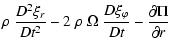
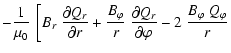
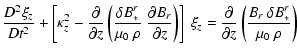
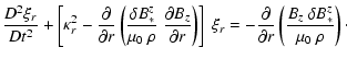
To get more insight into the nature of the resonances, we now focus on the displacement of the disk either in the equatorial plane or perpendicular to it. This means that we neglect the coupling between the oscillations occurring in perpendicular directions. This simplification will help us to understand the origin of the instability and to derive some resonance conditions.
To study the motion in the vertical direction, setting
![]() we find:
we find:
 |
(60) | ||
| (61) |
Further, we neglect the magneto-acoustic wave propagation because of
the weakly magnetized thin disk approximation, and also assume a
homogeneous medium for which the vertical Lagrangian displacement and
density are independent of the altitude z in the first case and
where the density and radial Lagrangian displacement do not depend on
the radius r in the second case. Note also that terms like
![]() are second order with respect to the perturbation and
should be neglected. These simplifications make the equations much
more easier to manipulate without losing the most interesting physical
aspect contained in the resonance terms. We can then simplified
Eqs. (59) and (62) to obtain:
are second order with respect to the perturbation and
should be neglected. These simplifications make the equations much
more easier to manipulate without losing the most interesting physical
aspect contained in the resonance terms. We can then simplified
Eqs. (59) and (62) to obtain:
| , | (65) |
The equation satisfied by each component of the Lagrangian
displacement when looking at a given azimuth ![]() is therefore
in the form:
is therefore
in the form:
From this analysis we expect three kinds of resonances corresponding to, (see Appendix C for a detailed analysis):
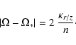
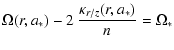
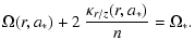
More generally, for a perturbation of arbitrary azimuthal mode m, the resonance conditions are given by:
From the resonance conditions derived previously,
Eqs. (67)-(69), we can estimate the radii
where each of these resonances occurs. Beginning with the Newtonian
potential, it is well known that the angular velocity, the radial and
epicyclic frequencies are all equal. For a weakly magnetized thin
accretion disk, this statement remains true so that
![]() .
Distinguishing between the two signs of
the absolute value, we get the following rotation rate for the
parametric condition (69):
.
Distinguishing between the two signs of
the absolute value, we get the following rotation rate for the
parametric condition (69):
| (70) | |||
| (71) |
Table 2:
Value of the orbital frequencies at the parametric
resonance radii for the first five orders n in the case of a
Newtonian gravitational potential. The results are given for
a
![]() neutron star rotating at 300 and
neutron star rotating at 300 and
![]() respectively. The value to the left of the symbol / corresponds
to the absolute value sign taken to be - and on the right to
be +. The -- sign indicates that no resonance condition can be satisfied.
respectively. The value to the left of the symbol / corresponds
to the absolute value sign taken to be - and on the right to
be +. The -- sign indicates that no resonance condition can be satisfied.
The parametric resonance condition Eq. (69), split into
the two cases depending on the sign of the absolute value, becomes:
Table 3:
Value of the orbital frequencies at the parametric
resonance radii for the first five orders n in the general
relativistic case. The results are given for a
![]() neutron star rotating at 300 and
neutron star rotating at 300 and
![]() respectively. The
value to the left of the symbol / corresponds to the absolute
value sign taken to be - and on the right to be +.
respectively. The
value to the left of the symbol / corresponds to the absolute
value sign taken to be - and on the right to be +.
We have now overcome the problem faced in the Newtonian approximation. Indeed, even in the case of a 300 Hz spinning neutron star, we can expect frequencies as high as 1332 Hz for the n=1 rank, in accordance with observations. The general-relativistic effect caused by the presence of the ISCO is therefore a crucial characteristic that makes a clear distinction with the Newtonian potential. The ISCO has to be implemented in any realistic QPO model in order to get a good quantitative agreement with observations. Therefore, a fully general-relativistic simulation code should be developed in order to take this ISCO into account in a self-consistent manner. However, we point out that general relativistic effects are not directly responsible for the observed QPOs as claimed in other models (Lee et al. 2004; Stella et al. 1999). They merely lead to quantitative improvements compared to the flat spacetime results.
The linear analysis described above is not the end of the story. It was shown that the disk becomes unstable at some preferred radii where the resonance conditions are satisfied. But this analysis does not tell us what will happen to these resonances on a long time scale. Moreover, as in the hydrodynamical case, the non-linearities in the time evolution of the disk will give rise to a rich variety of physical processes. However, in this simulation, in order to check our numerical algorithm, we start with runs for which the perturbation remains weak, in order to keep a regime close to the linear one described in the previous section. The full non-linear effects arising from a strong magnetic field perturbation will be treated in a forthcoming paper.
To achieve this goal, we performed 2D numerical simulations by solving the magnetohydrodynamical equations for the accretion disk Eqs. (15)-(19). This is done by a pseudo-spectral method for a simplified version of the 2D MHD accretion disk. Indeed, an exact treatment of the magnetic field induced by the motions in the disk would involve solution of an elliptic partial differential equation related to Ampere's law. We don't want to go into such refinement in this paper but only emphasize the role of a rotating asymmetric magnetic field. Nevertheless the physics at hand remains the same.
We expand every quantity in Fourier series in the azimuthal direction
and in Tchebyshev series in the radial direction, whereas time
integration is performed by an explicit fourth-order Runge-Kutta
scheme. In this work we are not interested in the accretion process
itself but focus only on the oscillations occurring in this system
around its stationary state. We can then impose fixed boundary
conditions in the radial direction by setting the radial velocity
equal to zero at the two boundaries. Furthermore, to avoid spurious
reflections at the edges of the accretion disk, we force the radial
velocity to decrease to zero in a narrow layer around these
boundaries. We also require the density and the azimuthal velocity to
reach their equilibrium. This acts as an ad hoc absorption process
damping out the strong oscillations which could arise in these
regions. The non-reflecting boundaries conditions are therefore
expressed as:
We adopted the geometry of a cylinder of gas threaded by a vertical
magnetic field and a radially directed gravitational field. The
problem is invariant under translation in the direction of the
magnetic field lines, which is chosen to be the z direction,
![]() .
Motions of the gas are only allowed in the
equatorial plane
.
Motions of the gas are only allowed in the
equatorial plane
![]() ,
vz=0; therefore, we suppress the
possibility of a warped disk and a possible precession of its orbital
plane, leaving this to future work. The ideal MHD
Eqs. (15) and (16) then simplify
to:
,
vz=0; therefore, we suppress the
possibility of a warped disk and a possible precession of its orbital
plane, leaving this to future work. The ideal MHD
Eqs. (15) and (16) then simplify
to:
 |
= | 0 | (82) |
| = | 0 | (83) | |
| = | 0 . | (84) |
| jr | = |  |
(86) |
| = |  |
(87) | |
| jz | = | 0 . | (88) |
We use geometrized units in which G=c=1. Distance is measured in
units of the gravitational radius given by
![]() .
Moreover, the simulations are done for a star with M*=1, so that in
the new units we have
.
Moreover, the simulations are done for a star with M*=1, so that in
the new units we have
![]() .
The star is assumed to be perfectly
spherical with the three main axes all equal
Rx=Ry=Rz, and the
perturbation comes from the magnetic field alone. The adiabatic
constant is equal to
.
The star is assumed to be perfectly
spherical with the three main axes all equal
Rx=Ry=Rz, and the
perturbation comes from the magnetic field alone. The adiabatic
constant is equal to
![]() and typical resolution
is
and typical resolution
is
![]() .
.
We checked that this resolution is sufficient by running a simulation
with twice as many points in both directions, namely
![]() .
We
found no changes in the solutions. Indeed inspecting the
Fourier-Tchebyshev coefficients, only half of the radial coefficients
and a few of the azimuthal coefficients in the 2D expansions are
significantly different from zero. Choosing a higher resolution will
not lead to any improvement in the solution but only to excessive
computation time.
.
We
found no changes in the solutions. Indeed inspecting the
Fourier-Tchebyshev coefficients, only half of the radial coefficients
and a few of the azimuthal coefficients in the 2D expansions are
significantly different from zero. Choosing a higher resolution will
not lead to any improvement in the solution but only to excessive
computation time.
The initial density profile is prescribed as
With these prescribed initial conditions, the thin disk approximation
is fairly good. Indeed the disk ratio H/R, H typical height and
R radius of the disk, plotted for the Newtonian and Schwarzschild
geometry in Fig. 5, never exceed 0.1 in any run.
Moreover, the disk is threaded by a weak magnetic field except very
close to the inner edge. The plasma ![]() parameter is shown in
Fig. 6 and remains very high.
parameter is shown in
Fig. 6 and remains very high.
| |
Figure 5: Thin disk approximation in which the ratio H/R never exceeds 0.1, on the left for the Newtonian potential and on the right for the Schwarzschild geometry. |
| Open with DEXTER | |
| |
Figure 6:
Plasma |
| Open with DEXTER | |
Before the time t=0, the disk stays in its axisymmetric equilibrium state and possesses only an azimuthal motion. At t=0, we switch on the perturbation by adding an asymmetric rotating component to the magnetic field. We then let the system evolve during more than one thousand orbital revolutions of the inner edge of the disk. We performed four sets of simulations. In the first one, the gravitational potential was Newtonian. In the second, we used a pseudo-Newtonian potential in order to take the ISCO into account. This is well-suited to describing the Schwarzschild space-time. In the third one, we took the angular momentum of the star into account by introducing a pseudo-Kerr geometry. And finally in the fourth and last set, we performed simulations with a counter rotating accretion disk evolving in the Newtonian potential described in the first set.
We have tested the pseudo-spectral method used in this paper on some standard problems. For instance, we solved the Euler equations in cylindrical coordinates for an initial jump in the density profile and retrieved the classical results of the shock problem with the correct shock speed. However, in order to reduce the oscillations (Gibbs phenomenon) due to discontinuity at the shock, we filtered out the high frequency components in Fourier-Tchebyshev space.
In a second set of tests, we launched an m=1 free wave in the
magnetized accretion disk, without any perturbation in the magnetic
field. The wave is slowly damped due to the absorbing boundary
conditions. The linear analysis elaborated in the previous section is
in agreement with the non-linear simulations presented below, at least
when the perturbations in the variables
![]() remain small. For problems without shock or discontinuity in the flow,
this pseudo-spectral code gives very accurate solutions with only a few
discretization points.
remain small. For problems without shock or discontinuity in the flow,
this pseudo-spectral code gives very accurate solutions with only a few
discretization points.
First, we study the behavior of the disk in the Newtonian potential.
In this case, the Keplerian rotation rate, the vertical and the radial
epicyclic frequencies for a single particle are all identical.
However, for a thin gaseous disk, there is a slight difference on the
order H/R and we have:
| (94) |
![\begin{figure}
\par\includegraphics[width=7.4cm,clip]{1511f12.eps} \end{figure}](/articles/aa/full/2005/32/aa1511-04/img299.gif) |
Figure 7:
Final snapshot of the density perturbation
|
| Open with DEXTER | |
The final snapshot of the density perturbation in the disk calculated
as
![]() is shown in
Fig. 7. We clearly recognize the spatial
separation between the propagating and non-propagating regions
delimited by the inner Lindblad resonance located at
is shown in
Fig. 7. We clearly recognize the spatial
separation between the propagating and non-propagating regions
delimited by the inner Lindblad resonance located at
![]() .
However, the outer Lindblad resonance at
.
However, the outer Lindblad resonance at
![]() is not seen
in this run because the magnetic perturbation close to the outer
boundary is very weak compared to its amplitude close to the inner
edge. The corotation resonance, located in the neighborhood
of r=40.0, is also not apparent. The reason is that its growth rate
is linear and very weak; an estimate is found by taking the typical
driven resonance for a harmonic oscillator as
is not seen
in this run because the magnetic perturbation close to the outer
boundary is very weak compared to its amplitude close to the inner
edge. The corotation resonance, located in the neighborhood
of r=40.0, is also not apparent. The reason is that its growth rate
is linear and very weak; an estimate is found by taking the typical
driven resonance for a harmonic oscillator as
 |
(96) |
![\begin{figure}
\par\includegraphics[width=7cm,clip]{1511f13.eps} \end{figure}](/articles/aa/full/2005/32/aa1511-04/img308.gif) |
Figure 8:
Cross section of the density perturbation
|
| Open with DEXTER | |
| |
Figure 9:
Amplitude of the Fourier components of the density perturbation.
The odd modes are numerically zero. Due to small nonlinearities,
the even modes are apparent but with weak amplitude. The
components |
| Open with DEXTER | |
The nonlinearities are weak throughout the simulation. Indeed,
looking at the Fourier spectrum of the density in
Fig. 9, the amplitude of each component,
plotted vs. the mode m on a logarithmic scale, is small except for
that corresponding to the excitation mode. The odd modes are not
present. However, the weak nonlinearities create a cascade to high
even modes starting with m=2. The largest asymmetric expansion
coefficient Cm is m=2, while the next even coefficients roughly
follow a geometric series with a factor q=10-3, so we can write
for all m even,
![]() ,
until they reach
values less than 10-20, which can be interpreted as zero from a
numerical point of view. As deviation from the stationary state is
weak, the amplitudes of these even modes decay compared to the
previous one, the highest being of course m=2. Thus, even in the
full non-linear simulation, the regime remains quasi-linear.
Consequently, the parametric resonance phenomenon discussed in the
previous section is irrelevant at this stage of our work. The effects
of strong nonlinearity will be studied in a forthcoming paper. Note
that due to the desaliasing process, the modes
,
until they reach
values less than 10-20, which can be interpreted as zero from a
numerical point of view. As deviation from the stationary state is
weak, the amplitudes of these even modes decay compared to the
previous one, the highest being of course m=2. Thus, even in the
full non-linear simulation, the regime remains quasi-linear.
Consequently, the parametric resonance phenomenon discussed in the
previous section is irrelevant at this stage of our work. The effects
of strong nonlinearity will be studied in a forthcoming paper. Note
that due to the desaliasing process, the modes ![]() are all set to
zero. Note also that the free wave solutions leave the computational
domain and do not return. Only the non-wavelike disturbance produces
significant changes in the density profile.
are all set to
zero. Note also that the free wave solutions leave the computational
domain and do not return. Only the non-wavelike disturbance produces
significant changes in the density profile.
![\begin{figure}
\par\includegraphics[width=7.4cm,clip]{1511f15.eps} \end{figure}](/articles/aa/full/2005/32/aa1511-04/img311.gif) |
Figure 10: Same as in Fig. 7 but the Newtonian potential is replaced by a pseudo-Schwarzschild one. |
| Open with DEXTER | |
In order to take into account the modification of the radial epicyclic
frequency due to the curved space-time around a Schwarzschild black
hole, we replaced the Newtonian potential by the logarithmically
modified potential proposed by Mukhopadhyay (2003).
This potential is well-suited to approximating the angular and
epicyclic frequencies in accretion disks around a rotating black hole.
The radial gravitational field derived from this potential is given
by
| Rms | = | (98) | |
| Z1 | = | 1 + (1-a2)1/3 [ (1+a)1/3 + (1-a)1/3 ] | (99) |
| Z2 | = | (100) |
The important feature of this potential is that the radial epicyclic frequency for a single particle vanishes at the innermost stable circular orbit (ISCO), which implies that the parametric resonance condition can be fulfilled in the very inner part of the accretion disk for different values of the integer n but still with a very small radial extension. However, due to the small perturbation we remain in the linear regime, and the parametric resonance is only of second order. The disk boundaries, the star rotation rate, and the normalization are the same as in the previous case.
The final snapshot of the density perturbation in the disk is shown in
Fig. 10. The corotation resonance is now located
at r=43.7, which differs slightly from the previous simulation
because the orbital velocity is no longer Keplerian due to the
pseudo-Newtonian force Eq. (97). The
non-wavelike disturbance exists between the inner edge of the disk and
the inner Lindblad resonance. By viewing a cross section, the Lindblad
radii appear clearly as seen in Fig. 11.
Inspection of the Fourier coefficients of the density
Fig. 12 proves that the linear regime is
preserved. The level of excitation of the even modes ![]() is very
weak.
is very
weak.
| |
Figure 11:
Same as in Fig. 8 but
for the pseudo-Schwarzschild potential. The Lindblad resonances
are located at
|
| Open with DEXTER | |
| |
Figure 12: Same as Fig. 9 but for the pseudo-Schwarzschild potential. The Fourier coefficients form a decaying geometric series. |
| Open with DEXTER | |
![\begin{figure}
\par\includegraphics[width=7.4cm,clip]{1511f18.eps} \end{figure}](/articles/aa/full/2005/32/aa1511-04/img318.gif) |
Figure 13: Same as in Fig. 10 but with an azimuthal mode m=1. |
| Open with DEXTER | |
![\begin{figure}
\par\includegraphics[width=7cm,clip]{1511f19.eps} \end{figure}](/articles/aa/full/2005/32/aa1511-04/img319.gif) |
Figure 14:
Same as in Fig. 11 but
with an azimuthal mode m=1. The Lindblad resonances are located
at
|
| Open with DEXTER | |
| |
Figure 15: Same as Fig. 12 but with an azimuthal mode m=1. The Fourier coefficients form a decaying geometric series. |
| Open with DEXTER | |
The results of replacing the m=2 mode by a more realistic m=1mode, in accordance with the dipolar structure of the magnetic field,
is shown in Fig. 13.
The inner Lindblad resonance moves closer to the inner edge and is
located at
![]() .
There is less space left for the
non-wavelike disturbance between the inner edge and the inner Lindblad
resonance as can be seen in Fig. 14.
Also, all the azimuthal modes are now excited starting with m=1 and
with decreasing magnitude, Fig. 15.
From a qualitative point of view, we can draw the same conclusions as
in the case of the Newtonian disk. The absence or presence of the ISCO
does not affect the physics of the resonances, but only has an effect
on their amplitude and their location.
.
There is less space left for the
non-wavelike disturbance between the inner edge and the inner Lindblad
resonance as can be seen in Fig. 14.
Also, all the azimuthal modes are now excited starting with m=1 and
with decreasing magnitude, Fig. 15.
From a qualitative point of view, we can draw the same conclusions as
in the case of the Newtonian disk. The absence or presence of the ISCO
does not affect the physics of the resonances, but only has an effect
on their amplitude and their location.
We also ran a simulation in which the rotation of the star is taken into account. This shifts the location of the ISCO closer to the surface of the neutron star.
We chose a star with an angular momentum of a*=0.5. Therefore, the
disk inner boundary corresponding to the marginally stable circular
orbit will be located at R1=4.24, while the outer boundary is chosen
to be at R2=42.4. The star magnetic perturbation in this run is ten
times larger than in the previous case,
![]() .
Therefore
the computation starts to leave the linear regime and reaches a weak
non-linear state.
.
Therefore
the computation starts to leave the linear regime and reaches a weak
non-linear state.
The corotation resonance at r=23.8 is not reached, as can be seen from Fig. 16. However, the wave and non-wavelike disturbances are clearly identified between the inner edge and the inner Lindblad resonance. They persist during the whole simulation at the low level predicted by the linear analysis. The precise location of the Lindblad resonance is determined by the cross section view shown in Fig. 17. Looking at the Fourier components in Fig. 18, all the even modes are excited at a substantial level. The stronger stellar perturbation starts to excite modes which are multiples of the injection scale given by m=2.
![\begin{figure}
\par\includegraphics[width=7.4cm,clip]{1511f21.eps} \end{figure}](/articles/aa/full/2005/32/aa1511-04/img323.gif) |
Figure 16: Final snapshot of the density perturbation in the accretion disk evolving in a perturbed pseudo-Kerr potential with a=0.5. The disk extends from R1=4.24 to R2=42.4. The outer Lindblad resonance is not on the grid. |
| Open with DEXTER | |
| |
Figure 17:
Same as in Fig. 8 but
for the pseudo-Kerr potential. The inner Lindblad resonance
appears clearly at
|
| Open with DEXTER | |
| |
Figure 18: Same as Fig. 9 but for the pseudo-Kerr potential. |
| Open with DEXTER | |
Finally we checked that the Lindblad resonances disappear for a
retrograde Newtonian disk. The numerical values are the same as in
Sect. 5.3, except that the sign of the stellar spin is
taken to be
![]() and the magnetic
perturbation
and the magnetic
perturbation
![]() .
.
Looking at Fig. 19, the evolution of the disk does not show any Lindblad resonance as expected. The mode m=2 with two spiral arms propagates in the whole computational domain. The disk reaches a quasi-stationary state in which the density fluctuations are well established, Fig. 20. They fit the shape found in the linear analysis, Fig. 4. Again, the stronger stellar magnetic perturbation affects the high order azimuthal modes, which are excited at the same amplitude as the injection mode m=2, Fig. 21.
![\begin{figure}
\par\includegraphics[width=7.4cm,clip]{1511f24.eps} \end{figure}](/articles/aa/full/2005/32/aa1511-04/img327.gif) |
Figure 19:
Final snapshot of the density perturbation in
the counterrotating accretion disk evolving in a perturbed
Newtonian potential. Same values as in
Fig. 7 apply except for the sign
of |
| Open with DEXTER | |
![\begin{figure}
\par\includegraphics[width=7cm,clip]{1511f25.eps} \end{figure}](/articles/aa/full/2005/32/aa1511-04/img328.gif) |
Figure 20: Same as Fig. 8 but for the retrograde disk. The Lindblad resonances are no longer present. |
| Open with DEXTER | |
| |
Figure 21: Same as Fig. 9 but with a retrograde disk. |
| Open with DEXTER | |
Here also we can replace the m=2 mode by a more realistic m=1 one,
in accordance with the dipolar structure of the magnetic field and
with, for example, a smaller magnetic perturbation taken again to
be
![]() .
The results for the density perturbation are
shown in Fig. 22. A spiral wave is formed and
propagates in the whole disk with a rotation rate equal to the neutron
star spin.
Now all the Fourier components are excited, the strongest one
corresponds to m=1, and the lighter order ones have decreasing
amplitudes, as shown in Fig. 24.
.
The results for the density perturbation are
shown in Fig. 22. A spiral wave is formed and
propagates in the whole disk with a rotation rate equal to the neutron
star spin.
Now all the Fourier components are excited, the strongest one
corresponds to m=1, and the lighter order ones have decreasing
amplitudes, as shown in Fig. 24.
![\begin{figure}
\par\includegraphics[width=7.4cm,clip]{1511f27.eps} \end{figure}](/articles/aa/full/2005/32/aa1511-04/img331.gif) |
Figure 22:
Final snapshot of the density perturbation in
the counterrotating accretion disk evolving in a perturbed
Newtonian potential. Same values as in the
Fig. 7 caption excepted for the sign
of |
| Open with DEXTER | |
![\begin{figure}
\par\includegraphics[width=7cm,clip]{1511f28.eps} \end{figure}](/articles/aa/full/2005/32/aa1511-04/img332.gif) |
Figure 23: Same as Fig. 8 but with a retrograde disk. The Lindblad resonances have disappeared. |
| Open with DEXTER | |
| |
Figure 24: Same as Fig. 9 but with a retrograde disk. |
| Open with DEXTER | |
To summarize, in all of the results obtained by these runs, the exact structure of the gravitational potential, be it Newtonian or pseudo-Newtonian, does not affect the physics of the resonances. The main features of these resonances are their location very close to the inner boundary of the accretion disk. When the applied magnetic asymmetry is small enough, the perturbations remain in the linear regime.
In this paper, we studied the effects of an asymmetric rotating dipolar or multipolar magnetic field on a magnetized accretion disk. This situation is well-suited to LMXBs containing a neutron star, since they are believed to possess a magnetic field that more or less channels the accreting matter to the polar caps of the neutron star, depending on its strength. The same conclusions can be drawn in the case of a hydrodynamical disk evolving in a quadrupolar gravitational potential perturbation. Although the flows differ, the consequences of a rotating asymmetric field are qualitatively the same. The disk is subject to the corotation resonance, the Lindblad driven resonances, and if the perturbation is strong enough, the parametric instability. We derived an explicit formulation for the regions where the blobs should form, given by the resonance conditions Eqs. (67)-(69). On the one hand, these blobs can persist during thousands of orbital revolutions and can account for the high quality factor Q seen in some high frequency-QPOs. On the other, the pattern speed of the free wave solutions is closely related to the location of the inner boundary of the accretion disk. The observed shift in the HFQPOs in response to the accretion rate can be explained by these solutions.
This study should be extended to include viscosity of the gas flowing in the disk, which should set a lower limit to the magnetic field perturbation amplitude in order to have parametric resonance. In addition, the loss of energy by radiation should also damp these oscillations and select only a few of them, which will also permit estimation of the light curves of such systems. The relation between the simulations presented in this paper and observations will be investigated in a forthcoming paper, in which we show how to calculate the power spectrum density (PSD) of the accretion disk. The prediction of the PSD will be crucial for validation of the model.
We would like to emphasize that this work is only a preliminary study undertaken to prove that a rotating asymmetric magnetic field leads to some interesting resonance mechanisms. The toy model used here cannot be applied directly to observations. Indeed, many aspects, such as the warping/precession of the disk expected in 3D simulations, as well as viscosity and radiation, should be taken into account in a more realistic model.
Nevertheless, we believe that this idea can also be applied to the LMXBs containing a black hole. Indeed, it seems that the existence of QPOs in black hole candidates is correlated with the detection of a jet emanating from these systems, (McClintock & Remillard 2003). The Blandford-Znajek process (Blandford & Znajek 1977) converting the rotational energy of the black hole into the launching of the jet should also be responsible for a connection between the accretion disk and the black hole via the magnetic field. Therefore, the model presented in this paper has the potential to explain the QPOs seen in the BHCs (Wang et al. 2003).
Acknowledgements
This research was carried out in an FOM projectruimte on "Magnetoseismology of accretion disks'', a collaborative project between R. Keppens (FOM Institute Rijnhuizen, Nieuwegein) and N. Langer (Astronomical Institute Utrecht). This work is part of the research programme of the "Stichting voor Fundamenteel Onderzoek der Materie (FOM)'', which is financially supported by the "Nederlandse Organisatie voor Wetenschappelijk Onderzoek (NWO)''.
I am grateful to the referee Lev Titarchuk for his valuable comments and remarks as well as to Jean Heyvaerts and John Kirk for carefully reading the manuscript.
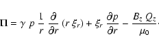
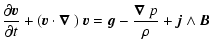
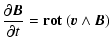
The linearization of the MHD equations is done by introducing the
Lagrangian displacement vector ![]() ,
which is related to the
Eulerian and Lagrangian perturbation of the fluid physical quantities,
such as the velocity, the magnetic field, and the density. These
perturbations are denoted respectively by
,
which is related to the
Eulerian and Lagrangian perturbation of the fluid physical quantities,
such as the velocity, the magnetic field, and the density. These
perturbations are denoted respectively by ![]() and
and ![]() .
By
definition, the Lagrangian perturbation of the velocity is
.
By
definition, the Lagrangian perturbation of the velocity is
 |
(A.1) |
| (A.2) |
Let's start by perturbing the mass conservation equation by using the
equilibrium condition
![]()
 |
(A.7) |
 |
(A.8) |
| (A.9) |
 |
(A.10) |
| |
= |  |
|
| (A.11) | |||
| = |  |
||
| (A.12) | |||
| = |  |
||
| (A.13) |
 |
(A.15) |
Finally for the pressure perturbation, we develop the adiabatic
condition to first order. We have
 |
(A.16) |
 |
(A.17) |
Replacing all the perturbed quantities by their expression involving
the Lagrangian displacement and keeping only the first order term,
![]() ,
satisfies a second order linear PDE given by
,
satisfies a second order linear PDE given by
 |
|||
| (A.19) |
| |
= |  |
(A.20) |
| = |  |
||
| (A.21) | |||
| = |  |
||
| (A.22) | |||
| = | (A.23) |
|
|||
![$\displaystyle \rho_0 ~ \frac{\partial^2\vec{\xi}}{\partial t^2}
+ 2 ~ \rho_0 ~ ...
... ) \vec{\xi} -
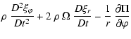
\rho_0 ~ \vec{\xi} ( \vec{v}_0 \cdot \nabla ) \vec{v}_0 \right].$](/articles/aa/full/2005/32/aa1511-04/img382.gif) |
(A.24) |
Recalling that
![]() and
and ![]() ,
we rewrite
,
we rewrite
| (A.25) |
In the stationary state, the disk orbits around the compact object
without mass in- or outflow from the edges and without precession.
From now on, we drop the subscript 0 for the stationary quantities,
which should not lead to any confusion. Thus the velocity in the
axisymmetric stationary state is simply
| |
= | (A.28) | |
| = | ![$\displaystyle \Omega ~
\left[ \left( \frac{\partial\xi_r}{\partial\varphi} - \x...
...) ~ \vec{e}_\varphi +
\frac{\partial\xi_z}{\partial\varphi} ~ \vec{e}_z \right]$](/articles/aa/full/2005/32/aa1511-04/img395.gif) |
||
| (A.29) | |||
| = | (A.30) |
| |
= |  |
(A.31) |
 |
|||
![$\displaystyle +
\left.
\left( \frac{\partial\xi_\varphi}{\partial\varphi} + \xi...
...) ~ \vec{e}_\varphi +
\frac{\partial\xi_z}{\partial\varphi} ~ \vec{e}_z
\right]$](/articles/aa/full/2005/32/aa1511-04/img401.gif) |
(A.32) | ||
| = |  |
(A.33) | |
| = | (A.34) |
| |
= |  |
(A.35) |
| = |  |
||
![$\displaystyle +
\left. \left( \frac{\partial^2 \xi_\varphi}{\partial\varphi^2} ...
...vec{e}_\varphi +
\frac{\partial^2 \xi_z}{\partial\varphi^2} ~ \vec{e}_z \right]$](/articles/aa/full/2005/32/aa1511-04/img408.gif) |
| |
= | ![$\displaystyle \left[ B_r ~ \frac{\partial Q_r}{\partial r} +
\frac{B_\varphi}{r...
...arphi~Q_\varphi}{r} +
B_z ~ \frac{\partial Q_r}{\partial z} \right] ~ \vec{e}_r$](/articles/aa/full/2005/32/aa1511-04/img410.gif) |
|
![$\displaystyle \quad + \left[ B_r ~ \frac{\partial Q_\varphi}{\partial r} +
\fra...
...Q_r}{r} +
B_z ~ \frac{\partial Q_\varphi}{\partial z} \right] ~ \vec{e}_\varphi$](/articles/aa/full/2005/32/aa1511-04/img411.gif) |
|||
![$\displaystyle \quad+ \left[ B_r ~ \frac{\partial Q_z}{\partial r} +
\frac{B_\va...
...}{\partial \varphi} +
B_z ~ \frac{\partial Q_z}{\partial z} \right] ~ \vec{e}_z$](/articles/aa/full/2005/32/aa1511-04/img412.gif) |
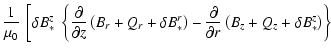
(A.36) |
| |
= | ![$\displaystyle \left[ Q_r ~ \frac{\partial B_r}{\partial r} +
\frac{Q_\varphi}{r...
...arphi~B_\varphi}{r} +
Q_z ~ \frac{\partial B_r}{\partial z} \right] ~ \vec{e}_r$](/articles/aa/full/2005/32/aa1511-04/img414.gif) |
|
![$\displaystyle \quad+ \left[ Q_r ~ \frac{\partial B_\varphi}{\partial r} +
\frac...
...B_r}{r} +
Q_z ~ \frac{\partial B_\varphi}{\partial z} \right] ~ \vec{e}_\varphi$](/articles/aa/full/2005/32/aa1511-04/img415.gif) |
|||
![$\displaystyle \quad+ \left[ Q_r ~ \frac{\partial B_z}{\partial r} +
\frac{Q_\va...
...}{\partial \varphi} +
Q_z ~ \frac{\partial B_z}{\partial z} \right] ~ \vec{e}_z$](/articles/aa/full/2005/32/aa1511-04/img416.gif) |
(A.37) |
| (A.38) | |||
| (A.39) |
 |
|||
 |
|||
 |
|||
![$\displaystyle -
\left.\left. \frac{\partial}{\partial\varphi} ( B_r + Q_r + \delta B_*^r ) \right\}
\right] ~ \vec{e}_r$](/articles/aa/full/2005/32/aa1511-04/img423.gif) |
|||
 |
|||
 |
|||
 |
|||
![$\displaystyle -
\left.\left. \frac{\partial}{\partial z}
( B_\varphi + Q_\varphi + \delta B_*^\varphi )\right\} \right] ~ \vec{e}_\varphi$](/articles/aa/full/2005/32/aa1511-04/img426.gif) |
|||
 |
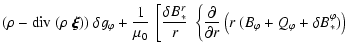
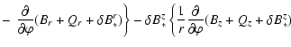
|||
 |
|||
 |
|||
![$\displaystyle -
\left.\left. \frac{\partial}{\partial r}
\left( B_z + Q_z + \delta B_*^z \right) \right\} \right] ~ \vec{e}_z$](/articles/aa/full/2005/32/aa1511-04/img429.gif) |
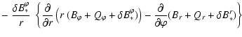
(A.40) |
 |
|||
![$\displaystyle -
\left.
\frac{B_\varphi + Q_\varphi}{r} ~ \left( \frac{\partial}...
...phi) -
\frac{\partial\delta B_*^r}{\partial\varphi} \right) \right] ~ \vec{e}_r$](/articles/aa/full/2005/32/aa1511-04/img431.gif) |
|||
 |
|||
![$\displaystyle -
\left. (B_z + Q_z) ~
\left( \frac{1}{r} ~ \frac{\partial\delta ...
...\frac{\partial\delta B_*^\varphi}{\partial z} \right) \right] ~ \vec{e}_\varphi$](/articles/aa/full/2005/32/aa1511-04/img433.gif) |
|||
 |
|||
![$\displaystyle -
\left.
(B_r + Q_r) \left( \frac{\partial\delta B_*^r}{\partial z} -
\frac{\partial\delta B_*^z}{\partial r} \right) \right] ~ \vec{e}_z.$](/articles/aa/full/2005/32/aa1511-04/img435.gif) |
(A.41) |
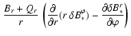
| Qr | = |  |
(A.42) |
| = |  |
(A.43) | |
| Qz | = | 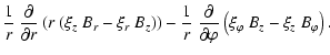 |
(A.44) |
 |
(A.45) |
To elucidate the meaning of these equations, we focus on the disk
response when motions in vertical direction and orbital plane are
decoupled. Let's start with the Lagrangian displacement contained in
the orbital plane of the disk by setting
![]() and
and ![]() .
We also assume that perturbations are axisymmetric
in order to avoid meaningless complications so that
.
We also assume that perturbations are axisymmetric
in order to avoid meaningless complications so that
![]() ,
corresponding to m=0 modes.
Then the magnetic perturbations read
,
corresponding to m=0 modes.
Then the magnetic perturbations read
| Qr | = | 0 | (A.49) |
| = | 0 | (A.50) | |
| Qz | = | 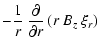 |
(A.51) |
 |
(A.52) |
| (A.56) | |||
 |
(A.57) |
| Qr | = |  |
(A.58) |
| = | 0 | (A.59) | |
| Qz | = | 0 | (A.60) |
 |
(A.61) |
 |
(A.63) |
In the numerical runs presented in this paper, we use non reflecting
boundary conditions which leads to a vanishing density perturbation at
the inner edge of the disk, namely
![]() .
In order to compare
the linear analysis with simulations, we adopt the same conditions in
the both cases. Neglecting the displacement in the vertical direction,
density perturbations are related to the Lagrangian displacement by
.
In order to compare
the linear analysis with simulations, we adopt the same conditions in
the both cases. Neglecting the displacement in the vertical direction,
density perturbations are related to the Lagrangian displacement by
 |
(A.64) |
 |
(A.65) |
 |
(A.67) |
In this appendix, we recall a method to find approximate solutions to
the following Schrödinger type equation with a source term f(x)
We start to look for solutions to the homogeneous part of
Eq. (B.1) when f(x)=0. The reference equation is
Airy's equation given by
It follows that
![]() .
The solution of
Eq. (B.11) is
.
The solution of
Eq. (B.11) is
Then
![]() .
The solution of Eq. (B.11) is
.
The solution of Eq. (B.11) is
Note that the function ![]() is strictly monotonic.
is strictly monotonic. ![]() never changes sign and never vanishes. Consequently, the amplitude Agiven by Eq. (B.10) remains finite in the entire
interval [a,b].
never changes sign and never vanishes. Consequently, the amplitude Agiven by Eq. (B.10) remains finite in the entire
interval [a,b].
Finally, two linearly independent solutions of the homogeneous part of
Eq. (B.1) can be expressed with help on the Airy
functions of the first and the second kind, respectively Ai and
Bi
Knowing the general solutions to the homogeneous part, a peculiar
solution to the full Eq. (B.1) with source term is
given by the formula
The corotation resonance is defined by the radius ![]() where
where
![]() .
Actually, this equation possesses two
solutions corresponding to
.
Actually, this equation possesses two
solutions corresponding to
![]() .
The width of this region is of the order of the disk height O(H).
For very thin disks, this discrepancy can be neglected and the two
solutions merge together in an unique corotation radius given
by
.
The width of this region is of the order of the disk height O(H).
For very thin disks, this discrepancy can be neglected and the two
solutions merge together in an unique corotation radius given
by
![]() .
In other words, we assume in this case
that
.
In other words, we assume in this case
that
![]() .
However, in our numerical application, the
separation between the two corotation radii is large enough to be
resolved. Nevertheless, in the derivation of the corotation resonance
below, we will assume that corotation is achieved
when
.
However, in our numerical application, the
separation between the two corotation radii is large enough to be
resolved. Nevertheless, in the derivation of the corotation resonance
below, we will assume that corotation is achieved
when
![]() .
For the detailed study
of both corotation, it can be shown that the leading term in the
equation satisfied by the radial displacement Eq. (25) is
given by
.
For the detailed study
of both corotation, it can be shown that the leading term in the
equation satisfied by the radial displacement Eq. (25) is
given by
| (C.4) |
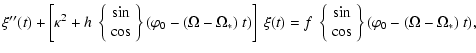
By choosing an appropriate origin of time t0, the generalized
Mathieu Eq. (66) can be recast in the more convenient
form as follows
When the amplitude of the modulation is weak compared to the driven
force ![]() ,
the parametric growth rate can be neglected. Indeed,
to this approximation, Eq. (C.13) reduce to the well
known driven harmonic oscillator
,
the parametric growth rate can be neglected. Indeed,
to this approximation, Eq. (C.13) reduce to the well
known driven harmonic oscillator
Note that the driven resonance (called Lindblad resonance in the main text to refer to the same physical process arising in galactic dynamic and described by Lindblad 1974) is a special case of the parametric resonance for n=2. As a consequence, we could enclose the driven resonance condition into the parametric one. Nevertheless, in order to keep track of the difference between linear and exponential growth rate, this distinction will remain throughout the paper. Moreover, in the numerical application shown in the simulations, the parametric resonance does not appear because of the weak magnetic field disturbance. The timescale of the growing parametric mode excess by several orders of magnitude the duration of the simulations. Only the Lindblad resonance is relevant in this case.

![$\displaystyle \frac{\mu_0}{4 ~ \pi} ~ \frac{\mu ~ \sin \chi}{(r^2+z^2)^{3/2}} ~
\left[ \frac{3~r^2}{r^2+z^2} - 1 \right] ~ \cos (\varphi-\Omega_*~t)$](/articles/aa/full/2005/32/aa1511-04/img63.gif)

![$\displaystyle \rho ~ \frac{D^2\vec{\xi}}{Dt^2}
- {\rm div}~\left[ \rho ~ \vec{\...
... ) \vec{v} \right] - \nabla\Pi
- \frac{1}{\mu_0} ~ \vec{B} \cdot \nabla \vec{Q}$](/articles/aa/full/2005/32/aa1511-04/img83.gif)
![$\displaystyle +
\left. B_z ~ \frac{\partial Q_r}{\partial z} + Q_r ~ \frac{\par...
...artial B_r}{\partial \varphi} +
Q_z ~ \frac{\partial B_r}{\partial z} \right] =$](/articles/aa/full/2005/32/aa1511-04/img96.gif)
![$\displaystyle -
\left.
\frac{B_\varphi + Q_\varphi}{r} ~ \left( \frac{\partial}...
...lta B_*^\varphi) -
\frac{\partial\delta B_*^r}{\partial\varphi} \right) \right]$](/articles/aa/full/2005/32/aa1511-04/img100.gif)
![$\displaystyle +
\left.
B_z ~ \frac{\partial Q_\varphi}{\partial z} + Q_r ~ \fra...
...\frac{Q_\varphi~B_r}{r} +
Q_z ~ \frac{\partial B_\varphi}{\partial z} \right] =$](/articles/aa/full/2005/32/aa1511-04/img103.gif)
![$\displaystyle -
\left. (B_z + Q_z) ~
\left( \frac{1}{r} ~ \frac{\partial\delta ...
...partial\varphi} -
\frac{\partial\delta B_*^\varphi}{\partial z} \right) \right]$](/articles/aa/full/2005/32/aa1511-04/img108.gif)
![$\displaystyle +
\left. Q_r ~ \frac{\partial B_z}{\partial r} +
\frac{Q_\varphi}...
... \frac{\partial B_z}{\partial z} \right] =
- {\rm div}~(\rho~\vec{\xi}) ) ~ g_z$](/articles/aa/full/2005/32/aa1511-04/img110.gif)
![$\displaystyle -
\left.
(B_r + Q_r) \left( \frac{\partial\delta B_*^r}{\partial z} -
\frac{\partial\delta B_*^z}{\partial r} \right) \right] \cdot$](/articles/aa/full/2005/32/aa1511-04/img115.gif)
![\begin{displaymath}
X(r,\varphi,t) = {\rm Re} [\tilde{X}(r) ~ {\rm e}^{{\rm i}(m~\varphi-\sigma~t)}],
\end{displaymath}](/articles/aa/full/2005/32/aa1511-04/img129.gif)
![$\displaystyle \tilde{\xi}_\varphi = - \frac{\rm i}{\omega_*^2} ~ \left[ - \frac...
...2}{r^2} ~ \frac{\partial}{\partial r}
\left( r ~ \tilde{\xi}_r \right) \right].$](/articles/aa/full/2005/32/aa1511-04/img142.gif)
![\begin{displaymath}
c_{{\rm ma}z}^2 ~ \left[ \frac{\partial^2\tilde{\xi}_r}{\pa...
... r} \right] +
( \omega^2 - \kappa_r^2) ~ \tilde{\xi}_r = 0 .
\end{displaymath}](/articles/aa/full/2005/32/aa1511-04/img156.gif)


![$\displaystyle g_r = - \frac{G~M_*}{r^2} \bigg[ 1 + R_{ms} \bigg( \frac{9}{20} ~...
...ac{R_{ms}-1}{r} - \frac{3}{2r} ~ \ln \frac{r}{(3r-R_{ms})^{2/9}} \bigg) \bigg],$](/articles/aa/full/2005/32/aa1511-04/img312.gif)
 = 0
= 0![$\displaystyle \rho_0 ~ \frac{\partial^2\vec{\xi}}{\partial t^2}
+ 2 ~ \rho_0 ~ ...
...a ) \vec{\xi} -
\rho_0 ~ \vec{\xi} ( \vec{v}_0 \cdot \nabla ) \vec{v}_0 \right]$](/articles/aa/full/2005/32/aa1511-04/img387.gif)
![$\displaystyle \quad-
\left.
2 ~ \frac{B_\varphi~Q_\varphi}{r} +
B_z ~ \frac{\pa...
...artial B_r}{\partial \varphi} +
Q_z ~ \frac{\partial B_r}{\partial z} \right] =$](/articles/aa/full/2005/32/aa1511-04/img442.gif)
![$\displaystyle \quad-
\left.
\frac{B_\varphi + Q_\varphi}{r} ~ \left( \frac{\par...
...*^\varphi) - \frac{\partial\delta B_*^r}{\partial\varphi} \right) \right] \cdot$](/articles/aa/full/2005/32/aa1511-04/img447.gif)
![$\displaystyle +
\left. Q_r ~ \frac{\partial B_\varphi}{\partial r} +
\frac{Q_\v...
...\frac{Q_\varphi~B_r}{r} +
Q_z ~ \frac{\partial B_\varphi}{\partial z} \right] =$](/articles/aa/full/2005/32/aa1511-04/img449.gif)
![$\displaystyle +
\left. Q_r ~ \frac{\partial B_z}{\partial r} +
\frac{Q_\varphi}...
...artial B_z}{\partial \varphi} +
Q_z ~ \frac{\partial B_z}{\partial z} \right] =$](/articles/aa/full/2005/32/aa1511-04/img453.gif)
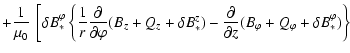

![$\displaystyle \rho ~ \frac{D^2\xi_r}{Dt^2} - \frac{\partial}{\partial r} \left[...
...t)
~ \frac{1}{r} ~ \frac{\partial}{\partial r} \left( r ~ \xi_r \right) \right]$](/articles/aa/full/2005/32/aa1511-04/img462.gif)
![$\displaystyle \rho ~ \frac{D^2\xi_z}{Dt^2} - \frac{\partial}{\partial z} \left[...
...0} \right)
\frac{\partial\xi_z}{\partial z} \right] +
\rho ~ \kappa_z^2 ~ \xi_z$](/articles/aa/full/2005/32/aa1511-04/img470.gif) =
= 
![\begin{displaymath}
\omega_1(x) = - \left[ \pm \frac{3}{2} ~ \int_0^x
\sqrt{p(s)} ~ {\rm d}s \right]^{2/3}.
\end{displaymath}](/articles/aa/full/2005/32/aa1511-04/img493.gif)
![\begin{displaymath}
\omega_1(x) = \left[ \pm \frac{3}{2} ~ \int_0^x
\sqrt{-p(s)} ~ {\rm d}s \right]^{2/3}.
\end{displaymath}](/articles/aa/full/2005/32/aa1511-04/img496.gif)
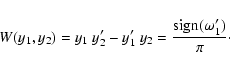
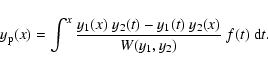

![$\displaystyle c_{{\rm ma}z}^2 ~ \left[ 1 + \frac{m^2~c_{{\rm ma}z}^2}{r^2~\omega_*^2} \right] ~
\frac{\partial^2\xi_r}{\partial r^2}$](/articles/aa/full/2005/32/aa1511-04/img510.gif)
![$\displaystyle +
\frac{c_{{\rm ma}z}^2}{r} ~ \left[
\frac{\partial \ln~(r~\rho~c...
...\partial}{\partial r}(\omega_*^{-2}) \right] ~
\frac{\partial\xi_r}{\partial r}$](/articles/aa/full/2005/32/aa1511-04/img511.gif)
![$\displaystyle +
\left[ \omega^2 - \kappa_r^2 + 4 ~ \Omega^2~
\left( 1 - \frac{\...
..._{{\rm ma}z}^2}{r} ~
\frac{\partial}{\partial r}(\omega_*^{-2}) \right] ~ \xi_r$](/articles/aa/full/2005/32/aa1511-04/img512.gif)
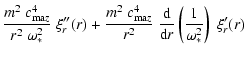
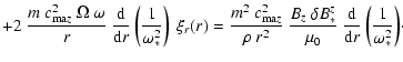

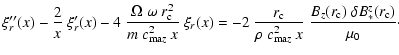
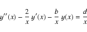
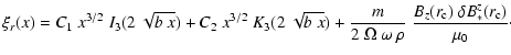
![\begin{displaymath}
\xi''(t) + \left[ \kappa^2 + h ~ \cos ( \gamma ~ t )
\right] ~ \xi(t) = f ~ \cos( \gamma ~ t )
\end{displaymath}](/articles/aa/full/2005/32/aa1511-04/img540.gif)