The decay rate of vertical kink waves in a curved flux tube is modeled numerically. The full MHD equations are solved for a curved equilibrium flux tube in an arcade geometry and the decay of
A&A 438, 733-740 (2005)
DOI: 10.1051/0004-6361:20042527
C. S. Brady - T. D. Arber
Physics Department, University of Warwick, CV4 7AL, Coventry, UK
Received 13 December 2004 / Accepted 11 April 2005
Abstract
The decay rate of vertical kink waves in a curved flux tube is modeled numerically.
The full
MHD equations are solved for a curved equilibrium flux tube in an
arcade geometry and the decay of ![]() ,
the integral over the flux tube of the
modulus of the velocity perpendicular to the local magnetic field, is
measured. These simulations are 2D and are thus restricted to kink oscillations in the
loop plane. The decay rate is
found to increase with increasing wavelength, increasing
,
the integral over the flux tube of the
modulus of the velocity perpendicular to the local magnetic field, is
measured. These simulations are 2D and are thus restricted to kink oscillations in the
loop plane. The decay rate is
found to increase with increasing wavelength, increasing ![]() and decreasing density contrast
ratio. The wave tunneling effect is shown to be a possible mechanism for
the high decay rate of the recent observed kink oscillation reported by Wang & Solanki (2004).
and decreasing density contrast
ratio. The wave tunneling effect is shown to be a possible mechanism for
the high decay rate of the recent observed kink oscillation reported by Wang & Solanki (2004).
Key words: Sun: corona - Sun: magnetic fields - Sun: oscillations
The first model of waves in flux tubes was created in response to radio observations and considered the linear eigenmodes of an isolated straight flux tube (Roberts et al. 1983, 1984). The results from this model show that a flux tube will act as a waveguide for fast magneto-acoustic waves, trapping the waves in regions of low Alfvén speed.
Models assuming that flux tubes are straight have been applied to coronal loops with some success (e.g. Nakariakov & Ofman 2001), but include an obvious simplification: the observed structures are strongly curved, with a radius of curvature that is often of the same order as the loop length (for semi-circular loops, this is always true, but not all loops are perfectly semi-circular). One effect of relaxing the simplification that flux tubes can be assumed to be straight may be expected to be the leakage of waves from the tube, by analogy with bending loss from optical waveguides in terrestrial applications.
Roberts et al. (1984) solved the dispersion relations for a magnetic cylinder
and found two
families of wave solutions. These waves are subdivided into fast and slow waves. Under coronal conditions slow body waves are
almost non-dispersive and propagate at speeds
between ![]() ,
the tube speed, and C0, the sound speed. The fast body
waves are strongly dispersive and may be split into three families,
the m=0 sausage mode, the m=1 kink mode and higher m fluting
modes where m is the mode number. The kink mode displaces the central axis
of a flux tube. It is dispersive
with a speed varying between
,
the tube speed, and C0, the sound speed. The fast body
waves are strongly dispersive and may be split into three families,
the m=0 sausage mode, the m=1 kink mode and higher m fluting
modes where m is the mode number. The kink mode displaces the central axis
of a flux tube. It is dispersive
with a speed varying between ![]() the kink speed and
the kink speed and ![]() the
Alfvén speed inside the loop. The principal kink mode has no
cutoffs although they are present for higher harmonics. The
sausage mode does not displace the central axis of a flux tube. All sausage
modes have cutoff wavenumbers, below which modes do not exist.
the
Alfvén speed inside the loop. The principal kink mode has no
cutoffs although they are present for higher harmonics. The
sausage mode does not displace the central axis of a flux tube. All sausage
modes have cutoff wavenumbers, below which modes do not exist.
In Roberts et al. (1984) the solutions external to the tube are restricted to modes which are decaying in space. Cally (1986) removed this restriction on the external solutions and found that there were also families of leaky waves, where energy was carried out from the tube as waves to infinity. In this paper leakage of waves due to the introduction of a finite radius of curvature to flux tubes is considered.
Previous work on the effects of curvature on the propagation of waves in flux tubes were undertaken by Smith et al. (1997). They considered the problem by solving for the linear eigenmodes of a curved flux tube in a restricted domain. The leakage was then identified by inspecting the position of the maxima in the eigensolutions. Their results showed that the leakage of waves increased with decreasing wavelength and decreasing tube length. This result is surprising, since it implies that increasing the tube length decreases the leakage, while increasing the wavelength also decreases the leakage. It is difficult to draw firm conclusions from Smith et al. (1997) as this work did not quantify the leakage rate for kink modes. Scaling of leakage rate with wavelength was made by inference from the structure of the eigenfunction alone. The simulations presented here calculate the actual leakage rate and show that leakage increases with increasing wavelength.
The leakage of waves from coronal structures is important since it would be a mechanism for releasing energy from closed coronal structures into the open corona, with possible implications for the heating of the corona. Also, if wave energy is poorly confined in coronal structures, it may possibly help explain the damping of kink waves observed by TRACE (Nakariakov et al. 1999). Most of these observations involved loops oscillating with horizontal polarization, that is the loops were oscillating across the loop plane, see for example Schrijver et al. (2002) and Aschwanden et al. (2002).
Observations from TRACE 195 Å by Wang & Solanki (2004) identified coronal loop oscillations in which the oscillation was vertically polarized, i.e. in the same plane as defined by the coronal loop. This oscillation had a period of 3.9 min, a decay time of 11.9 min and a loop length of 300-400 Mm. The most common models for the decay of oscillations within coronal loops are: resonant absorption (with enhanced shear viscosity) (Nakariakov et al. 1999; Ruderman & Roberts 2002), dissipation due to formation of small scale structures across the wavefront by Alfvén phase mixing (Ofman & Aschwanden 2002) or coupling of the wave to other wavemodes by various proposed methods (Roberts 2000). There is considerable debate over which of these mechanisms is most important for the damping of loop kink oscillations. However, all of these papers concentrated on kink oscillations in which the coronal loop is oscillating out of the plane of the loop. In this paper we study only oscillations in the loop plane and show that the observed decay rate of such kink oscillations can be explained by wave leakage without recourse to anomalous viscosity. It remains an open question as to whether this mechanism could explain the decay of the more prevalent kink oscillations in which the loop oscillates out of the plane of the loop equilibrium.
In this paper, direct simulations are presented. The MHD equations are directly solved on a
Cartesian grid using a Lagrangian remap solver (Arber et al. 2001). A curved
flux tube is introduced as an equilibrium solution of the MHD
equations and waves are introduced as a boundary condition. The
loss of wave energy from the tube is measured by considering the decay
of ![]() ,
the integral over the flux tube of the modulus
of the velocity perpendicular to the local magnetic field.
,
the integral over the flux tube of the modulus
of the velocity perpendicular to the local magnetic field.
In Sect. 2, the equations used, the equilibrium considered and the details of the driving and simulation will be discussed. In Sect. 3, the results of the simulations will be presented. Conclusions and discussions are presented in Sect. 4.
In this paper, the behavior of kink waves in magnetic flux tubes is
modeled by direct numerical simulation. The code used for this
purpose is a 2D Lagrangian remap solver detailed in Arber et al. (2001). The MHD equations are
solved on an Eulerian grid at a resolution of
![]() .
Convergence
tests from doubling the resolution change the
results by less than
.
Convergence
tests from doubling the resolution change the
results by less than ![]() .
.
The MHD equations solved are
The basic quantities used in the simulation are
![]() (the density), P (the pressure),
(the density), P (the pressure), ![]() (the magnetic field
vector) and
(the magnetic field
vector) and ![]() (the velocity vector). Gravity was not considered in this paper to more
easily isolate the
effects of curvature. Neglecting gravity may be expected to
have an effect on the results, since loops of the type considered in
Wang & Solanki (2004) extend over approximately two scale heights.
Further work is planned to include the effects of
gravity.
The code runs using dimensionless units which are normalized to the
magnetic field, B0, density,
(the velocity vector). Gravity was not considered in this paper to more
easily isolate the
effects of curvature. Neglecting gravity may be expected to
have an effect on the results, since loops of the type considered in
Wang & Solanki (2004) extend over approximately two scale heights.
Further work is planned to include the effects of
gravity.
The code runs using dimensionless units which are normalized to the
magnetic field, B0, density, ![]() and Alfvén speed,
and Alfvén speed,
![]() ,
at the loop centre. Distances are normalized to the loop
radius of curvature defined from the tube centre, L0, with time given in units of
,
at the loop centre. Distances are normalized to the loop
radius of curvature defined from the tube centre, L0, with time given in units of
![]() .
.
The equilibrium models a semi-circular flux tube with
enhanced density at the centre of the tube. Although the
code used for the simulations is Cartesian, it is most practical to
consider the equilibria in circular polar coordinates. Therefore,
two further symbols are defined, ![]() the angle from the
positive x-axis, and r the radial distance from the origin of the
tubes curvature. The
Cartesian co-ordinates can be trivially recovered from these as
the angle from the
positive x-axis, and r the radial distance from the origin of the
tubes curvature. The
Cartesian co-ordinates can be trivially recovered from these as
![]() &
&
![]() .
.
The equilibrium flux tube used has a magnetic field profile
The density profile chosen for the tube is the symmetric Epstein profile. This profile is chosen since it is a smooth profile for which analytical results exist for a straight tube, for example Nakariakov & Roberts (1995).
The magnetic field is
coaxial with the tube, and so has only a ![]() component. The density contrast ratio for the
tubes is constant
at 10. In this paper the density contrast ratio is defined
as
component. The density contrast ratio for the
tubes is constant
at 10. In this paper the density contrast ratio is defined
as
![]() ,
and
,
and
![]() is maintained at
is maintained at ![]() 0.1 inside the
tube.
0.1 inside the
tube. ![]() is constant along field lines, but varies across field lines.
This is in contrast to real loops where
is constant along field lines, but varies across field lines.
This is in contrast to real loops where ![]() can vary from 0.1 at the
loop footpoints to 0.01 at the loop apex. This is not shown here since gravity is neglected.
The code uses Cartesian coordinates, with the y axis representing the
vertical direction. The code uses dimensionless units, and except where units are otherwise
stated, velocities are given in terms of the Alfvén speed at the loop centre
can vary from 0.1 at the
loop footpoints to 0.01 at the loop apex. This is not shown here since gravity is neglected.
The code uses Cartesian coordinates, with the y axis representing the
vertical direction. The code uses dimensionless units, and except where units are otherwise
stated, velocities are given in terms of the Alfvén speed at the loop centre
![]() ),
distances are given in terms of the loop radius of curvature (L0) and times are given in
terms of the ratio
of L0 to
),
distances are given in terms of the loop radius of curvature (L0) and times are given in
terms of the ratio
of L0 to
![]() .
.
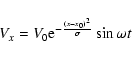
The tube is driven at one footpoint so that a kink wave is introduced into the tube. The tubes are vertical at the point of driving and the velocity perpendicular to the tube axis (Vx) is specified.
This boundary driving introduces kink oscillations into the loop which are in the plane of the loop equilibria. At the loop apex these oscillations are vertical, i.e. in the y direction and hence correspond to the oscillations observed in Wang & Solanki (2004). The more common situation in which loops oscillate out of the loop plane (Aschwanden et al. 1999) cannot be simulated in a 2D Cartesian code, and so are not considered here.
For most of the simulations, all boundaries except for the area which is driven, are line-tied. The driver specifies Vx as stated and line-ties all other quantities. For the lower boundary this is physically realistic representing the higher density of chromospheric material. Near the other boundaries velocity damping regions are introduced where the velocity obtained from the core solver is artificially reduced to simulate the effect of open boundaries. Tests in which these boundaries were moved further away reproduce the results presented here. Provided the damping region ramps up the damping on a length scale larger than the incoming MHD wave and only outward propagating waves, i.e. not standing wave structures, are present in the outer regions of the solution domain this approach leads to effective open boundary conditions.
For a kink mode of given ![]() and k the requirement
for the mode to be locally propagating at any point is
and k the requirement
for the mode to be locally propagating at any point is
Even with a uniform background density the magnetic field given by
Eq. (5) will yield an Alfvén speed profile which
decreases radially from the origin. The superimposed density maximum
of the tube leads to a local minimum in the Alfvén speed profile
at the loop centre, as can be seen in Fig. 2. If the three categories are considered
again, they are now found to have changed. Firstly, for the dashed line, there is now a finite
radius at which wave solutions exist and the wave would become propagating. For the dotted line,
the wave ceases to be freely propagating as the origin is approached. The most interesting
change is for the dot dashed line, which previously was interpreted as a trapped mode. Now the
mode is propagating in the tube body, not propagating in the region close to the tube, and
propagating again at larger radial distances from the tube. The barrier to waves leaving the tube
is now of finite thickness, where previously it was infinitely thick. It is therefore possible to
leak energy by tunneling through this barrier. The implication of this is that for this type of
curved tube there are no perfectly confined modes, only modes with varying degrees of leakage
through tunneling. The modes studied in this paper are all of the type corresponding to the dot dashed
line in Fig. 2 and thus would correspond to trapped modes in the straight tube.
For both Figs. 1 and 2 the same parameters were used,
![]() ,
but for the straight tube, the magnetic field
is assumed to be constant = 1 everywhere.
In Fig. 2 we have assumed that the local phase speed of the mode is independent
of distance from the tube axis.
However it is only
,
but for the straight tube, the magnetic field
is assumed to be constant = 1 everywhere.
In Fig. 2 we have assumed that the local phase speed of the mode is independent
of distance from the tube axis.
However it is only ![]() which is constant and k decreases with increasing radius due
to geometric effects. This merely decreases the region through which kink modes must tunnel and
therefore does not affect the argument. In this paper, the phrase "leaky mode'' is used to
refer to a mode which exhibits this loss due to tunneling.
which is constant and k decreases with increasing radius due
to geometric effects. This merely decreases the region through which kink modes must tunnel and
therefore does not affect the argument. In this paper, the phrase "leaky mode'' is used to
refer to a mode which exhibits this loss due to tunneling.
![\begin{figure}
\par\includegraphics[width=7.7cm,clip]{2527fig1.eps}
\end{figure}](/articles/aa/full/2005/29/aa2527-04/img48.gif) |
Figure 1:
Alfvén speed vs. distance from tube axis for straight tube. For values of
|
| Open with DEXTER | |
![\begin{figure}
\par\includegraphics[width=7.7cm,clip]{2527fig2.eps}
\end{figure}](/articles/aa/full/2005/29/aa2527-04/img49.gif) |
Figure 2: Alfvén speed vs. distance from tube axis for curved tube. The horizontal lines are plotted at the same points as in Fig. 1. |
| Open with DEXTER | |
The exact form of Fig. 2 is dependent upon the choice of magnetic field and density profile and hence the thickness of the barrier that the wave must tunnel through is related to these parameters. The most important feature is the radially decreasing Alfvén speed profile for the curved tube, and this is reproduced for any sensible choice of density profile, once a radially decreasing magnetic field is specified. However, it would be expected that the leakage rate would be related to this profile, and a detailed parameter study of such effects will be the subject of a later publication.
The quantity of interest for comparison with observational data in Wang & Solanki (2004) is the damping time of normal modes of a curved flux tube. Here we use a driver function at one footpoint to introduce waves of a desired wavelength into the flux tube. We therefore excite preferentially that mode which matches our driving frequency. We cannot simply start at t=0 with a kink mode imposed as we do not know the radial structure of the mode. By driving at one footpoint we can therefore excite a particular mode wavelength. There is no suggestion here that this is how such modes may be excited in reality and indeed for the fundamental mode observation suggest that this is excited by nearby flare activity. The driver is thus a convenient mechanism of initiating the normal mode. Once the kink oscillations are well established the footpoint driver is turned off. The final mode is therefore line-tied at both footpoints.
![\begin{figure}
\par\includegraphics[width=7.7cm,clip]{2527fig3.eps}
\end{figure}](/articles/aa/full/2005/29/aa2527-04/img50.gif) |
Figure 3:
Contours of
|
| Open with DEXTER | |
![\begin{figure}
\par\includegraphics[width=7.6cm,clip]{2527fig4.eps}
\end{figure}](/articles/aa/full/2005/29/aa2527-04/img51.gif) |
Figure 4:
Contours of
|
| Open with DEXTER | |
In all figures,
![]() is the velocity normal to the
local magnetic field, which is indicative of the fast kink wave
being considered. All physical parameters have the values given in
Sect. 2.
is the velocity normal to the
local magnetic field, which is indicative of the fast kink wave
being considered. All physical parameters have the values given in
Sect. 2.
While the driver is still active, the pattern of leakage, particularly for shorter wavelengths is
asymmetric, with greater loss rates above the driving point (see Fig. 3).
This implies that the driver is not
the perfect horizontal eigenmode of the curved flux tube , i.e. the horizontal profile of
the driver is not the correct profile for a mode of the tube. The
driver function could in principle be decomposed into trapped MHD eigenmodes, if these were known,
and freely propagating MHD wave sources. In these simulations the lowest harmonic trapped components
are established inside the tube while the remnant of the driving function which cannot be decomposed into
these modes acts as a source of propagating waves. The
driver periods were arbitrarily chosen, and as such are not the same
as the periods of the excited eigenmodes. Further simulations were
performed where the period of the driver was set to the period of the
observed eigenmode, but this caused no significant change in the
result. This asymmetry is not as
noticeable for longer
wavelengths, since the greater leakage due to curvature masks the leakage due to driver mismatch.
The longest wavelength which can clearly be excited by this boundary driving is shown in
Fig. 4. The mode structure can more clearly be seen in
![]() ,
which is shown in Fig. 5.
,
which is shown in Fig. 5.
Since the driver has the
wrong symmetry for the final mode there is always an asymmetric component which is also introduced
through this procedure. This can be clearly seen as a superimposed long period oscillation on ![]() ,
where
,
where
![]() and the integration is over the volume of the flux tube,
(see Fig. 6). This long period oscillation is due to an Alfvén pulse bouncing between the line-tied loop footpoints. The Alfvén
pulse is generated by the termination of driving. If the amplitude
of the driver is decreased over a longer time the amplitude of this
long period oscillation is reduced. However the period is unchanged as this is still the bounce time of an Alfvén pulse between the footpoints. Simulations show that the presence of this pulse in no
way affects the obtained decay rates. For this reason longer driver
ramp down times were not used, as this would require longer run
times to obtain the same free decay range. This does not affect the calculated
decay times of the symmetric mode. However, the excitation by footpoint driving does mean that
it is not possible to excite the longest wavelength mode with this
procedure. Another problem with the driving procedure is that unless
the driver frequency is a perfect match to an eigenfrequency of the
loop, the loop will in fact have a superposition of several eigenmodes, although it would be
expected that the greatest amplitude will be in the eigenmode with the frequency closest to
the driver.
and the integration is over the volume of the flux tube,
(see Fig. 6). This long period oscillation is due to an Alfvén pulse bouncing between the line-tied loop footpoints. The Alfvén
pulse is generated by the termination of driving. If the amplitude
of the driver is decreased over a longer time the amplitude of this
long period oscillation is reduced. However the period is unchanged as this is still the bounce time of an Alfvén pulse between the footpoints. Simulations show that the presence of this pulse in no
way affects the obtained decay rates. For this reason longer driver
ramp down times were not used, as this would require longer run
times to obtain the same free decay range. This does not affect the calculated
decay times of the symmetric mode. However, the excitation by footpoint driving does mean that
it is not possible to excite the longest wavelength mode with this
procedure. Another problem with the driving procedure is that unless
the driver frequency is a perfect match to an eigenfrequency of the
loop, the loop will in fact have a superposition of several eigenmodes, although it would be
expected that the greatest amplitude will be in the eigenmode with the frequency closest to
the driver.
![\begin{figure}
\par\includegraphics[width=7.7cm,clip]{2527fig5.eps}
\end{figure}](/articles/aa/full/2005/29/aa2527-04/img55.gif) |
Figure 5:
Contours of
|
| Open with DEXTER | |
![\begin{figure}
\par\includegraphics[width=8.6cm,clip]{2527fig6.eps}\end{figure}](/articles/aa/full/2005/29/aa2527-04/img56.gif) |
Figure 6:
The decay of |
| Open with DEXTER | |
![\begin{figure}
\par\includegraphics[width=7.7cm,clip]{2527fig7.eps}
\end{figure}](/articles/aa/full/2005/29/aa2527-04/img57.gif) |
Figure 7:
Contours of
|
| Open with DEXTER | |
![\begin{figure}
\par\includegraphics[width=8.4cm,clip]{2527fig8.eps}
\end{figure}](/articles/aa/full/2005/29/aa2527-04/img58.gif) |
Figure 8: Decay constant vs. observed eigenmode period in dimensionless units for domain with velocity damping boundaries and a density contrast ratio of 10. This is one of a family of similar curves for different density contrast ratios. |
| Open with DEXTER | |
In Fig. 7, which is after the driver has been turned off,
this asymmetry is gone, and the results show that the tube is radiating
symmetrically all along the tube. Although the presence of
the driver changes the symmetry of the system, the propagating waves
radiated by the tube have the same period and phase speed both during
driving and after driving has been terminated. After an initial transient period, the decay of
![]() settles
down into an exponential decay(
settles
down into an exponential decay(
![]() )
with a well defined
decay constant. The diagnostic used is the decay of
)
with a well defined
decay constant. The diagnostic used is the decay of
![]() where the integration is over the
region of the domain that is within w/2 (as defined in Eq. (6)), of the tube axis. When the
initial transient period has settled the decay constant is measured by fitting a straight line
to
where the integration is over the
region of the domain that is within w/2 (as defined in Eq. (6)), of the tube axis. When the
initial transient period has settled the decay constant is measured by fitting a straight line
to
![]() vs. time for a variety of driver periods
(Fig. 8). The driver periods were
vs. time for a variety of driver periods
(Fig. 8). The driver periods were
![]() .
The observed
periods of the eigenmodes are
.
The observed
periods of the eigenmodes are
![]() .
The error bars in
Fig. 8 are the 2
.
The error bars in
Fig. 8 are the 2![]() uncertainties on the fit of the straight line to
uncertainties on the fit of the straight line to
![]() vs. time.
vs. time.
Using ![]() as a diagnostic for the mode decay is
numerically convenient and provided most of the input energy is in a
single dominant mode will clearly give the correct decay
rate. However, a different diagnostic is used by Wang & Solanki
(2004), so for direct comparison with observations the
technique used in that paper is also used here for comparison. The
equivalence of the diagnostics can be confirmed directly by
analyzing one dataset using data from a slit at the loop apex. A
rectangular slit was positioned at the loop apex, with a width of
1/30th of the loop length and a height that was larger than the loop
radius. The motion of the centre of mass of the loop over time was
then measured, and a damped sine wave fit was made (see
Fig. 9). The resulting
as a diagnostic for the mode decay is
numerically convenient and provided most of the input energy is in a
single dominant mode will clearly give the correct decay
rate. However, a different diagnostic is used by Wang & Solanki
(2004), so for direct comparison with observations the
technique used in that paper is also used here for comparison. The
equivalence of the diagnostics can be confirmed directly by
analyzing one dataset using data from a slit at the loop apex. A
rectangular slit was positioned at the loop apex, with a width of
1/30th of the loop length and a height that was larger than the loop
radius. The motion of the centre of mass of the loop over time was
then measured, and a damped sine wave fit was made (see
Fig. 9). The resulting ![]() of
of
![]() equals the value obtained from the
previous approach which gave
equals the value obtained from the
previous approach which gave
![]() .
The measured period of the standing mode
oscillation is
.
The measured period of the standing mode
oscillation is
![]() ,
and is equal within error to the
other method used, which yields a period of
,
and is equal within error to the
other method used, which yields a period of
![]() .
The lower error estimates for
the calculations based on the decay of
.
The lower error estimates for
the calculations based on the decay of ![]() are due the average for
are due the average for ![]() using more
data points, i.e. more information.
using more
data points, i.e. more information.
The observed leaking waves are propagating at an angle to the field lines implying that they must be fast waves. To confirm this a plot of magnetic and gas pressures parallel to the y-axis was plotted outside the tube (see Fig. 10). Since the pressures are in phase this confirms that the wave is indeed a fast wave. The period of these fast waves is within 5% of the period of the eigenmode in the tube both while the system is being driven and after the driver is deactivated. The phase speed away from the tube bounadry is the local phase speed for a fast wave at that point
![\begin{figure}
\par\includegraphics[width=8.5cm,clip]{2527fig9.eps}
\end{figure}](/articles/aa/full/2005/29/aa2527-04/img70.gif) |
Figure 9: Fitting a damped sine wave to the observed oscillations of the loop apex. The symbols are the points obtained from the simulation, the solid line is the best fit damped sine wave. The damping time and period are both equivalent to those obtained from the main diagnostic. |
| Open with DEXTER | |
![\begin{figure}
\par\includegraphics[width=8.4cm,clip]{2527fg10.eps}
\end{figure}](/articles/aa/full/2005/29/aa2527-04/img71.gif) |
Figure 10: Plot of the magnetic (solid line) and thermal (dashed line) pressure perturbations along a straight line at x=0 between y=2 and the top of the simulation domain for the same simulation and at the same time as Fig. 7. |
| Open with DEXTER | |
The results show that the magnitude of the decay constant increases linearly with increasing
period. The linear fit is
![]() ,
where P is the period of the mode,
and
,
where P is the period of the mode,
and
![]() where
where ![]() is the decay time. Both of these times are still normalized
as given in Sect. 2. The maximum period which can successfully be excited by the footpoint
driving mechanism outlined above (approximately 1.54 in these normalized units) is the fifth
harmonic of the loop. To compare these results with observations we assume the linear fit
remains valid out to a period of 7.7, which corresponds to the fundamental mode, and
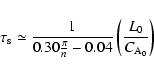
estimate the decay constant for this mode to be 1.1. Hence, these results suggest that for
our chosen equilibrium the ratio of decay time to period for the fundamental kink mode is 0.12.
is the decay time. Both of these times are still normalized
as given in Sect. 2. The maximum period which can successfully be excited by the footpoint
driving mechanism outlined above (approximately 1.54 in these normalized units) is the fifth
harmonic of the loop. To compare these results with observations we assume the linear fit
remains valid out to a period of 7.7, which corresponds to the fundamental mode, and
estimate the decay constant for this mode to be 1.1. Hence, these results suggest that for
our chosen equilibrium the ratio of decay time to period for the fundamental kink mode is 0.12.
To test the sensitivity of these results to choice of equilibrium the plasma ![]() ,
coronal loop
width and density contrast (ratio of maximum density inside tube to background density) were
varied. There is only a weak dependence on
,
coronal loop
width and density contrast (ratio of maximum density inside tube to background density) were
varied. There is only a weak dependence on ![]() with an increase in
with an increase in ![]() by a factor of 10
only increasing the decay rate by about 3%. Similarly reducing
by a factor of 10
only increasing the decay rate by about 3%. Similarly reducing ![]() by a factor of 10
reduced the decay rate by about 3%. Doubling the width of the coronal loop increased the decay rate
by 3% but decreasing the loop width had no detectable effect on the decay rate. The most critical
parameter from these test was the density contrast. Doubling the density contrast decreases the
decay rate by a factor of 1.5. In fact over a range of tests the scaling of decay rate with density
contrast suggest that the decay rate varies inversely with the square root of the density ratio
between the centre of the tube and the background value. All of the figures presented in this paper
are for a density contrast ratio of 10. The variation of decay rate with
by a factor of 10
reduced the decay rate by about 3%. Doubling the width of the coronal loop increased the decay rate
by 3% but decreasing the loop width had no detectable effect on the decay rate. The most critical
parameter from these test was the density contrast. Doubling the density contrast decreases the
decay rate by a factor of 1.5. In fact over a range of tests the scaling of decay rate with density
contrast suggest that the decay rate varies inversely with the square root of the density ratio
between the centre of the tube and the background value. All of the figures presented in this paper
are for a density contrast ratio of 10. The variation of decay rate with ![]() and
density contrast is consistent with the conclusions drawn in Smith et al. (1997). However,
Smith et al. (1997) did not quantify decay rates so further comparison is not possible.
The variation of decay rate with tube width derived here is the opposite as the trend inferred
from the eigenfunctions alone in Smith et al. (1997). Possible reasons for the discrepancies
between this paper and the results in Smith et al. (1997) will be discussed later.
and
density contrast is consistent with the conclusions drawn in Smith et al. (1997). However,
Smith et al. (1997) did not quantify decay rates so further comparison is not possible.
The variation of decay rate with tube width derived here is the opposite as the trend inferred
from the eigenfunctions alone in Smith et al. (1997). Possible reasons for the discrepancies
between this paper and the results in Smith et al. (1997) will be discussed later.
In this paper the decay of standing modes in curved flux tubes is considered in 2D Cartesian
co-ordinates by establishing a wave in the tube, by means of boundary driving at the footpoint,
and then allowing the tube to relax to a normal mode structure. The decay constant of these
normal modes is found to vary linearly with the period of the excited mode, with longer
driving periods (longer wavelengths) decaying more rapidly. This result is in contrast to that
of Smith et al. (1997), where it was concluded that longer wavelengths decay less quickly.
It should be noted that both this paper and the Smith et al. paper imply higher harmonic
standing mode when talking about shorter wavelength. The normalization used in this code means
that a wave of the same harmonic number in a longer tube, although having a longer wavelength,
would decay more slowly. This can be seen by writing the normalized result
![]() as
as
![]() ,
converting to real units, and assuming a semi circular loop to give
,
converting to real units, and assuming a semi circular loop to give
 |
(9) |
| (10) |
![\begin{figure}
\par\includegraphics[width=7.5cm,clip]{2527fg11.eps}
\end{figure}](/articles/aa/full/2005/29/aa2527-04/img82.gif) |
Figure 11:
Pattern of
|
| Open with DEXTER | |
In Wang & Solanki (2004), the observed kink oscillation had a period of 234 s and a decay time of 714 s. Hence the observations for this loop give a ratio of decay time to mode period for the fundamental mode of 3.05. In this paper we have chosen an equilibrium and excited modes which would be trapped in a straight tube. However, these modes become leaky in loop geometry and the calculated ratio of decay time to mode period for this equilibrium is 0.12. This value is smaller than that observed in Wang & Solanki (2004), but it is possible to increase the damping time by choosing an equilibrium such that the tunneling distance is greater. Also, although the linear fit to the data points given here is good, there is a priori no reason to assume that this linear fit remains valid out to the fundamental mode. Also the inclusion of gravity may decrease the decay rate observed here, and further work is necessary to elucidate the exact effects of gravity on the decay rate. Despite these limitations of the current approach it does seems highly likely that the observed damping of kink oscillations, when the oscillations are in the plane of the equilibrium loop, can be entirely accounted for by wave leakage. There are two cautionary points which must however be emphasized. Firstly the decay time for the fundamental mode calculated in this paper is based on an extrapolation from higher harmonics. The fifth harmonic was the longest wavelength directly simulated and reported in this paper. Secondly, without detailed knowledge of the internal structure of the observed loop, e.g. its density contrast, it is not possible to show that wave leakage through tunneling is the dominant loss mechanism.
In conclusion, these results show that even in the absence of anomalously large viscosity or magnetic diffusivity it is possible to obtain decay rates for vertically polarized kink waves in coronal flux tubes that are on the order of the decay rates observed by imaging telescopes. The results presented here give decay rates that are faster than those observed in the corona, but including gravity would decrease the rate of decrease of Alfvén speed with height, increasing the thickness of the tunneling layer, and hence the decay time. Also simply increased the density contrast reduces the decay rate. The important point is that the theory of wave tunneling can easily get decay rates consistent with observations. This effect is purely due to the change of system geometry to include loop curvature. The loss of energy from the flux tubes is in the form of propagating fast magneto-acoustic waves which are effectively unobservable. These results apply only to kink oscillations in the plane of the loop equilibrium and whether wave leakage due to tunneling plays a significant role in damping kink oscillations which are out of the equilibrium plane remains an open question.