A&A 438, 571-583 (2005)
DOI: 10.1051/0004-6361:20034189
Proper motion of H2O masers in IRAS 20050+2720 MMS1: an AU scale jet associated with an intermediate-mass class 0 source
R. S. Furuya1 -
Y. Kitamura2 -
A. Wootten3 - M. J. Claussen4 - R. Kawabe5
1 - Division of Physics, Mathematics, and Astronomy, California Institute of Technology,
MS 105-24, 1201 East California Boulevard, Pasadena, CA 91125, USA
2 -
Institute of Space and Astronautical Science,
Japan Aerospace Exploration Agency,
Yoshinodai 3-1-1, Sagamihara, Kanagawa 229-8510, Japan
3 -
National Radio Astronomy Observatory,
520 Edgemont Road, Charlottesville, VA 22903, USA
4 -
National Radio Astronomy Observatory,
1003 Lopezville Road, Socorro, NM 87801, USA
5 -
National Astronomical Observatory,
Osawa 2-21-1, Mitaka, Tokyo 181-8588, Japan
Received 13 August 2003 / Accepted 26 March 2005
Abstract
We conducted a 4 epoch, 3 month, VLBA proper motion study
of H2O masers toward an intermediate-mass class 0 source IRAS 20050+2720 MMS1
(d=700 pc).
The region of IRAS 20050+2720 contains at least 3 bright young stellar objects
at millimeter to
submillimeter wavelengths and shows three pairs of CO outflow lobes:
the brightest source MMS1,
which shows an extremely high velocity (EHV) wing emission,
is believed to drive the outflow(s).
From milli-arcsecond (mas) resolution VLBA images,
we found two groups of H2O maser spots
at the center of the submillimeter core of MMS1.
One group consists of more than  50 intense maser spots;
the other group consisting of several weaker maser spots
is located at 18 AU south-west of the intense group.
Distribution of the maser spots in the intense group shows an arc-shaped structure
which includes the maser spots that showed a clear velocity gradient.
The spatial and velocity structures of the maser spots in the arc-shape
did not significantly change through the 4 epochs.
Furthermore, we found a relative proper motion between the two groups.
Their projected separation increased by
50 intense maser spots;
the other group consisting of several weaker maser spots
is located at 18 AU south-west of the intense group.
Distribution of the maser spots in the intense group shows an arc-shaped structure
which includes the maser spots that showed a clear velocity gradient.
The spatial and velocity structures of the maser spots in the arc-shape
did not significantly change through the 4 epochs.
Furthermore, we found a relative proper motion between the two groups.
Their projected separation increased by
 mas over the 4 epochs
along a line connecting them
(corresponding to a transverse velocity of 14.4 km s-1).
The spatial and velocity structures of the intense group and the
relative proper motions strongly suggest that the maser emission is
associated with a protostellar jet.
Comparing the observed LSR velocities with calculated radial velocities
from a simple biconical jet model, we conclude that the most of the maser
emission is likely to be associated with an accelerating biconical jet
that has large opening angle of about
mas over the 4 epochs
along a line connecting them
(corresponding to a transverse velocity of 14.4 km s-1).
The spatial and velocity structures of the intense group and the
relative proper motions strongly suggest that the maser emission is
associated with a protostellar jet.
Comparing the observed LSR velocities with calculated radial velocities
from a simple biconical jet model, we conclude that the most of the maser
emission is likely to be associated with an accelerating biconical jet
that has large opening angle of about
 .
The large opening angle of the jet traced by the masers would support
the hypothesis that poor jet collimation is
an inherent property of luminous (proto)stars.
.
The large opening angle of the jet traced by the masers would support
the hypothesis that poor jet collimation is
an inherent property of luminous (proto)stars.
Key words: stars: formation -
radio lines: ISM -
ISM: jets and outflows -
ISM: individual objects: IRAS 20050+2720 MMS1
1 Introduction
Water maser surveys using single-dish radio telescopes toward
intermediate- and low-mass young stellar objects (YSOs) have been extensively performed
since the early 1990s (e.g., Claussen et al. 1996).
From a multi-epoch survey toward low-mass YSOs
(bolometric luminosity,
 ),
Furuya et al. (2001, 2003)
found that class 0 objects are favored sites for the masers:
the detection rates are derived to be 40% for class 0, while only
),
Furuya et al. (2001, 2003)
found that class 0 objects are favored sites for the masers:
the detection rates are derived to be 40% for class 0, while only
 for class I.
It is known that the isotropic maser luminosity,
for class I.
It is known that the isotropic maser luminosity,
 ,
correlates well with
the bolometric luminosity of the source
(Wilking et al. 1994; Furuya et al. 2001).
However, it is interesting to note that the presence of the maser emission is strictly
related to that of high-velocity outflowing gas in the case of
high-mass YSOs (Felli et al. 1992).
Furuya et al. (2001) showed that the H2O maser luminosity in low-mass
stars is more closely related to the luminosity of 100 AU
scale radio jets rather than the mechanical luminosity of larger scale
CO outflows. In fact, VLA observations have revealed that
the masers tend to be distributed within several hundred AU of the central
stars (e.g., Wootten 1989).
Although some H2O masers are reported to be associated with protostellar disks
(e.g., Fiebig et al. 1996; Torrelles et al. 1998; Seth et al. 2002),
high resolution VLBI observations have demonstrated
the presence of knots and shock structures
which are reminiscent of those of ionized jets in the larger scale
Harbig Haro objects, suggesting that in most cases the masers originate
in shocks produced by jets from protostars
(e.g., Claussen et al. 1998; Furuya et al. 2000).
There are a few published VLBI water maser studies of the jets and outflows from
intermediate-mass young stellar objects (Patel et al. 2000; Seth et al. 2002).
In order to extend our knowledge of H2O masers in
intermediate-mass YSOs, we have conducted multi-epoch VLBA observations
of H2O masers towards the intermediate-mass YSO IRAS 20050+2720
(d=700 pc).
,
correlates well with
the bolometric luminosity of the source
(Wilking et al. 1994; Furuya et al. 2001).
However, it is interesting to note that the presence of the maser emission is strictly
related to that of high-velocity outflowing gas in the case of
high-mass YSOs (Felli et al. 1992).
Furuya et al. (2001) showed that the H2O maser luminosity in low-mass
stars is more closely related to the luminosity of 100 AU
scale radio jets rather than the mechanical luminosity of larger scale
CO outflows. In fact, VLA observations have revealed that
the masers tend to be distributed within several hundred AU of the central
stars (e.g., Wootten 1989).
Although some H2O masers are reported to be associated with protostellar disks
(e.g., Fiebig et al. 1996; Torrelles et al. 1998; Seth et al. 2002),
high resolution VLBI observations have demonstrated
the presence of knots and shock structures
which are reminiscent of those of ionized jets in the larger scale
Harbig Haro objects, suggesting that in most cases the masers originate
in shocks produced by jets from protostars
(e.g., Claussen et al. 1998; Furuya et al. 2000).
There are a few published VLBI water maser studies of the jets and outflows from
intermediate-mass young stellar objects (Patel et al. 2000; Seth et al. 2002).
In order to extend our knowledge of H2O masers in
intermediate-mass YSOs, we have conducted multi-epoch VLBA observations
of H2O masers towards the intermediate-mass YSO IRAS 20050+2720
(d=700 pc).
2 IRAS 20050+2720
IRAS 20050+2720 is surrounded by a large cluster of
low-mass stars
(Chen et al. 1997; Wilking et al. 1989)
and has a luminosity in the IRAS bands of
 (Molinari et al. 1996).
The IRAS source has been categorized as a luminous
class 0 protostar in the early compilation (Bachiller 1996).
Recent SCUBA imaging (Chini et al. 2001) revealed the presence of a bright central object
(IRAS 20050+2720 MMS1) and two associated objects located 2' south-east.
The brightest source MMS1 is identified as the IRAS source.
Although IRAS 20050+2720 was not categorized as class 0 in the updated
compilation (Andr
(Molinari et al. 1996).
The IRAS source has been categorized as a luminous
class 0 protostar in the early compilation (Bachiller 1996).
Recent SCUBA imaging (Chini et al. 2001) revealed the presence of a bright central object
(IRAS 20050+2720 MMS1) and two associated objects located 2' south-east.
The brightest source MMS1 is identified as the IRAS source.
Although IRAS 20050+2720 was not categorized as class 0 in the updated
compilation (Andr
 et al. 2000),
Chini et al. (2001) reported that the source MMS1 is very likely to be at the class 0 stage.
This is because MMS1 shows a ratio of FIR luminosity (
et al. 2000),
Chini et al. (2001) reported that the source MMS1 is very likely to be at the class 0 stage.
This is because MMS1 shows a ratio of FIR luminosity (
 )
and
submillimeter luminosity (
)
and
submillimeter luminosity (
 )
for
)
for
 m of
164
which satisfies one of the definitions of class 0
(Andr
et al. 1993;
m of
164
which satisfies one of the definitions of class 0
(Andr
et al. 1993;
 ).
).
Bachiller et al. (1995; hereafter BFT95)
found three pairs of outflow lobes emanating from
the vicinity of the source MMS1 from the
IRAM 30-m telescope CO J=2-1 observations.
One of the lobe pairs is a highly collimated jet with
extremely high velocity (EHV) emission whose terminal velocity
exceeds 60 km s-1 with respect to the ambient cloud velocity.
The presence of the EHV outflow suggests that the driving source of the EHV outflow
is in its most powerful outflow phase.
BFT95 suggested that two or three independent outflows emanate from
different YSOs embedded in the cloud core,
although the driving sources have not been identified.
H2O maser emission in the IRAS 20050+2720 region was first detected by
Palla et al. (1991),
and was subsequently observed by the Arcetri group
(Brand et al. 1994;
Palumbo et al. 1994):
all of the detected emission was seen around the cloud velocity
(
 km s-1).
Using the Nobeyama 45-m telescope, Furuya et al. (2003)
detected EHV maser emission at
km s-1).
Using the Nobeyama 45-m telescope, Furuya et al. (2003)
detected EHV maser emission at
 km s-1.
The EHV emission was blueshifted with respect to the cloud velocity,
while no high velocity emission was detected on the redshifted side.
This source also showed weak, blueshifted, intermediate high velocity
(IHV) components
at
km s-1.
The EHV emission was blueshifted with respect to the cloud velocity,
while no high velocity emission was detected on the redshifted side.
This source also showed weak, blueshifted, intermediate high velocity
(IHV) components
at
 and
and
 in 1998 February.
In 1999, we carried out VLA observations and
found that all of the maser emission was located within 5''
(350 AU) from the source MMS1.
Our VLA observations revealed that
the EHV emission is located exactly at the JCMT position for source MMS1,
while the low-velocity components around the cloud velocity are located to
in 1998 February.
In 1999, we carried out VLA observations and
found that all of the maser emission was located within 5''
(350 AU) from the source MMS1.
Our VLA observations revealed that
the EHV emission is located exactly at the JCMT position for source MMS1,
while the low-velocity components around the cloud velocity are located to
 west and
 north of the
EHV emission (Furuya et al. 2003).
Suspecting multiplicity of CO outflows and the fact that the SCUBA beam
(8.3'' at 450
north of the
EHV emission (Furuya et al. 2003).
Suspecting multiplicity of CO outflows and the fact that the SCUBA beam
(8.3'' at 450  m; Chini et al. 2001) is larger
than the separation of the two maser components,
we made high resolution continuum images of the region with the OVRO mm-array.
In order to investigate the detailed structure of the masers,
we carried out extremely high angular resolution VLBA observations.
m; Chini et al. 2001) is larger
than the separation of the two maser components,
we made high resolution continuum images of the region with the OVRO mm-array.
In order to investigate the detailed structure of the masers,
we carried out extremely high angular resolution VLBA observations.
3 Observations
Aperture synthesis observations of continuum emission at 3 mm were
carried out using the six-element Owens Valley Radio Observatory (OVRO)
Millimeter Array from 2002 December to 2003 February with the H and E array configurations.
The phase tracking center was
 (J2000) = 20
 07
07 5
5
 87,
87,
 (J2000) = 27
 28
28 59
80.
The field of view (FOV) was 65
59
80.
The field of view (FOV) was 65
 .
All of the element antennas are equipped with SIS receivers having system noise
temperatures in double-sideband of 200 K toward the zenith at 93 GHz.
We tuned the 3 mm SIS receiver at the frequencies of N2H+ (1-0) line
(93.173 GHz) for the upper sideband and
H13CO+ (1-0) line (86.754 GHz) for the lower side band.
A detailed presentation of the results of the molecular line emission will be
published elsewhere (Furuya et al., in preparation).
The Continuum Correlator was configured for both the
sidebands, with a total bandwidth of 3 GHz.
We used 3C 454.3 and 3C 84 as a passband calibrator and J2025+337
as a phase and gain calibrator.
Flux density of J2025+337 was measured by comparison to that of Uranus:
it was stable in the range
from 1.2 to 1.5 Jy during the observation period.
The overall flux uncertainty is about 20%.
The data calibration was done using originally developed software at OVRO,
and the image construction was performed using the AIPS package of the NRAO.
After merging the data in both the sidebands,
we constructed continuum emission images
with two beam weightings.
Synthesized beam sizes were
.
All of the element antennas are equipped with SIS receivers having system noise
temperatures in double-sideband of 200 K toward the zenith at 93 GHz.
We tuned the 3 mm SIS receiver at the frequencies of N2H+ (1-0) line
(93.173 GHz) for the upper sideband and
H13CO+ (1-0) line (86.754 GHz) for the lower side band.
A detailed presentation of the results of the molecular line emission will be
published elsewhere (Furuya et al., in preparation).
The Continuum Correlator was configured for both the
sidebands, with a total bandwidth of 3 GHz.
We used 3C 454.3 and 3C 84 as a passband calibrator and J2025+337
as a phase and gain calibrator.
Flux density of J2025+337 was measured by comparison to that of Uranus:
it was stable in the range
from 1.2 to 1.5 Jy during the observation period.
The overall flux uncertainty is about 20%.
The data calibration was done using originally developed software at OVRO,
and the image construction was performed using the AIPS package of the NRAO.
After merging the data in both the sidebands,
we constructed continuum emission images
with two beam weightings.
Synthesized beam sizes were
 with natural weighting and
 with uniform weighting.
The 1
with uniform weighting.
The 1 rms noise levels for the continuum emission maps were
0.78 mJy beam-1 for the former and 1.5 mJy beam-1 for the latter.
rms noise levels for the continuum emission maps were
0.78 mJy beam-1 for the former and 1.5 mJy beam-1 for the latter.
![\begin{figure}
\par\includegraphics[angle=-90,width=15cm,clip]{0189fig1.ps} \end{figure}](/articles/aa/full/2005/29/aa0189-03/Timg42.gif) |
Figure 1:
Continuum emission maps taken with the OVRO millimeter array
toward IRAS 20050+2720 MMS1 with
a) natural weighting ( left) and b) uniform weighting ( right).
The solid contours start at  level with
interval and
the dashed contours are
level with
interval and
the dashed contours are  intervals started at
level.
The image noise levels are
0.78 and 1.5 mJy beam-1 for the panels a) and b), respectively.
The white dot and the eastern cross indicate the positions of the low-velocity and EHV
H2O maser emission (see Sect. 4.2.2).
The sizes of the synthesized beams are presented in the bottom right corners.
intervals started at
level.
The image noise levels are
0.78 and 1.5 mJy beam-1 for the panels a) and b), respectively.
The white dot and the eastern cross indicate the positions of the low-velocity and EHV
H2O maser emission (see Sect. 4.2.2).
The sizes of the synthesized beams are presented in the bottom right corners.
|
| Open with DEXTER |
VLBI observations of the H2O maser emission in IRAS 20050+2720 MMS1
were carried out using all 10 antennae of the Very Long Baseline Array (VLBA) of the
NRAO![[*]](/icons/foot_motif.gif) on 1999 April 1, May 5, June 5, and July 4
(hereafter epochs I, II, III and IV, respectively).
For epoch II, however, we could not use the antenna at North Liberty.
All of the data were obtained for 8-h integration each epoch.
We used a frequency setup of the 8 MHz IF bandwidth mode with 512 channels,
which provides a velocity resolution of 0.2 km s-1 at 22.235077 GHz.
This frequency setup covers the range of
on 1999 April 1, May 5, June 5, and July 4
(hereafter epochs I, II, III and IV, respectively).
For epoch II, however, we could not use the antenna at North Liberty.
All of the data were obtained for 8-h integration each epoch.
We used a frequency setup of the 8 MHz IF bandwidth mode with 512 channels,
which provides a velocity resolution of 0.2 km s-1 at 22.235077 GHz.
This frequency setup covers the range of
 to
+10.5 km s-1: this velocity coverage is sufficient to detect all of the
maser emission previously detected.
to
+10.5 km s-1: this velocity coverage is sufficient to detect all of the
maser emission previously detected.
The data were correlated at the NRAO Array Operation Center (Socorro, New Mexico).
We adopted a correlator averaging time of 2.16 s to
obtain 0.8'' radius FOV for the baseline of 4000 km.
Data calibration and image construction were performed using the AIPS package developed by the NRAO.
We used two bright quasars 3C 345 and 3C 454.3 to determine delay
and fringe rates as well as to calibrate bandpass response.
In the next section, we present the image construction,
identification of the maser emission
and further analysis together with the results.
4.1 Relation between millimeter continuum emission and masers
Figure 1 presents the OVRO continuum emission
maps together with the positions of the H2O masers.
There is a distinct continuum emission peak toward
the low-velocity and EHV maser emission.
To plot the absolute position of the low-velocity masers,
we adopted the results from the VLA measurements by Furuya et al. (2003)
and used the position offset of the EHV emission
obtained in Sect. 4.2.2.
Clearly the millimeter continuum emission is associated with
the low-velocity maser emission.
The peak of the continuum
emission is slightly shifted with respect to the maser emission.
We believe that this positional shift is real considering the baseline accuracies of
VLA and OVRO array
and angular separations between the calibrators and the source.
It is noteworthy that the continuum emission in the
natural weighting map (Fig. 1a)
is elongated to the east, namely, toward the EHV emission.
In the uniform weighting map (Fig. 1b),
one may notice that there is a
weak emission peak close to the EHV maser emission:
this fact might suggest that there are at least two YSOs in this region.
Table 1:
Summary of VLBA H2O maser observations.
We estimate molecular hydrogen mass (
 )
of the
core from the total flux density (
)
of the
core from the total flux density ( )
of the continuum emission
assuming that the emission is thermal radiation from dust grains.
We used a relation
)
of the continuum emission
assuming that the emission is thermal radiation from dust grains.
We used a relation
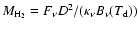 where
where
 is the mass opacity coefficient of the dust,
 is the dust temperature and
 is the Planck function.
The value of
at 3 mm is calculated with the
usual form of
is the Planck function.
The value of
at 3 mm is calculated with the
usual form of
 .
In order to keep consistency with the previous JCMT measurements by Chini et al. (2001),
we used the same
.
In order to keep consistency with the previous JCMT measurements by Chini et al. (2001),
we used the same  of 0.003 cm2 g-1 at 231 GHz,
 of 1.4, and
of 34 K.
We obtained
of 0.007
of 1.4, and
of 34 K.
We obtained
of 0.007  for
for
 mJy
by integrating the emission inside the 3
contour.
Note that the derived mass is a lower limit because interferometric
observations do not receive the whole flux from a source
due to the lack of short spatial frequency data.
In fact, the resultant projected baseline length of our OVRO observations
ranged from 6.2 to 75 k
mJy
by integrating the emission inside the 3
contour.
Note that the derived mass is a lower limit because interferometric
observations do not receive the whole flux from a source
due to the lack of short spatial frequency data.
In fact, the resultant projected baseline length of our OVRO observations
ranged from 6.2 to 75 k ,
which will
miss 50% of the flux from structures extending more than
16'' (0.05 pc at d=700 pc) (see Wilner & Welch 1994).
,
which will
miss 50% of the flux from structures extending more than
16'' (0.05 pc at d=700 pc) (see Wilner & Welch 1994).
In the following, we present results and analyses from the VLBA
observations of the H2O masers.
First, we carried out fringe-frequency analysis
(e.g., Walker 1981; Walker et al. 1982)
to cover a large FOV of 3'' which is 3 orders of magnitude
larger than the VLBA fringe-spacings.
The purpose of the fringe-frequency analysis was to search for
maser spots which were not excited during the VLA observations in 1999 February
(Furuya et al. 2003).
As expected from the VLA observations, we confirmed that
the distribution of the low-velocity masers is sufficiently compact to
perform standard Fourier synthesis.
The EHV emission was too weak to be detected with the fringe-frequency analysis.
Subsequently, we performed self-calibration using a
strong (45 Jy measured by Furuya et al. 2003) and
point-like maser spot identified at
 km s-1 as a model.
In the self-calibration procedure, we solved the time variation of the
complex gain for phase weighted by amplitude.
km s-1 as a model.
In the self-calibration procedure, we solved the time variation of the
complex gain for phase weighted by amplitude.
Applying the solutions from the self-calibration procedure,
we carried out image construction toward the low-velocity
emission (hereafter we refer to it as the MAIN Field):
the image area has 0.23'' size divided into 9 fields each of which
is of 77 milli-arcsecond (mas) size and
 pixels with a cell size of 0.15 mas.
We believe that the area size of 0.23'' was sufficient to search for
maser emission considering the absolute position accuracy of
the VLA observations (Sect. 2).
Subsequent to this coarse search,
we constructed a final image of 41 mas size for the area
where the low-velocity emission was detected,
with a smaller cell size of 0.08 mas.
The image noise level per velocity channel was typically 3 mJy beam-1
and the synthesized beam size was typically 1.0
pixels with a cell size of 0.15 mas.
We believe that the area size of 0.23'' was sufficient to search for
maser emission considering the absolute position accuracy of
the VLA observations (Sect. 2).
Subsequent to this coarse search,
we constructed a final image of 41 mas size for the area
where the low-velocity emission was detected,
with a smaller cell size of 0.08 mas.
The image noise level per velocity channel was typically 3 mJy beam-1
and the synthesized beam size was typically 1.0 0.5 mas
(Table 1).
0.5 mas
(Table 1).
![\begin{figure}
\par\includegraphics[angle=-90,width=8.6cm,clip]{0189fig2.eps} \end{figure}](/articles/aa/full/2005/29/aa0189-03/Timg60.gif) |
Figure 2:
Total integrated intensity map of the H2O masers in the MAIN Field of
IRAS 20050+2720 MMS1 obtained at the 3rd epoch (1999 June 5) of the VLBA observations.
Contour levels are 10, 20, 30, 50, 100, 200, 400, 800, 1600, 3200, 6400,
12 800 and 25 600 times the image noise level of
12.3 mJy beam-1 km s-1.
The inserted panel in the top right corner shows the H2O maser spectrum
obtained by integrating the emission over the presented region.
The vertical arrow shows the ambient cloud velocity (
 )
of )
of
 km s-1 estimated from
CS J=3-2 line observations (BFT95).
The size of the synthesized beam is presented in the bottom right corner. km s-1 estimated from
CS J=3-2 line observations (BFT95).
The size of the synthesized beam is presented in the bottom right corner.
|
| Open with DEXTER |
In Fig. 2, we show a total integrated intensity map of the MAIN Field,
namely low-velocity H2O masers, obtained in the Epoch III,
in which we attained the highest sensitivity among the 4 epochs.
The inserted panel presents the spectrum of the maser emission detected
in the region.
The overall distribution of the masers was similar for all 4 epochs:
we see bright maser emission peaks
at the field center (hereafter MAIN group) and an isolated emission peak
at 25 mas (corresponding to 18 AU)
south-west of the MAIN group.
Hereafter we call the latter emission the "SW feature'' instead of
"SW group'' because the emission showed a point-like structure.
The definition of "feature'' will be given in Sect. 4.3.
4.2.2 Extremely high velocity emission
In addition, we searched for the EHV emission on the basis of the snapshot
VLA D-array observations in 1999 February (Furuya et al. 2003)
and 2003 January (Claussen, private communication):
the former observations (hereafter Sub-Field 1) showed that the
 km s-1 emission is shifted by
 in RA and
 in Dec with respect to the low-velocity emission and
the latter observations (hereafter Sub-Field 2) showed that
the
in Dec with respect to the low-velocity emission and
the latter observations (hereafter Sub-Field 2) showed that
the
 and -78 km s-1 emission is shifted by
 in RA and
 in Dec.
Since these positions are outside the FOV correlated with the 1.6 km s-1 emission,
we used UV data only from
south-western 5 antennas (Fort Davis, Los Alamos, Pie Town, Kitt Peak and Owens Valley)
which provide a maximum spatial frequency of
in Dec.
Since these positions are outside the FOV correlated with the 1.6 km s-1 emission,
we used UV data only from
south-western 5 antennas (Fort Davis, Los Alamos, Pie Town, Kitt Peak and Owens Valley)
which provide a maximum spatial frequency of
 .
The synthesized beam sizes were typically
.
The synthesized beam sizes were typically
 mas and
the image noise levels per velocity channel were typically 5 mJy beam-1
(Table 1).
Applying the solution from the self-calibration procedure above,
we constructed images toward both the Sub-Fields.
mas and
the image noise levels per velocity channel were typically 5 mJy beam-1
(Table 1).
Applying the solution from the self-calibration procedure above,
we constructed images toward both the Sub-Fields.
We detected the maser emission peaking of
km s-1
in Sub-Field 2 where the
and -78 km s-1 emission
was detected with the VLA in 2003 January.
However, we did not see any maser emission around
and -78 km s-1 toward the two Sub-Fields.
The detected -93 km s-1 emission shows a point-like structure
located at 4184 mas east and 709 mas
south with respect to the
 km s-1
emission peak with which we performed the self-calibration.
km s-1
emission peak with which we performed the self-calibration.
![\begin{figure}
\par\includegraphics[angle=-90,width=17cm,clip]{0189fig3.eps} \end{figure}](/articles/aa/full/2005/29/aa0189-03/Timg69.gif) |
Figure 3:
Total integrated intensity maps (contours) overlaid with isovelocity maps
(images) for the MAIN Field of the H2O masers inIRAS 20050+2720.
The contour levels are the same as those in Fig. 2.
The velocity range shown here is from
 to 8.5 km s-1.
The white dots present peak positions of the maser spots.
Boxes with labels indicate identified maser features.
to 8.5 km s-1.
The white dots present peak positions of the maser spots.
Boxes with labels indicate identified maser features.
|
| Open with DEXTER |
4.3 Identification of maser spots and features
To identify maser "spots'' from the image,
we fitted a two-dimensional elliptical Gaussian profile
to individual possible spots.
We adopted a detection threshold of a signal-to-noise ratio
(S/N) larger than 10.
In this way, we detected  maser spots at each epoch
(Fig. 3).
We estimated the relative positional error for each spot (
maser spots at each epoch
(Fig. 3).
We estimated the relative positional error for each spot (
 )
to be
)
to be
 0.02 mas: the relative positional error of a point-like source convolved
with a Gaussian shaped beam is given by the relation of
0.02 mas: the relative positional error of a point-like source convolved
with a Gaussian shaped beam is given by the relation of
![$\sigma=0.45~\theta_{\rm syn}/[{S/N}]$](/articles/aa/full/2005/29/aa0189-03/img73.gif) (Condon 1997) where
(Condon 1997) where
 is the FWHM of the synthesized beam
(
is the FWHM of the synthesized beam
(
![$\theta_{\rm syn}=[\theta_{\rm maj}\times\theta_{\rm min}]^{1/2}$](/articles/aa/full/2005/29/aa0189-03/img75.gif) ).
).
Subsequent to the identification of the maser "spots'',
we divided them into groups, i.e.,
spatially localized "features'' with distinct peaks in line profiles:
we grouped the spots in adjacent velocity channels
that are distributed within one synthesized beam width.
Each feature is considered probably to represent a distinct clump of gas.
In Fig. 3,
only Features 4, 5, 9 and 13 showed emission
over the 4 epochs among the 14 features identified in the MAIN-Field.
Feature 2 persisted from Epoch I to III,
but disappeared in Epoch IV.
The other 9 features did not persist continuously more than 3 epochs.
Therefore, we do not consider these 9 features in our further analysis
of proper motion measurements.
For each feature, we calculated
an intensity-weighted mean position of the contributing maser spots:
its uncertainty is given by
![$\sigma_{\rm feature}=[\sum_{\rm spot} \sigma_{\rm spot}^2]^{1/2}$](/articles/aa/full/2005/29/aa0189-03/img76.gif) .
As summarized in Table 2, the resultant positional errors were
a few 0.01 mas for the 6 features in the MAIN-Field and
a few 0.1 mas for the EHV feature in the Sub-Field.
.
As summarized in Table 2, the resultant positional errors were
a few 0.01 mas for the 6 features in the MAIN-Field and
a few 0.1 mas for the EHV feature in the Sub-Field.
There is a velocity gradient of approximately 9 km s-1 over 10 mas
from Features 1 to 9.
Table 2:
Relative positions of the identified H2O maser features.
4.4 Spectra of the features and their time variation
For each maser feature identified, we obtained a spectrum
by integrating the intensity over the corresponding region.
Figure 4 represents spectra of the features
listed in Table 2.
Among the series of the 7 spectra, Features 2, 5 and EHV showed single-peaked
spectra while Features 4, 9, 13 and SW displayed multi-peaked spectra.
Using these spectra, we evaluated intensity-weighted mean velocities
(
 ;
Table 3).
The former single-peaked features did not show any prominent
trend of LSR-velocity change over the 4 epochs.
On the other hand,
the latter multiple-peaked features displayed small drifts.
We discuss the velocity drifts when we assess proper motions
of the features in the next subsection.
;
Table 3).
The former single-peaked features did not show any prominent
trend of LSR-velocity change over the 4 epochs.
On the other hand,
the latter multiple-peaked features displayed small drifts.
We discuss the velocity drifts when we assess proper motions
of the features in the next subsection.
4.5 Proper motions
Since VLBI observations generally do not provide absolute positions,
we adopt the brightest spot at
km s-1 in Feature 5
as a reference to examine the cross-epoch positional shifts of the maser features.
The selection of the 1.6 km s-1 spot is justified because
this spot does not show any velocity drift over the 4 epochs.
In addition, the spot is enough small to be used as a position reference
as shown in the following.
The correlated flux (i.e., fringe amplitude)
of the spot drops by a factor of 2 at a projected baseline length
of
 which corresponds to a fringe spacing of 0.06 mas.
This means that FWHM of the maser spot would be 0.06 mas
assuming that the spot has a Gaussian shape brightness distribution.
Note that the reference spot is not a complete point source compared with the
relative position accuracy of the features (Table 2).
Therefore, the size of the reference spot will be treated as a
positional uncertainty in our analyses.
which corresponds to a fringe spacing of 0.06 mas.
This means that FWHM of the maser spot would be 0.06 mas
assuming that the spot has a Gaussian shape brightness distribution.
Note that the reference spot is not a complete point source compared with the
relative position accuracy of the features (Table 2).
Therefore, the size of the reference spot will be treated as a
positional uncertainty in our analyses.
Table 3:
Mean LSR-velocitiesa (
)
for the identified maser features.
In Fig. 5, we present an overlay of the peak positions of
the maser spots together with boxes indicating the identified features.
The overall distribution of the maser spots does not change over
the 4 epochs: it shows an arc-shaped structure.
In Fig. 6, we present magnified overlays of the
7 features together with the intensity-weighted mean positions for the observing epochs
(Table 2).
As expected from Fig. 5,
most of the maser features in the MAIN Group do not show any prominent
positional shifts.
On the other hand,
Features SW and EHV displayed distinct positional shifts
as can be seen in Fig. 6:
the member spots of SW sequentially appeared from NE to SW
over the 4 epochs and those of EHV appeared from SE to NW.
These facts strongly suggest that the observed position shifts are caused
by real motions of the spatially localized masing gas.
In contrast, Features 2, 4 and 5 show neither well-defined
position shifts of member spots nor systematic motions of their
intensity-weighted mean positions.
![\begin{figure}
\par\includegraphics[width=5.8cm,clip]{0189f4a.eps}\hspace*{4mm}
...
...cm}\includegraphics[width=5.8cm,clip]{0189f4g.eps}\hspace*{3.5cm}}
\end{figure}](/articles/aa/full/2005/29/aa0189-03/Timg85.gif) |
Figure 4:
H2O maser spectra toward Features 2, 4, 5, 9, 13, SW and EHV
in IRAS 20050+2720 MMS1.
The ambient cloud velocity is
km s-1 (BFT95).
In each feature, the spectra in the left-hand panels are magnified in the right-hand panels.
|
| Open with DEXTER |
![\begin{figure}
\par\includegraphics[width=13cm,clip]{0189fig5.eps} \end{figure}](/articles/aa/full/2005/29/aa0189-03/Timg86.gif) |
Figure 5:
Overlay of the peak positions of the low-velocity H2O maser spots in the
MAIN-Field of IRAS 20050+2720 MMS1.
The colors present the observing epochs and the dashed-boxes indicate
the maser features identified in Sect. 4.3.
The dashed-boxes are the same as the solid boxes in Fig. 3.
|
| Open with DEXTER |
In order to identify proper motions more quantitatively,
we made plots of the intensity-weighted mean positions vs. time (Fig. 7).
Table 4 summarizes the results of our analysis:
we showed the derived position displacements for the 7 features.
After the fifth column,
we show results only for the maser features identified to have proper motions.
We consider that the position shifts seen only in Features SW and EHV represent
real motions of masing gas because these
features displayed position shifts
in  exceeding
  levels of the uncertainties.
In Table 4, we present
position angles of the proper motions and
transverse velocities (
levels of the uncertainties.
In Table 4, we present
position angles of the proper motions and
transverse velocities (
 )
in the plane of the sky.
In addition, we estimated 3D velocities (
)
in the plane of the sky.
In addition, we estimated 3D velocities (
 )
and the inclination angle (i) to the plane of the sky.
)
and the inclination angle (i) to the plane of the sky.
On the other hand, we conclude that the mean position shifts of the
Features 9 and 13 are not real gas motions, but apparent changes
because their spot distributions seem random.
Let us suppose maser appearance reflects the motions of shock fronts
through a gas clump, as seems likely.
Then the observations may have caught the clump harboring Feature 9 as
one shock dies out in epoch I (e.g. SE-NW line of maser spots in
Fig. 6) and as
another becomes dominant in epochs II, III and IV
(e.g. NE-SW line of maser spots in Fig. 6).
In this interpretation, there appears to be little proper
motion between epochs II and III, however
there does appear to be some
between epochs III and IV.
Since the status of these aspects of Feature 9 remain unclear,
we do not include them in our analysis of proper motions.
A dataset with more closely spaced observations,
extending over a similar time period, could possibly
clarify the situation.
4.6 Results of EHV maser emission
In Sect. 4.5, we showed that the observed position shift of
the EHV maser emission is the proper motion of masering gas.
The proper motion of the EHV masers is directed almost towards the MAIN feature
when we compare Figs. 1 with 6.
Together with its line of sight velocity, we estimate that
3D motion of the masering gas has inclination angle of
 with respect to the plane of the sky (Table 4),
suggesting that the gas motion is closely parallel to the line of sight.
Applying the inclination to the apparent angular separation of 4.2''between the MAIN and EHV
(Table 4; corresponding to 2900 AU at d=700 pc),
their 3D separation is estimated to be approximately
with respect to the plane of the sky (Table 4),
suggesting that the gas motion is closely parallel to the line of sight.
Applying the inclination to the apparent angular separation of 4.2''between the MAIN and EHV
(Table 4; corresponding to 2900 AU at d=700 pc),
their 3D separation is estimated to be approximately
 (
( 16 000 AU 0.078 pc).
Even considering possible uncertainties,
the real separation is very likely to be in the range between 2900 AU and 16 000 AU.
16 000 AU 0.078 pc).
Even considering possible uncertainties,
the real separation is very likely to be in the range between 2900 AU and 16 000 AU.
We argue that the EHV masers represent a different protostar activity from
the Main for the following reasons.
First, the separation is too large to associate the EHV masers with the Main feature,
which is likely to be excited by the intermediate-mass protostar (Sect. 2).
In fact, Furuya et al. (2003) reported that all twenty H2O maser sources detected in their VLA survey
toward low- and intermediate-mass YSOs were associated with the central protostars within

 AU (see, e.g., Terebey et al. 1992).
On the other hand, Hofner & Churchwell (1996) showed that the median separation between H2O masers
and ultra compact H II regions is 0.1 pc for OB stars.
Clearly, these facts support the above conclusion.
Second, if masers originate of the larger scale EHV CO outflows from the MAIN,
we could have observed expanding motion.
However, our proper motion measurements clearly showed that their separation has decreased.
On the basis of the large separation and the direction of proper motions,
we thus rule out the hypothesis that EHV masers are associated with the jet emanating from the MAIN.
We suggest that the EHV masers must be associated with another member source in the cluster
(Chen et al. 1997; Wilking et al. 1989).
AU (see, e.g., Terebey et al. 1992).
On the other hand, Hofner & Churchwell (1996) showed that the median separation between H2O masers
and ultra compact H II regions is 0.1 pc for OB stars.
Clearly, these facts support the above conclusion.
Second, if masers originate of the larger scale EHV CO outflows from the MAIN,
we could have observed expanding motion.
However, our proper motion measurements clearly showed that their separation has decreased.
On the basis of the large separation and the direction of proper motions,
we thus rule out the hypothesis that EHV masers are associated with the jet emanating from the MAIN.
We suggest that the EHV masers must be associated with another member source in the cluster
(Chen et al. 1997; Wilking et al. 1989).
![\begin{figure}
\par\mbox{\hspace*{8mm}\includegraphics[width=4cm,clip]{0189f6a.e...
...ip]{0189f6f.eps} \includegraphics[width=5.6cm,clip]{0189f6g.eps} }
\end{figure}](/articles/aa/full/2005/29/aa0189-03/Timg96.gif) |
Figure 6:
Overlay of the peak positions of the maser spots in
Features 2, 4, 5, 9, 13, SW and EHV where the maser emission was detected
continuously more than 3 epochs.
The colors indicate the observing epochs as in Fig. 5.
Each color-coded plus mark indicates the intensity-weighted
mean position of the features at each observing epoch.
The black cross in Feature 5 indicates the adopted positional
reference spot at
km s-1.
|
| Open with DEXTER |
![\begin{figure}
\par\mbox{\includegraphics[angle=-90,width=10.1cm,clip]{0189f7a.eps} \includegraphics[angle=-90,width=4.3cm,clip]{0189f7b.eps} }
\end{figure}](/articles/aa/full/2005/29/aa0189-03/Timg97.gif) |
Figure 7:
Plots of intensity-weighted mean positions of the 7 features vs. time.
Error bars include the positional uncertainties in Table 2
and the size of the reference spot at 1.6 km s-1 (Sect. 4.5).
The straight lines are the best-fit to the data.
The origin of the time axis is 1999 April 1.
|
| Open with DEXTER |
Table 4:
Position shifts and proper motions for the 7 maser features.
In order to search for the possible exciting source of the EHV
maser emission, we analyzed 4.86 GHz radio continuum emission data from
the VLA Archive Database. However, we could not detect a compact
radio continuum emission with a 3
upper limit of
0.14 mJy beam-1
(
 ).
On the basis of the lack of a bright compact continuum source
and the presence of the EHV maser emission,
we speculate that the driving source of the
EHV emission could be an extremely young protostar.
).
On the basis of the lack of a bright compact continuum source
and the presence of the EHV maser emission,
we speculate that the driving source of the
EHV emission could be an extremely young protostar.
Evidence from AU-scale VLBI H2O maser observations
suggests that the masers in star-forming regions are most likely to be excited in the
interaction zone between a jet and ambient cloud material, or in interaction
between a wide angle flow and the surface of a protostellar disk.
In this section, we discuss the origin of H2O masers associated with the
millimeter continuum source MMS1 in terms of the jet scenario, supported
by the following evidence.
We do not further discuss the EHV maser emission which we have shown to be
associated with other YSO activity (Sect. 4.6).
We first note that the spatial and velocity structures of Features 2 to 12
in the MAIN group (Fig. 3) convincingly demonstrate that
they are excited in outflowing gas associated with a protostellar jet.
The maser velocity gradient parallels a line connecting MAIN and SW masers.
It also parallels the
NE-SW pair of the Intermediate High Velocity (IHV) CO outflow lobes
(
 ;
BFT95), although on a smaller scale than the
;
BFT95), although on a smaller scale than the
 (corresponding to 0.034 pc) scale of the CO lobes.
Secondly, the velocity sense of the two flow signatures agrees:
the blueshifted masers lie to the NE side and the redshifted masers lie to the SW,
the same as found in the velocity structure of the IHV CO outflow lobe pair.
Third, the relative proper motion between the MAIN and SW shows expansion,
and its direction (
(corresponding to 0.034 pc) scale of the CO lobes.
Secondly, the velocity sense of the two flow signatures agrees:
the blueshifted masers lie to the NE side and the redshifted masers lie to the SW,
the same as found in the velocity structure of the IHV CO outflow lobe pair.
Third, the relative proper motion between the MAIN and SW shows expansion,
and its direction (
 ;
Table 4) is almost parallel
to the flow line.
These results strongly suggest that the maser jet channels along the direction of the
line connecting MAIN and SW.
It would be difficult to reconcile these motions with interaction of a flow
with a protostellar disk.
;
Table 4) is almost parallel
to the flow line.
These results strongly suggest that the maser jet channels along the direction of the
line connecting MAIN and SW.
It would be difficult to reconcile these motions with interaction of a flow
with a protostellar disk.
We assume that the exciting source of the jet is located
very near the position of the reference 1.6 km s-1 spot for the following reasons.
First, Feature 5, which hosts the 1.6 km s-1 spot, shows a single-peaked spectrum
over all 4 epochs (Fig. 4), and it did not show
a velocity drift (Table 3).
Second,
the intensity weighted mean position of Feature 5
and position of the 1.6 km s-1 spot showed a positional coincidence
within 0.11 mas over the 4 epochs (see Fig. 6), which
is consistent with the result that the reference spot would have a
 mas
derived from the fringe amplitude analysis (Sect. 4.5).
Last, the intensity weighted mean positions lie near to a line connecting
the MAIN and SW masers, suggesting that the 1.6 km s-1 spot is located at
the expansion center.
mas
derived from the fringe amplitude analysis (Sect. 4.5).
Last, the intensity weighted mean positions lie near to a line connecting
the MAIN and SW masers, suggesting that the 1.6 km s-1 spot is located at
the expansion center.
Now we try to shed light on the nature of the masers using
a simple jet model.
We assume that the H2O maser emission is excited in the material
at the interface between the protostellar jet and the ambient gas,
namely, at the surface of the cone whose opening angle is  .
Such a model has successfully explained the distribution of H2O masers
in the high-mass (proto)star IRAS 20126+4104 (Moscadelli et al. 2000).
Figure 8 schematically shows the model:
the assumed protostar lies at the apex of the cone.
The axis of the cone is inclined by an angle of
.
Such a model has successfully explained the distribution of H2O masers
in the high-mass (proto)star IRAS 20126+4104 (Moscadelli et al. 2000).
Figure 8 schematically shows the model:
the assumed protostar lies at the apex of the cone.
The axis of the cone is inclined by an angle of  with
respect to the plane of the sky.
We define a coordinate system whose
z and x axes are, respectively, parallel to the line of sight and
the projection of the jet axis on the sky.
To calculate the jet velocities seen by an observer (
with
respect to the plane of the sky.
We define a coordinate system whose
z and x axes are, respectively, parallel to the line of sight and
the projection of the jet axis on the sky.
To calculate the jet velocities seen by an observer ( )
at
)
at  ,
we consider that the gas
moves along straight lines passing through the apex in two opposite
directions.
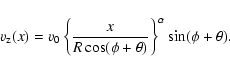
Given a power-law velocity profile of
,
we consider that the gas
moves along straight lines passing through the apex in two opposite
directions.
Given a power-law velocity profile of
 ,
the jet velocity along the line of sight can be written as
,
the jet velocity along the line of sight can be written as
 |
(1) |
![\begin{figure}
\par\includegraphics[width=6.8cm,clip]{0189fig8.eps} \end{figure}](/articles/aa/full/2005/29/aa0189-03/Timg113.gif) |
Figure 8:
Sketch of the biconical jet model.
The z and x axes correspond to the line of sight
and the jet axis projected on the plane of the sky,
respectively.
An observer lies at ,
and the x-y plane corresponds to the
plane of the sky.
|
| Open with DEXTER |
Here we adopt v0 of 14.4 km s-1 from the 3D-velocity of the SW maser
(Table 4)
and its distance of 21 AU from the 1.6 km s-1 spot for R.
We believe that this assumption is reasonable when we consider other results from
VLBA proper motions studies in low- and intermediate-mass YSOs
(IRAS 05413-0104: 64  22 km s-1 at a distance of 40 AU from the expansion center
(Claussen et al. 1998),
S106 FIR: 25-40 km s-1 at 25 AU (Furuya et al. 2000),
IRAS 21391+5802:
42 km s-1 at 20 AU (Patel et al. 2000),
NGC 2071 IRS3: 22-42 km s-1 at 260 AU (Seth et al. 2002)).
We thus have the following four free parameters:
PA of the projected jet axis to the plane of the sky
(i.e., PA of x-axis),
,
22 km s-1 at a distance of 40 AU from the expansion center
(Claussen et al. 1998),
S106 FIR: 25-40 km s-1 at 25 AU (Furuya et al. 2000),
IRAS 21391+5802:
42 km s-1 at 20 AU (Patel et al. 2000),
NGC 2071 IRS3: 22-42 km s-1 at 260 AU (Seth et al. 2002)).
We thus have the following four free parameters:
PA of the projected jet axis to the plane of the sky
(i.e., PA of x-axis),
,
 and .
By definition, we can give constraints of
and .
By definition, we can give constraints of
 and
and
 .
To apply such a model, we selected 3 possible axes of
.
To apply such a model, we selected 3 possible axes of
 and
and
 which we refer to as, respectively,
A1-A2, B1-B2 and C1-C2 (see Fig. 9).
Note that
which we refer to as, respectively,
A1-A2, B1-B2 and C1-C2 (see Fig. 9).
Note that
 is the PA of the line connecting
the reference spot and the SW maser, and
that B1-B2 and C1-C2 are parallel to the two pairs of CO outflow lobes
(see Fig. 3 of BFT95).
As for the power-law indices of the jet velocity,
we considered representative values of
is the PA of the line connecting
the reference spot and the SW maser, and
that B1-B2 and C1-C2 are parallel to the two pairs of CO outflow lobes
(see Fig. 3 of BFT95).
As for the power-law indices of the jet velocity,
we considered representative values of
 and -1which characterize constant velocity, accelerating and decelerating jets,
respectively.
and -1which characterize constant velocity, accelerating and decelerating jets,
respectively.
![\begin{figure}
\par\includegraphics[angle=-90,width=7.1cm,clip]{0189fig9.eps} \end{figure}](/articles/aa/full/2005/29/aa0189-03/Timg120.gif) |
Figure 9:
Guide map showing the 3 jet axes that have been taken as cutting lines
in the position-velocity diagrams (see text; Fig. 10).
To avoid confusion, we present only an outline of each single lobe of the jet.
The position angles of the 3 jet axes in the upper panel are
for the axis with the labels of A1 and A2,
 for B1 and B2, and
for C1 and C2.
for B1 and B2, and
for C1 and C2.
|
| Open with DEXTER |
![\begin{figure}
\par\includegraphics[width=8.1cm,clip]{0189f10.eps} \end{figure}](/articles/aa/full/2005/29/aa0189-03/Timg121.gif) |
Figure 10:
Comparison of the radial velocities from the biconical jet model
with the observed LSR-velocities in the position-velocity (PV) diagram
along the A1-A2 axis.
Here we plotted all of the maser spots detected in the 4 epoch observations.
The vertical and horizontal dashed lines, respectively, represent the positions
of the reference 1.6 km s-1 spot.
Expected blue- and redshifted radial velocity regions from the model
are hatched with blue and red, respectively (see text).
|
| Open with DEXTER |
We compared the observed and calculated velocities
in position-velocity (PV) diagrams:
the black dots in Fig. 10 represent the PV distribution of
the masers along the A1-A2 axis.
Here we took the LSR-velocity of -1.6 km s-1 as the mean velocity.
Figure 10 clearly tells us that
the systemic velocity of
 =6 km s-1
(see the inserted panel in Fig. 2) which was
derived from the 0.01 pc scale molecular cloud (BFT95)
is not valid for the 10 AU scale maser emitting region.
We started searching for the best-fit parameters from .
We found that only an accelerating jet can explain the observed velocity structure
whereas both constant velocity and decelerating jets cannot.
We thus take
=6 km s-1
(see the inserted panel in Fig. 2) which was
derived from the 0.01 pc scale molecular cloud (BFT95)
is not valid for the 10 AU scale maser emitting region.
We started searching for the best-fit parameters from .
We found that only an accelerating jet can explain the observed velocity structure
whereas both constant velocity and decelerating jets cannot.
We thus take
 ,
leaving us with
two free parameters -
and .
We obtained the best-fit parameters of
,
leaving us with
two free parameters -
and .
We obtained the best-fit parameters of
 ,
and
,
and
 .
The blue- and red hatched regions in the 1st and 3rd quadrants of Fig. 10,
respectively, show the expected LSR-velocity ranges for the blue- and redshifted components.
Although the observed maser emission is not excited all over the expected regions,
a large opening angle such as
.
The blue- and red hatched regions in the 1st and 3rd quadrants of Fig. 10,
respectively, show the expected LSR-velocity ranges for the blue- and redshifted components.
Although the observed maser emission is not excited all over the expected regions,
a large opening angle such as
 is required to explain the velocity structure
in the 1st and 3rd quadrants.
This geometry suggests that the line of sight would match the cone surface
(that is,
is required to explain the velocity structure
in the 1st and 3rd quadrants.
This geometry suggests that the line of sight would match the cone surface
(that is,
 ).
However, the remaining maser spots in the 4th quadrant, which are
Features 13 and 14
(see Fig. 3),
are not consistent with the jet model predictions.
).
However, the remaining maser spots in the 4th quadrant, which are
Features 13 and 14
(see Fig. 3),
are not consistent with the jet model predictions.
Since only the accelerating jet explains the velocity structure,
we extended our analysis to the remaining two axes of B1-B2 and C1-C2,
keeping
.
The best-fit parameters for the B1-B2, and C1-C2 cases are
essentially the same as
those obtained from the A1-A2 in the following three senses:
In addition, we performed further analysis by changing the PA through 5increments,
realizing the following points which might jeopardize the above conclusion:
- (a) There is a 4 order of magnitude difference in the spatial
scales between our VLBA images and CO (2-1) maps.
- (b) There is no clear association of CO outflows with known driving source(s)
(Sect. 4.1; BFT95; Chini et al. 2001).
- (c) The maser emission does not trace the whole of the outflowing gas.
Nonetheless,
the analysis with 5
PA steps showed
that the above results from (i) to (iii) are valid, and
that no range of PA other than from
 to
to
 can be
taken.
can be
taken.
Of the available observations of this region, our high resolution data has
the best opportunity to discern individual sources of outflow.
We stress that a single jet model cannot
explain the PV structure of Features 13 and 14 which
are located at the most western portion of the chain of the MAIN maser features,
but show a clear velocity gap with respect to the coherent velocity structure from
Features 3 to 12 (see Fig. 3).
Can they be used to pinpoint additional sources of outflow,
perhaps associated with the other jet-like CO outflows from the region?
We examined the velocity structure of the discordant spots
in terms of a "multiple jet scenario''
by applying the above
"single jet model'' to "residual PV diagrams''.
We subtracted maser spots in the hatched regions in Fig. 10.
In addition, we subtracted all the SW spots, assuming that such spots are
associated with the "main'' jet.
Hence, the "residual spots'' consist of all the spots in Features 13 and 14,
and most of the spots in Features 1-3.
"Residual PV diagrams'' were made along position angles incremented by
 ,
including all the CO outflow position angles.
Given the same driving source as the "main'' jet,
one of the second jet lobes must lie to the NW,
which might be characterized by a
PA
,
including all the CO outflow position angles.
Given the same driving source as the "main'' jet,
one of the second jet lobes must lie to the NW,
which might be characterized by a
PA
 ,
,
 and
and
 ,
but with no symmetrically placed lobe.
We are unable to convincingly associate the residual spots with any particular
flow geometry or additional discrete source.
We speculate that
the residual spots are being excited in some shocked regions associated with the
"main'' jet.
,
but with no symmetrically placed lobe.
We are unable to convincingly associate the residual spots with any particular
flow geometry or additional discrete source.
We speculate that
the residual spots are being excited in some shocked regions associated with the
"main'' jet.
We summarize our jet model analysis
by combining the results from i) to iii) with those from the
"residual PV'' analysis:
- 1.
- The majority of the H2O masers are most likely
to be associated with an accelerating biconical jet
whose projected axis has a PA of
 ,
and
whose opening angle is larger than about
.
,
and
whose opening angle is larger than about
.
- 2.
- The cone surface enclosing the jet almost matches the line of sight.
- 3.
- We could not clearly explain the origin of the remaining maser spots,
and speculate that they are being excited in more complex jet-cloud interactions.
We suggest that MMS1 is probably a single star and is the source of the
flow exciting the masers lying near it.
If there has been no precession(s) of the maser jet and CO outflow(s),
our results indicate that the maser jet is most closely
associated with the NE-SW
pair of the IHV CO lobes because their axes are almost parallel.
The large opening angle of
at a distance of 21 AU
from the assumed expansion center
is similar to that measured in the intermediate-mass YSO of IRAS 21391+5802
by Patel et al. (2000)-these authors reported an opening angle
of
at the 150 AU point from the star.
Interestingly these results are also consistent with those from
high-mass (proto)stars
(Shepherd et al. 2001, and references therein)
rather than low-mass protostars where highly collimated CO outflows
are generally seen (Richer et al. 2000, and references therein).
We suggest that higher luminosity
YSOs tend to have poorly collimated jets,
and that a similar jet morphology holds
for intermediate-mass stars.
The conclusion that the masers accelerate agrees
with observations of other intermediate-mass YSOs
such as S106 FIR (Furuya et al. 1999)
and IRAS 21391+5802 (Patel et al. 2000).
In addition, this conclusion does not disagree with that from the
high-mass star forming region W49N where Gwinn, Moran & Reid (1992)
reported that the expansion velocity of the masering gas has a constant
velocity of 18 km s-1 up to 0.1 pc from the center,
beyond which their velocity increases to more than 200 km s-1.
Given the complexity of the region
seen in the CO maps (BFT95) and the near-IR image (Chen et al. 1997),
we believe that sub-arcsecond resolution imaging of the
CO outflow and continuum emissions with radio interferometers
will associate jets and outflows with their driving sources.
These interferometric observations will fill the spatial resolution gap
between our AU scale VLBI view of the masers and the 0.01 pc scale
single-dish telescope view of the CO outflows.
As we have mentioned,
IRAS 20050+2720 has displayed H2O maser emission at
and -78 km s-1
since 2003 January, which was not seen during our observations (Sect. 4.2.2).
Subsequent monitoring observations using the Green Bank 100-m telescope
(Wootten, private communication) showed that these emissions flared
to 20 Jy in 2004 October.
Together with sub-arcsecond interferometric observations, further VLBA H2O maser
studies will help to assess the nature of this multiple
jet-outflow system, which harbors some of the highest velocity outflowing gas
in any star-forming region known to date.
We have performed 4-epoch monthly VLBA observations of the H2O masers in the intermediate-mass
protostar IRAS 20050+2720 MMS1 together with aperture synthesis observations
of 3 mm continuum emission with the OVRO array.
The main results of this study are summarized as follows.
- 1.
- From the VLBA images taken with all 10 antennae,
we found the two groups of low-velocity H2O maser spots toward the
bright millimeter continuum emission peak.
One group (the MAIN group) showed intense emission around the cloud velocity,
the other (the SW feature) was located at a projected distance of 18.2 AU south-west of the MAIN.
The OVRO 3-mm images clearly showed that the bulk of millimeter
continuum emission (MMS1) is associated with the low-velocity masers.
- 2.
- Using only the south-western antennae of the VLBA,
we have succeeded in detecting EHV maser emission blueshifted
by 99 km s-1 to the cloud velocity.
The EHV emission is located at 4400 mas east and
709 mas south of the low-velocity emission.
Considering the large 3D separation between the MAIN and EHV features,
and the proper motion of the EHV toward the MAIN,
we conclude that the EHV emission is not associated with the low-velocity emission.
A distinct millimeter continuum source appears to be associated with the
EHV masers, which
we speculate is the driving source of the
EHV emission and which could be an extremely young protostar.
- 3.
- The overall structure of the masers in the MAIN group did not
change over the 4 epochs.
On the other hand,
we found that the projected separation between the MAIN group and the
SW feature increased by 1.13 mas over the 4 epochs,
which corresponds to a transverse velocity of 14.4 km s-1.
This increment of the separation indicates proper motion(s)
of spatially localized masing gas in the MAIN group and/or the SW Features.
- 4.
- From the analysis of the velocity field of the masers,
we conclude
that the majority of the H2O masers in IRAS 20050+2720 MMS1 are likely to be
associated with an accelerating biconical jet whose opening angle is
approximately
at a distance of 21 AU from the central star.
The presence of such accelerating jet indicates that
the central protostar is driving the powerful jet.
Moreover, the obtained large opening angle of the jet would support
the hypothesis that poor jet collimation is an inherent property of luminous YSOs.
Acknowledgements
We are grateful to all of the staff at the VLBA, VLA, and OVRO.
R.S.F. thanks C. M. Walmsley for discussion and encouragement.
R.S.F. was supported by the postdoctoral fellowship program at
INAF, Osservatorio Astrofisico di Arcetri, Italy.
Research at the Owens Valley Radio Observatory is supported
by the National Science Foundation through NSF grant AST 02-28955.
- Andr
 , P., Ward-Thompson, D., & Barsony, M. 1993, ApJ,
406, 122 [NASA ADS] [CrossRef] (In the text)
, P., Ward-Thompson, D., & Barsony, M. 1993, ApJ,
406, 122 [NASA ADS] [CrossRef] (In the text) - Andr
, P., Ward-Thompson, D., & Barsony, M. 2000, in
Protostars and Planets IV, ed. V. Mannings, A. P. Boss, & S. S.
Russell (Tucson: University of Arizona Press), 59
(In the text)
-
Bachiller, R. 1996, ARA&A, 34, 111 [NASA ADS] (In the text)
-
Bachiller, R., Fuente, A., & Tafalla, M. 1995, ApJ, 445, L51 [NASA ADS] [CrossRef]
(BFT95)
- Brand, J.,
Cesaroni, R., Caselli, P., et al. 1994, A&AS, 103, 541 [NASA ADS] (In the text)
- Chen, H., Tafalla,
M., Greene, T. P., Myers, P. C., & Wilner, D. J. 1997, ApJ,
475, 163 [NASA ADS] [CrossRef] (In the text)
- Chini, R.,
Ward-Thompson, D., Kirk, J. M., et al. 2001, A&A, 369, 155 [EDP Sciences] [NASA ADS] (In the text)
- Claussen,
M. J., Wilking, B. A., Benson, P. J., et al. 1996, ApJS, 106,
111 [NASA ADS] [CrossRef] (In the text)
- Claussen,
M. J., Marvel, K. B., Wootten, A., & Wilking, B. A. 1998, ApJ,
507, L79 [NASA ADS] [CrossRef] (In the text)
- Condon, J. J.
1997, PASP, 109, 166 [NASA ADS] [CrossRef] (In the text)
- Felli, M.,
Palagi, F., & Tofani, G. 1992, A&A, 255, 293 [NASA ADS] (In the text)
- Fiebig, D.,
Duschl, W. J., Menten, K. M., & Tscharnuter, W. M. 1996,
A&A, 310, 199 [NASA ADS] (In the text)
- Furuya, R. S.,
Kitamura, Y., Saito, M., Kawabe, R., & Wootten, H. A. 1999,
ApJ, 525, 821 [NASA ADS] [CrossRef] (In the text)
- Furuya, R. S.,
Kitamura, Y., Wootten, H. A., et al. 2000, ApJ, 542, L135 [NASA ADS] [CrossRef] (In the text)
- Furuya, R. S.,
Kitamura, Y., Wootten, H. A., Claussen, M. J., & Kawabe, R.
2001, ApJ, 559, L143 [NASA ADS] [CrossRef] (In the text)
- Furuya, R. S.,
Kitamura, Y., Wootten, H. A., Claussen, M. J., & Kawabe, R.
2003, ApJS, 143, 71 [NASA ADS] (In the text)
- Hofner, P.,
& Churchwell, E. 1996, A&AS, 120, 283 [EDP Sciences] [NASA ADS] (In the text)
- Gwinn, C. R.,
Moran, J. M., & Reid, M. J. 1992, ApJ, 393, 149 [NASA ADS] [CrossRef]
- Molinari,
S., Brand, J., Cesaroni, R., & Palla, F. 1996, A&A, 308,
573 [NASA ADS] (In the text)
-
Moscadelli, L., Cesaroni, R., & Rioja, M. J. 2000, A&A,
360, 663 [NASA ADS] (In the text)
- Palla, F., Brand,
J., Comoretto, G., Felli, M., & Cesaroni, R. 1991, A&A,
246, 249 [NASA ADS] (In the text)
- Palumbo, G.
G. C., Scappini, F., Pareschi, G., et al. 1994, MNRAS, 266,
123 [NASA ADS] (In the text)
- Patel, N. A.,
Greenhill, L. J., Herrnstein, J., et al. 2000, ApJ, 538, 268 [NASA ADS] [CrossRef] (In the text)
- Richer, J. S.,
Shepherd, D. S., Cabrit, S., Bachiller, R., & Churchwell, E.
2000, in Protostars and Planets IV, ed. V. Mannings, A. P. Boss,
& S. S. Russell (Tucson: University of Arizona Press), 867
(In the text)
- Seth, A. C.,
Greenhill, L. J., & Holder, B. P. 2002, ApJ, 581, 325 [NASA ADS] [CrossRef] (In the text)
- Shepherd,
D. S., Claussen, M. J., & Kurtz, S. E. 2001, Science, 292,
1513 [NASA ADS] [CrossRef] (In the text)
- Terebey, S.,
Vogel, S. N., & Myers, P. C. 1992, ApJ, 390, 181 [NASA ADS] [CrossRef] (In the text)
-
Torrelles, J. M., G
 mez, J. F., Rodr
 guez, L. F., et al. 1998, ApJ, 505, 756 [NASA ADS] [CrossRef] (In the text)
 - Walker, R. C.,
Matsakis, D. N., & Garcia-Barreto, J. A. 1982, ApJ, 255,
128 [NASA ADS] [CrossRef] (In the text)
- Walker, R. C.
1981, AJ, 86, 1323 [NASA ADS] [CrossRef] (In the text)
- Wilking, B.
A., Blackwell, J. H., Mundy, L. G., & Howe, J. E. 1989, ApJ,
345, 257 [NASA ADS] [CrossRef] (In the text)
- Wilking, B.
A., Claussen, M. J., Benson, P. J., et al. 1994, ApJ, 431,
L119 [NASA ADS] [CrossRef] (In the text)
- Wilner, D. J.,
& Welch, W. J. 1994, ApJ, 427, 898 [NASA ADS] [CrossRef] (In the text)
- Wootten, A.
1989, ApJ, 337, 858 [NASA ADS] [CrossRef] (In the text)
Copyright ESO 2005
![\begin{figure}
\par\includegraphics[angle=-90,width=15cm,clip]{0189fig1.ps} \end{figure}](/articles/aa/full/2005/29/aa0189-03/img42.gif)
![\begin{figure}
\par\includegraphics[angle=-90,width=8.6cm,clip]{0189fig2.eps} \end{figure}](/articles/aa/full/2005/29/aa0189-03/img60.gif)
![\begin{figure}
\par\includegraphics[angle=-90,width=17cm,clip]{0189fig3.eps} \end{figure}](/articles/aa/full/2005/29/aa0189-03/img69.gif)
![\begin{figure}
\par\includegraphics[width=5.8cm,clip]{0189f4a.eps}\hspace*{4mm}
...
...cm}\includegraphics[width=5.8cm,clip]{0189f4g.eps}\hspace*{3.5cm}}
\end{figure}](/articles/aa/full/2005/29/aa0189-03/img85.gif)
![\begin{figure}
\par\includegraphics[width=13cm,clip]{0189fig5.eps} \end{figure}](/articles/aa/full/2005/29/aa0189-03/img86.gif)
![\begin{figure}
\par\mbox{\hspace*{8mm}\includegraphics[width=4cm,clip]{0189f6a.e...
...ip]{0189f6f.eps} \includegraphics[width=5.6cm,clip]{0189f6g.eps} }
\end{figure}](/articles/aa/full/2005/29/aa0189-03/img96.gif)
![\begin{figure}
\par\mbox{\includegraphics[angle=-90,width=10.1cm,clip]{0189f7a.eps} \includegraphics[angle=-90,width=4.3cm,clip]{0189f7b.eps} }
\end{figure}](/articles/aa/full/2005/29/aa0189-03/img97.gif)
![\begin{figure}
\par\includegraphics[width=6.8cm,clip]{0189fig8.eps} \end{figure}](/articles/aa/full/2005/29/aa0189-03/img113.gif)
![\begin{figure}
\par\includegraphics[angle=-90,width=7.1cm,clip]{0189fig9.eps} \end{figure}](/articles/aa/full/2005/29/aa0189-03/img120.gif)
![\begin{figure}
\par\includegraphics[width=8.1cm,clip]{0189f10.eps} \end{figure}](/articles/aa/full/2005/29/aa0189-03/img121.gif)
 for B1-B2 and
 for C1-C2),
in other words, the PA would have an uncertainty of
for C1-C2),
in other words, the PA would have an uncertainty of
 .
.
 for B1-B2, and
 for C1-C2),
namely, the SW masers lie at the either of the two edges of the cone.
for C1-C2),
namely, the SW masers lie at the either of the two edges of the cone.