Contents

• The projection factor of ${\delta }$ Cephei
• 1 Introduction
• 2 Application of the BW method to ${\delta }$ Cep
• 3 Discussion
• References
• 4 Online Material

A&A 438, L9-L12 (2005)
DOI: 10.1051/0004-6361:200500139

The projection factor of ${\delta }$ Cephei

A calibration of the Baade-Wesselink method using the CHARA Array

A. Mérand¹ - P. Kervella¹ - V. Coudé du Foresto¹ - S. T. Ridgway^1,2,3 - J. P. Aufdenberg² - T. A. ten Brummelaar³ - D. H. Berger³ - J. Sturmann³ - L. Sturmann³ - N. H. Turner³ - H. A. McAlister³

1 - LESIA, UMR8109, Observatoire de Paris-Meudon, 5, place Jules Janssen, 92195 Meudon Cedex, France
2 - National Optical Astronomical Observatory 950 North Cherry Avenue, Tucson, AZ 85719, USA
3 - Center for High Angular Resolution Astronomy, Georgia State University, PO Box 3965, Atlanta, Georgia 30302-3965, USA

Received 6 May 2005 / Accepted 7 June 2005

Abstract
Cepheids play a key role in astronomy as standard candles for measuring intergalactic distances. Their distance is usually inferred from the period-luminosity relationship, calibrated using the semi-empirical Baade-Wesselink method. Using this method, the distance is known to a multiplicative factor, called the projection factor. Presently, this factor is computed using numerical models - it has hitherto never been measured directly. Based on our new interferometric measurements obtained with the CHARA Array and the already published parallax, we present a geometrical measurement of the projection factor of a Cepheid, ${\delta }$ Cep. The value we determined, p=1.27 $\pm$ 0.06, confirms the generally adopted value of p=1.36 within 1.5 sigmas. Our value is in line with recent theoretical predictions of Nardetto et al. (2004, A&A, 428, 131).

Key words: techniques: interferometric - stars: variables: Cepheids - stars: individual: ${\delta }$ Cep - cosmology: distance scale

1 Introduction

Cepheid stars are commonly used as cosmological distance indicators, thanks to their well-established period-luminosity law (P-L). This remarkable property has turned these supergiant stars into primary standard candles for extragalactic distance estimations. With intrinsic brightnesses of up to 100 000 times that of the Sun, Cepheids are easily distinguished in distant galaxies (up to about 30 Mpc distant). As such, they are used to calibrate the secondary distance indicators (supernovae, etc...) that are used to estimate even larger cosmological distances. For instance, the Hubble Key Project to measure the Hubble constant H₀ (Freedman et al. 2001) is based on the assumption of a distance to the LMC that was established primarily using Cepheids. Located at the very base of the cosmological distance ladder, a bias on the calibration of the Cepheid P-L relation would impact our whole perception of the scale of the Universe.

1.1 Period-luminosity calibration

The P-L relation takes the form $\log L = \alpha \log P + \beta$, where L is the (absolute) luminosity, P the period, $\alpha$ the slope, and $\beta$ the zero point. The determination of $\alpha$ is straightforward: one can consider a large number of Cepheids in the LMC, located at a common distance from us. Calibrating the zero-point $\beta$ is a much more challenging task, as it requires an independent distance measurement to a number of Cepheids. Ideally, one should measure directly their geometrical parallaxes, in order to obtain their absolute luminosity. Knowing their variation period, $\beta$would then come out easily. However, Cepheids are rare stars: only a few of them are located in the solar neighborhood, and these nearby stars are generally too far away for precise parallax measurements, with the exception of ${\delta }$ Cep.

1.2 The Baade-Wesselink method

The most commonly used alternative to measure the distance to a pulsating star is the Baade-Wesselink (BW) method. Developed in the first part of the 20th century (Wesselink 1946; Baade 1926), it utilizes the pulsational velocity  $V_{{\rm puls.}}$ of the surface of the star and its angular size. Integrating the pulsational velocity curve provides an estimation of the linear radius variation over the pulsation. Comparing the linear and angular amplitudes of the Cepheid pulsation gives directly its distance. The most recent implementation (Kervella et al. 2004) of the BW method makes use of long-baseline interferometry to measure directly the angular size of the star.

Unfortunately, spectroscopy measures the apparent radial velocity  $V_{{\rm rad.}}$, i.e. the Doppler shift of absorption lines in the stellar atmosphere, projected along the line of sight and integrated over the stellar disk. This is where p, a projection factor, has to be introduced, which is defined as $p=V_{{\rm puls.}}/V_{{\rm rad.}}$. The general BW method can be summarized in the relation:

$$% \theta(T)-\theta(0) = - 2~\frac{p}{d}\int_0^T \left(V_{{\rm rad.}}(t)-V_\gamma \right)~{\rm d}t$$ (1)

where d is the distance, p the projection factor, $\theta$ the angular diameter and $V_\gamma$ the systematic radial velocity. There are in fact many contributors to the p-factor. The main ones are the sphericity of the star (purely geometrical) and its limb darkening (due to the stellar atmosphere structure). A careful theoretical calculation of p requires modeling dynamically the formation of the absorption line in the pulsating atmosphere of the Cepheid (Parsons 1972; Sabbey et al. 1995; Nardetto et al. 2004).

Until now, distance measurements to Cepheids used a p-factor value estimated from numerical models. Looking closely at Eq. (1), it is clear that any uncertainty on the value of p will create the same relative uncertainty on the distance estimation, and subsequently to the P-L relation calibration. In other words, the Cepheid distance scale relies implicitly on numerical models of these stars. But how good are the models? To answer this question, one should confront their predictions to measurable quantities. Until now, this comparison was impossible due to the difficulty to constrain the two variables $\theta(T)$ and d from observations, i.e. the angular diameter and the distance.

Among classical Cepheids, ${\delta }$ Cep (HR 8571, HD 213306) is remarkable: it is not only the prototype of its kind, but also the Cepheid with the most precise trigonometric parallax currently available, obtained recently using the FGS instrument aboard the Hubble Space Telescope (Benedict et al. 2002). This direct measurement of the distance opens the way to the direct measurement (with the smallest sensitivity to stellar models) of the p factor of ${\delta }$ Cep, provided that high-precision angular diameters can be measured by interferometry.

2 Application of the BW method to ${\delta }$ Cep

To achieve this goal, interferometric observations were undertaken at the CHARA Array (ten Brummelaar et al. 2003,2005), in the infrared K' band ( $1.95~\mu {\rm m}\leq \lambda \leq 2.3~\mu {\rm m}$) with the Fiber Linked Unit for Optical Recombination (Coudé du Foresto et al. 2003) (FLUOR) using two East-West baselines of the CHARA Array: E1-W1 and E2-W1, with baselines of 313 and 251 m respectively. Observations took place during summer 2004 for E2-W1 (seven nights between JD  $2\ 453\ 216$ and JD  $2\ 453\ 233$) and Fall 2004 for E1-W1 (six consecutive nights, from JD  $2\ 453\ 280$ to JD  $2\ 453\ 285$). The pulsation phase was computed using the following period and reference epoch (Moffett & Barnes 1985): P=5.366316 d, $T_0= 2\ 453\ 674.144$ (Julian date), the 0-phase being defined at maximum light in the V band. The resulting phase coverage is very good for the longest baseline (E1-W1), while data lack at minimum diameter for the smaller one (E2-W1)

The FLUOR Data reduction software (DRS) (Coudé du Foresto et al. 1997), was used to extract the squared modulus of the coherence factor between the two independent apertures. All calibrator stars were chosen in a catalogue computed for this specific purpose (Mérand et al. 2005) (see Table 1). Calibrators chosen for this work are all K giants, whereas ${\delta }$ Cep is a G0 supergiant. The spectral type difference is properly taken into account in the reduction, even though it has no significant influence on the final result. The interferometric transfer function of the instrument was estimated by observing calibrators before and after each ${\delta }$ Cep data point. The efficiency of CHARA/FLUOR was consistent between all calibrators and stable over the night around 85%. Data that share a calibrator are affected by a common systematic error due to the uncertainty of the a priori angular diameter of this calibrator. In order to interpret our data properly, we used a specific formalism (Perrin 2003) tailored to propagate these correlations into the model fitting process. Diameters are derived from the visibility data points using a full model of the FLUOR instrument including the spectral bandwidth effects (Kervella et al. 2003). The stellar center-to-limb darkening is corrected using a model intensity profile taken from tabulated values (Claret 2000) with parameters corresponding to ${\delta }$ Cep ( $T_{{\rm eff}}=6000~{\rm K}$, $\log g=2.0$ and solar metallicity). The limb darkened (LD) angular diameter comes out 3% larger than its uniform disk (UD) counterpart.

 

 

Table 1: Calibrators with spectral type, uniform disk angular diameter in K band (in milliarcsecond) and baseline (Mérand et al. 2005).

	S. type	UD diam. (mas)	Baseline
HD 2952	K0III	$0.938\pm 0.013$	W1-E1
HD 138852	K0III-IV	$0.952\pm 0.012$	W1-E1
HD 139778	K1III:	$1.072\pm 0.014$	W1-E2
HD 186815	K2III	$0.713\pm 0.009$	W1-E2
HD 206349	K1II-III	$0.869\pm 0.011$	W1-E1, W1-E2
HD 206842	K1III	$1.214\pm 0.016$	W1-E2
HD 214995	K0III:	$0.947\pm 0.013$	W1-E1
HD 216646	K0III	$1.051\pm 0.015$	W1-E1, W1-E2
HD 217673	K1.5II	$1.411\pm 0.020$	W1-E2

The theoretical correction for LD has only a weak influence on the p-factor determination, since that determination is related to a diameter variation. For example, based on our data set, a general bias of 5% in the diameters (due to a wrongly estimated limb darkening) leads to a bias smaller than 1% in terms of the p-factor. Differential variations of the LD correction during the pulsation may also influence the projection factor: comparison between hydrodynamic and hydrostatic simulations (Marengo et al. 2003) showed negligible variations. An accuracy of 0.2% on the angular diameters for a given baseline is required to be sensitive to dynamical LD effects. This is close to, but still beyond, the best accuracy that we obtained on the angular diameter with a single visibility measurement: 0.35% (median 0.45%).

Among the various sets of measurements of the radial velocity  $V_{{\rm rad.}}(t)$ available for ${\delta }$ Cep, we chose measurements from Bersier et al. (1994) and Barnes et al. (2005). These works offer the best phase coverage, especially near the extrema, in order to accurately estimate the associated photospheric amplitude. In order not to introduce any bias due to a possible mismatch in the radial velocity zero-point between the two data sets, we decided to reduce them separately and then combine the resulting p-factor. An integration over time is required to obtain the photospheric displacement (see Eq. (1)). This process is noisy for unequally spaced data points: the radial velocity profile was smoothly interpolated using a periodic cubic spline function.

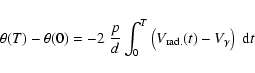
Fitting the inferred photospheric displacement and observed angular diameter variations, we adjust three parameters: the mean angular diameter  $\overline{\theta}$, a free phase shift $\phi_0$ and the projection factor p (see Fig. 1). The mean angular diameter is found to be 1.475 $\pm$ 0.004 mas (milliarcsecond) for both radial velocity data sets. Assuming a distance of 274 $\pm$ 11 pc (Benedict et al. 2002), this leads to a linear radius of 43.3 $\pm$ 1.7 solar radii. The fitted phase shift is very small in both cases (of the order of 0.01). We used the same parameters (Moffett & Barnes 1985) to compute the phase from both observation sets and considering that they were obtained more than ten years apart, this phase shift corresponds to an uncertainty in the period of approximately five seconds. We thus consider the phase shift to be reasonably the result of uncertainty in the ephemeris.

Figure 1: Radial velocity smoothed using splines. A. Radial velocity data points, as a function of pulsation phase (0-phase defined as the maximum of light). This set was extracted using a cross-correlation technique (Bersier et al. 1994). The solid line is a 4-knot periodic cubic spline fit. B. Residuals of the fit.

Figure 2: p-factor determination. A. Our angular diameter measurements (points). Crosses correspond to the medium baseline (E2-W1), while circles correspond to the largest baseline (E1-W1). The continuous line is the integration of the 4-knots periodic cubic spline fitted to the radial velocities (Fig. 1). Integration parameters: $\overline{\theta}=1.475~{\rm mas}$, p=1.269 and $d=274~{\rm pc}$. B. Residuals of the fit.

The two different radial velocity data sets lead to a consolidated value of p=1.27 $\pm$ 0.06, once again assuming a distance of 274 $\pm$ $11~{\rm pc}$. The final reduced $\chi^2$ is 1.5. The error bars account for three independent contributions: uncertainties in the radial velocities, the angular diameters and the distance. The first was estimated using a bootstrap approach, while the others were estimated analytically (taking into account calibration correlation for interferometric errors): for p, the detailed error is p=1.273 $\pm$ $0.007_{V{\rm rad.}}$ $\pm$ $0.020_{{\rm interf.}}$ $\pm$ $0.050_{{\rm dist.}}$. The error is dominated by the distance contribution (see Table 2).

 

 

Table 2: Best fit results for p, with the two different radial velocity sets. The third line is a weighted average of the two individual measurements. Fourth and fith lines are the detailed quadratic contribution to the final error bar. Last line gives the final adopted value with the overall error bar. References are: (1) Bersier et al. (1994); and (2) Barnes et al. (2005).

$p\pm\sigma_{\rm Vrad.}$	1.269 $\pm$ 0.008	ref. (1)
	1.280 $\pm$ 0.012	ref. (2)
$p\pm\sigma_{\rm Vrad.}$	1.273 $\pm$ 0.007	consolidated
$\sigma_{\rm interf.}$	$\pm$0.020
$\sigma_{\rm dist.}$	$\pm$0.050
p	1.27 $\pm$ 0.06

3 Discussion

Until now, the p-factor has been determined using models: hydrostatic models (Burki et al. 1982) produced the generally adopted value, p=1.36. First attempts were made by Sabbey et al. (1995) to take into account dynamical effects due to the pulsation. They concluded that the average value of p should be 5% larger than in previous works (1.43 instead of 1.36) and that p is not constant during the pulsation. Because they increased p by 5%, they claimed that distances and diameters have to be larger in the same proportion. More recently Nardetto et al. (2004) computed pspecifically for ${\delta }$ Cep using dynamical models. Different values of p were found, whether one measures diameters in the continuum or in the layer where the specific line is formed. In our case, broad band stellar interferometry (angular diameters are measured in the continuum) these authors suggest p=1.27 $\pm$ 0.01. Concerning the variation of p during the pulsation, they estimate that the error in terms of distance is of the order of 0.2%, smaller than what we would have been able to measure with our interferometric data set. While our estimate, p=1.27 $\pm$ 0.06, is statistically compatible with this recent work, marginally with the widely used p=1.36, and not consistent with the former value p=1.43 at a 2$\sigma$ level. We note that Gieren et al. (2005) have recently derived an expression of the p-factor as a function of the period that predicts a value of 1.47 $\pm$ 0.06 for ${\delta }$ Cep. While this value is in agreement with the modeling by Sabbey et al. (1995), is is slightly larger than the present measurement (by 2.4$\sigma$). As a remark, Gieren et al. obtain a distance of 280 $\pm$ 4 pc for ${\delta }$ Cep, that is slightly larger than Benedict et al.'s (2002) value 274 $\pm$ 11 pc assumed in the present work. Assuming this new distance estimation with our data would result in a p-factor of 1.30 $\pm$ 0.06, bringing the agreement to 2$\sigma$ only.

Our geometrical determination of the p-factor, p=1.27 $\pm$ 0.06, using the IBW method is currently limited by the error bar on the parallax (Benedict et al. 2002). Conversely, assuming a perfectly known p-factor, the uncertainty of the stellar distance determined using the same method would have been only 1.5%, two-times better than the best geometrical parallax currently available. The value we determined for p is statistically compatible with the value generally adopted to calibrate the Cepheid P-L relation in most recent works. It is expected that the distance to approximatively 30 Cepheids will be determined interferometrically in the near future using particularly the CHARA Array and the VLT Interferometer (Glindemann 2005). In order not to limit the final accuracy on the derived distances, theoretical p-factor studies using realistic hydrodynamical codes is necessary. With a better understanding of the detailed dynamics of the Cepheid atmospheres, we will be in a position to exclude a p-factor bias on the calibration of the P-L relation, at a few percent level.

Acknowledgements

We thank P. J. Goldfinger for her assistance during the observations. The CHARA Array was constructed with funding from Georgia State University, the National Science Foundation, the W. M. Keck Foundation, and the David and Lucile Packard Foundation. The CHARA Array is operated by Georgia State University with support from the College of Arts and Sciences, from the Research Program Enhancement Fund administered by the Vice President for Research, and from the National Science Foundation under NSF Grant AST 0307562.

References

 
• Baade, W. 1926, Astron. Nachr., 228, 359
   
• Barnes, J. R., Cameron, A. C., Donati, J.-F., et al. 2005, MNRAS, 357, L1
   
• Benedict, G. F., McArthur, B. E., Fredrick, L. W., et al. 2002, AJ, 124, 1695
   
• Bersier, D., Burki, G., Mayor, M., & Duquennoy, A. 1994, A&A, 108, 25
   
• Burki, G., Mayor, M., & Benz, W. 1982, A&A, 109, 258
   
• Claret, A. 2000, A&A, 363, 1081
   
• Coudé du Foresto, V., Bordé, P. J., Mérand, A., et al. 2003, in Interferometry for Optical Astronomy II, ed. W. A. Traub, Proc. SPIE, 4838, 280
   
• Coudé du Foresto, V., Ridgway, S., & Mariotti, J.-M. 1997, A&A, 121, 379
   
• Freedman, W. L., Madore, B. F., Gibson, B. K., et al. 2001, ApJ, 553, 47
   
• Glindemann, A. 2005, in New Frontiers in Stellar Interferometry, ed. W. A. Traub, Proc. SPIE, 5491, 417
   
• Kervella, P., Nardetto, N., Bersier, D., Mourard, D., & Coudé du Foresto, V. 2004, A&A, 416, 941
   
• Kervella, P., Thévenin, F., Ségransan, D., et al. 2003, A&A, 404, 1087
   
• Marengo, M., Karovska, M., Sasselov, D. D., et al. 2003, ApJ, 589, 968
   
• Mérand, A., Bordé, P., & Coudé du Foresto, V. 2005, 433, 433
   
• Moffett, T. J., & Barnes, T. G. 1985, ApJS, 58, 843
   
• Nardetto, N., Fokin, A., Mourard, D., et al. 2004, A&A, 428, 131
   
• Parsons, S. B. 1972, ApJ, 174, 57
   
• Perrin, G. 2003, A&A, 596, 702
   
• Sabbey, C. N., Sasselov, D. D., Fieldus, M. S., et al. 1995, ApJ, 446, 250
   
• ten Brummelaar, T. A., McAlister, H. A., Ridgway, S. T., et al. 2005, ApJ, accepted
   
• ten Brummelaar, T. A., McAlister, H. A., Ridgway, S. T., et al. 2003, in Interferometry for Optical Astronomy II, ed. W. A. Traub, Proc. SPIE, 4838, 69
   
• Wesselink, A. 1946, Bull. Astron. Inst. Netherlands, 10, 91
  

 

  
4 Online Material

 

 

Table 3: Individal measurements. Columns are (1) date of observation, JD₀ = $2\; 453\; 200.5$; (2) phase; (3, 4) u-v coordinate in meter; (5) squared visibility and error; (6) corresponding limb darkened disk diameter in mas; (7, 10) HD number of calibrators, prior and after the given data point respectivaly, 0 means that there was no calibrator; (8, 9, 11, 12) quantities for computing the correlation matrix (Perrin 2003): $\sigma _{V^2}$ are errors on the estimated visibility of the calibrators.

JD-JD0	$\phi$	U(m)	V(m)	V2 (%)	$\theta_{\rm LD}$ (mas)	${\rm HD}_a$	$\alpha$	$\sigma_{V^2_a}$	${\rm HD}_b$	$\beta$	$\sigma_{V^2_b}$
16.3844	0.289	-246.23	-13.93	$12.09\pm0.58$	$1.539\pm0.014$	206842	0.232	0.0106	217673	0.313	0.0096
16.4051	0.293	-245.91	-41.24	$11.94\pm0.69$	$1.526\pm0.016$	217673	0.354	0.0096	217673	0.322	0.0095
17.3801	0.475	-246.08	-11.83	$12.79\pm0.47$	$1.524\pm0.011$	217673	0.096	0.0102	216646	0.270	0.0114
17.4005	0.478	-246.11	-38.71	$11.89\pm0.37$	$1.529\pm0.009$	216646	0.154	0.0114	216646	0.152	0.0114
18.3443	0.654	-237.44	31.26	$16.33\pm0.48$	$1.489\pm0.010$	216646	0.188	0.0111	216646	0.189	0.0112
18.3630	0.658	-243.62	7.08	$14.64\pm0.43$	$1.499\pm0.009$	216646	0.173	0.0112	216646	0.183	0.0114
18.3935	0.663	-246.44	-33.07	$13.63\pm0.59$	$1.491\pm0.013$	217673	0.373	0.0096	216646	0.177	0.0114
19.3289	0.838	-231.37	47.22	$21.53\pm0.63$	$1.407\pm0.011$	0	-	-	216646	0.474	0.0110
19.3536	0.842	-241.79	15.84	$20.50\pm0.61$	$1.390\pm0.011$	216646	0.209	0.0110	216646	0.262	0.0112
19.3889	0.849	-246.53	-30.66	$17.95\pm0.77$	$1.403\pm0.015$	217673	0.417	0.0098	216646	0.250	0.0114
19.4093	0.853	-243.71	-57.56	$17.59\pm0.86$	$1.399\pm0.016$	216646	0.214	0.0114	217673	0.526	0.0095
21.3301	0.211	-234.72	38.94	$17.02\pm0.57$	$1.484\pm0.012$	216646	0.296	0.0095	0	-	-
28.4176	0.531	-230.78	-99.51	$11.94\pm0.36$	$1.514\pm0.008$	206349	0.111	0.0089	216646	0.153	0.0114
28.4406	0.536	-215.78	-127.18	$12.38\pm0.41$	$1.509\pm0.010$	216646	0.272	0.0114	206349	0.030	0.0083
28.4630	0.540	-196.83	-152.03	$12.49\pm0.47$	$1.517\pm0.011$	216646	0.171	0.0114	206349	0.099	0.0083
28.4848	0.544	-174.70	-173.74	$12.24\pm0.48$	$1.537\pm0.011$	216646	0.060	0.0114	206349	0.169	0.0083
29.3593	0.707	-246.59	-27.63	$15.93\pm0.57$	$1.445\pm0.012$	206842	0.318	0.0106	216646	0.186	0.0114
29.3863	0.712	-242.60	-63.16	$14.92\pm0.49$	$1.451\pm0.010$	216646	0.161	0.0114	216646	0.224	0.0114
29.4074	0.716	-234.58	-90.27	$14.80\pm0.48$	$1.450\pm0.010$	216646	0.385	0.0114	0	-	-
31.3590	0.080	-246.38	-34.41	$15.37\pm0.38$	$1.453\pm0.008$	186815	0.099	0.0071	206349	0.165	0.0090
31.3828	0.084	-242.03	-65.75	$15.39\pm0.40$	$1.441\pm0.008$	206349	0.126	0.0090	216646	0.226	0.0114
31.4433	0.095	-207.08	-139.54	$15.96\pm0.51$	$1.435\pm0.010$	216646	0.415	0.0114	0	-	-
32.3850	0.271	-240.48	-72.01	$12.49\pm0.38$	$1.503\pm0.009$	138852	0.050	0.0094	216646	0.260	0.0114
32.4220	0.278	-221.30	-118.17	$12.68\pm0.44$	$1.500\pm0.010$	216646	0.139	0.0114	216646	0.183	0.0114
32.4470	0.282	-201.55	-146.52	$13.09\pm0.42$	$1.501\pm0.009$	216646	0.168	0.0114	216646	0.152	0.0112
32.4710	0.287	-177.75	-171.09	$12.86\pm0.42$	$1.520\pm0.010$	216646	0.173	0.0112	216646	0.125	0.0110
32.5025	0.293	-140.59	-198.07	$13.78\pm0.43$	$1.523\pm0.010$	216646	0.121	0.0110	216646	0.171	0.0107
33.3435	0.449	-246.55	-21.14	$12.40\pm0.41$	$1.527\pm0.010$	139778	0.062	0.0102	216646	0.245	0.0114
33.3723	0.455	-243.42	-59.13	$11.72\pm0.47$	$1.525\pm0.011$	216646	0.183	0.0114	206349	0.084	0.0089
33.4189	0.463	-221.54	-117.75	$12.58\pm0.45$	$1.502\pm0.010$	216646	0.151	0.0114	216646	0.169	0.0114
33.4404	0.467	-204.89	-142.38	$12.56\pm0.41$	$1.511\pm0.009$	216646	0.315	0.0114	0	-	-
80.3020	0.200	253.48	183.15	$2.41\pm0.12$	$1.491\pm0.005$	185395	0.008	0.0139	216646	0.086	0.0112
80.3295	0.205	220.84	218.17	$2.46\pm0.12$	$1.500\pm0.006$	216646	0.078	0.0112	2952	0.022	0.0112
80.3667	0.212	166.28	257.01	$2.85\pm0.13$	$1.502\pm0.006$	2952	0.046	0.0112	2952	0.049	0.0112
80.3888	0.216	129.38	274.56	$3.20\pm0.13$	$1.498\pm0.006$	2952	0.050	0.0112	2952	0.056	0.0112
80.4145	0.221	83.29	289.27	$3.19\pm0.15$	$1.511\pm0.006$	2952	0.088	0.0112	37128	0.009	0.0409
81.3127	0.388	238.39	200.90	$2.12\pm0.11$	$1.511\pm0.006$	216646	0.040	0.0110	216646	0.051	0.0112
81.3371	0.393	206.72	230.09	$2.28\pm0.12$	$1.514\pm0.006$	216646	0.083	0.0112	2952	0.009	0.0112
81.3739	0.400	149.99	265.47	$2.61\pm0.13$	$1.519\pm0.006$	216646	0.052	0.0112	2952	0.044	0.0112
82.3031	0.573	246.42	191.85	$2.32\pm0.13$	$1.498\pm0.006$	216646	0.053	0.0110	216646	0.049	0.0112
82.3246	0.577	220.02	218.91	$2.45\pm0.12$	$1.501\pm0.006$	216646	0.057	0.0112	2952	0.037	0.0112
82.3611	0.584	166.58	256.84	$2.78\pm0.11$	$1.504\pm0.005$	2952	0.033	0.0112	2952	0.060	0.0112
83.3260	0.764	214.60	223.63	$3.73\pm0.17$	$1.445\pm0.006$	214995	0.026	0.0097	2952	0.107	0.0112
83.3625	0.770	159.85	260.49	$4.29\pm0.18$	$1.444\pm0.006$	2952	0.063	0.0112	2952	0.080	0.0112
83.3878	0.775	116.78	279.31	$4.75\pm0.20$	$1.440\pm0.007$	2952	0.080	0.0112	2952	0.076	0.0112
84.2374	0.933	294.80	103.39	$6.53\pm0.36$	$1.342\pm0.010$	216646	0.171	0.0109	216646	0.139	0.0109
84.2635	0.938	278.68	143.65	$5.77\pm0.32$	$1.359\pm0.009$	216646	0.136	0.0109	216646	0.138	0.0110
84.2855	0.942	259.31	175.36	$5.64\pm0.28$	$1.365\pm0.008$	216646	0.178	0.0110	2952	0.061	0.0112
84.3201	0.949	218.81	219.98	$5.68\pm0.24$	$1.376\pm0.007$	2952	0.101	0.0112	2952	0.088	0.0112
84.3468	0.954	180.34	248.69	$6.29\pm0.27$	$1.371\pm0.008$	2952	0.118	0.0112	2952	0.093	0.0112
85.3490	0.140	172.71	253.33	$3.36\pm0.16$	$1.476\pm0.006$	176598	0.013	0.0105	2952	0.097	0.0112
85.3962	0.149	91.77	287.10	$3.70\pm0.17$	$1.487\pm0.006$	2952	0.066	0.0112	2952	0.053	0.0112