Relativistic Keplerian orbital frequency (
A&A 437, 775-788 (2005)
DOI: 10.1051/0004-6361:20052825
G. Török - Z. Stuchlík
Institute of Physics, Faculty of Philosophy and Science, Silesian University in Opava, Bezrucovo nám. 13, 746 01 Opava, Czech Republic
Received 6 February 2005 / Accepted 8 March 2005
Abstract
Relativistic Keplerian orbital frequency (
![]() )
and related epicyclic frequencies (radial
)
and related epicyclic frequencies (radial
![]() ,
vertical
,
vertical
![]() )
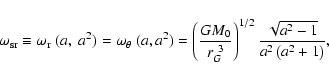
play an important role in the physics of accretion discs orbiting Kerr black holes - quasiperiodic oscillations observed in microquasars can be explained by associated resonant or trapping effects. Because of growing theoretical evidence of the possible existence of naked singularities, we discuss the behaviour of the fundamenal orbital frequencies for Keplerian motion in the field of Kerr naked singularities, primarily in order to find phenomena that could observationally distinguish a hypothetical naked singularity from black holes. Some astrophysically important consequences are sketched, namely the existence of strong resonant frequency for all Kerr naked singularities, with radial and vertical epicyclic frequencies equal and given by the relation
)
play an important role in the physics of accretion discs orbiting Kerr black holes - quasiperiodic oscillations observed in microquasars can be explained by associated resonant or trapping effects. Because of growing theoretical evidence of the possible existence of naked singularities, we discuss the behaviour of the fundamenal orbital frequencies for Keplerian motion in the field of Kerr naked singularities, primarily in order to find phenomena that could observationally distinguish a hypothetical naked singularity from black holes. Some astrophysically important consequences are sketched, namely the existence of strong resonant frequency for all Kerr naked singularities, with radial and vertical epicyclic frequencies equal and given by the relation
![]() =
=
![]() .
.
Key words: black holes physics - X-rays: general
Quasiperiodic oscillations (QPOs) of X-ray brightness have been observed at low-(Hz) and high-(kHz) frequencies in some low-mass X-ray binaries containing neutron stars or black holes; for a review articles see, e.g., McClintock & Remillard (2003) in the case of black hole binaries and van der Klis (2000) in the case of neutron star binaries. Since the peaks of high frequencies are close to the orbital frequency of the marginally stable circular geodesic representing the inner edge of Keplerian discs orbiting black holes (or neutron stars), strong gravity effects must be relevant if trying to explain high frequency QPOs (Abramowicz et al. 2004). In the context of discs oscillations (Nowak & Wagoner 1991; Okazaki et al. 1987; Nowak & Wagoner 1992) both the warped discs (trapped) oscillations (Kato 2004a; Kato & Fukue 1980) and resonant oscillations (Abramowicz et al. 2004; Abramowicz & Kluzniak 2001) has been considered for explaining QPOs.
Usually, in the kHz QPOs the power spectrum shows twin peaks with frequencies correlated to their X-ray intensity and the peak separation almost constant (see, e.g., Zhang et al. 1988; van der Klis et al. 1997; Strohmayer et al. 1996; Ford et al. 1997).
In the case of microquasars containing stellar mass black holes, the observed ratio of the twin peak frequencies is exactly, or almost exactly, 3:2; therefore, some resonant effects are probably involved in oscillating accretion discs of microquasars (Kluzniak & Abramowicz 2001,2000)![]() . It was shown that the parametric resonance of vertical and radial oscillations at epicyclic frequencies related to the Keplerian motion could be the most probable explanation of the observed microquasars phenomena (Török et al. 2005). On the other hand, the forced resonance of the epicyclic frequencies or some other kind of resonance with ratios given by small integral numbers, e.g., 2:1, 3:1, 5:2, etc. could also explain observed QPOs frequencies (with the same 3:2 ratio), if combinational ("beat'') frequencies are considered (Török et al. 2005; Aschenbach 2004; Abramowicz & Kluzniak 2001). The puzzle of this 3:2 ratio kHz frequencies has still not been definitely solved and other possible explanations, like warped-disc oscillations (see Kato 2004b) or simple p-mode oscillations (Rezzolla 2004), can not be exluded.
. It was shown that the parametric resonance of vertical and radial oscillations at epicyclic frequencies related to the Keplerian motion could be the most probable explanation of the observed microquasars phenomena (Török et al. 2005). On the other hand, the forced resonance of the epicyclic frequencies or some other kind of resonance with ratios given by small integral numbers, e.g., 2:1, 3:1, 5:2, etc. could also explain observed QPOs frequencies (with the same 3:2 ratio), if combinational ("beat'') frequencies are considered (Török et al. 2005; Aschenbach 2004; Abramowicz & Kluzniak 2001). The puzzle of this 3:2 ratio kHz frequencies has still not been definitely solved and other possible explanations, like warped-disc oscillations (see Kato 2004b) or simple p-mode oscillations (Rezzolla 2004), can not be exluded.
At any rate, strong observational evidence supports the astrophysical relevance of the disc oscillation concept introduced during the eighties (for a review of the concept itself see, e.g., Kato et al. 1998). The mechanisms for triggering the oscillations in epicyclic frequencies were treated successfully both for thin (see Kato et al. 1998) and thick discs (e.g., Matsumoto et al. 1989; Rezzolla 2004; Abramowicz et al. 2003). Nevertheless, sophisticated three-dimensional magnetohydrodynamic simulations (3-MHD) of accretion flows usually do not show any twin peak kHz QPOs resembling those observed (De Villiers et al. 2003; Igumenshchev et al. 2003, and others). Only very recently Kato (2004c) has reported a view of the 3:2 twin peaks in 3-MHD simulations. In addition, it has recently been shown by Bursa et al. (2004) that the possible resonant oscillations of the torus could be directly observable in X-ray modulation when they occur in the inner parts of accretion flow around a black hole or neutron star, even if the source of radiation is steady and perfectly axisymmetric.
Apparently, the vertical and radial epicyclic frequencies of the Keplerian motion play a crucial role for both thin Keplerian discs and thick toroidal discs. Their properties have been extensively studied in the case of accretion discs orbiting Kerr black holes both in works mentioned above and in many others, yet continue to be very hot outstanding topic in recent astrophysics. On the other hand, it is natural to extend the concept of disc oscillations in the epicyclic frequencies around other physical objects.
According to the cosmic censorship hypothesis (Penrose 1969) and the uniqueness black-hole theorems (Carter 1973), the result of the gravitational collapse of a sufficiently massive rotating body is a rotating Kerr black hole, rather than a Kerr naked singularity. Although the cosmic censorship is a plausible hypothesis, there is some evidence against it. Naked singularities arise in various models of spherically symmetric collapse (e.g., Joshi et al. 2004; Lake & Zannias 1990; Joshi et al. 2002). In modelling the collapse of rotating stars, it was shown that in some situations mass shedding and gravitational radiation will not reduce the angular momentum of the star enough to lead to the formation of a Kerr black hole (Miller & de Felice 1985). Candidates for the formation of Kerr naked singularities with a ring singularity were found in the scenario of Charlton & Clarke (1990), while some 2D numerical models of collapsing, rotating supermassive objects imply that a Kerr-like naked singularity could develop from objects when rotating rapidly enough (Nakamura et al. 1987).
It is generally believed that black holes are stable against perturbations that would transfer them into naked singularities (de Felice & Yu 1986; Cohen & Gautreau 1979; Thorne 1974; Wald 1974; Israel 1986; Bardeen 1973). However, recently presented gedanken experiments concerning electrically charged, Reissner-Nordström black holes put this belief in doubt. It was shown that a charged test particle radially falling into a nearly Reissner-Nordström black hole could transform it into a Reissner-Nordström naked singularity (Hubeny 1999; see however, Quinn & Wald 1999 for a more detailed analysis). Furthermore, it was shown that an extreme Reissner-Nordström black hole could be transformed into a Kerr-Newman naked singularity by capturing a flat and electrically neutral spinning body that plunges in radially with its spin aligned to the radial direction (de Felice & Yu 2001). Moreover, the possible existence of naked singularities is supported by general mathematical studies concerning scalar fields around Reissner-Nordström naked singularities (see, e.g., Stalker & Shadi 2004).
Because the cosmic censorship hypothesis is far from being proved, naked-singularity spacetimes related to the black-hole spacetimes with a nonzero charge and/or rotation parameter could be considered conceivable models for some exotic Galactic binary systems or, on much higher scale, of quasars and active galactic nuclei, so they, too, deserve some attention. Of particular interest are those effects that could observationally distinguish a naked singularity from black holes. Therefore, we shall discuss here in detail the properties of the vertical and radial epicyclic frequencies of the Keplerian circular motion in the field of Kerr naked singularities, in order to find astrophysically relevant differencies between the black-hole and naked-singularity cases. Indeed, we will show that in the Kerr naked singularity spacetimes a new and astrophysically very important effects exist, which does not occur in the case of black holes; namely, for any Kerr naked singularity a stable circular geodesic exists on which the vertical and radial epicyclic frequencies are equal thus indicating the possibility of extremely strong resonance and instability of the Keplerian accretion discs.
In Sect. 2 we present the well-known formulae giving the vertical and radial epicyclic frequencies of the Keplerian circular orbits in the Kerr spacetimes. In Sect. 3 we discuss the properties of these frequencies for both black-hole and naked-singularity spacetimes. We focus attention on the extrema of both the radial and vertical frequencies, if they exist. In Sect. 4, the naked-singularity case is discussed in detail, and the strong resonant frequency, when the epicyclic frequencies are equal, is given as a function of the naked singularity rotational parameter. In Sect. 5 we present some concluding remarks.
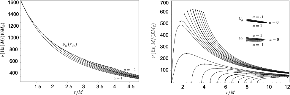 |
Figure 1:
Keplerian frequency |
| Open with DEXTER | |
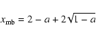
In the case of oscillating Keplerian discs three orbital frequencies are relevant:
Keplerian orbital frequency
![]() ,
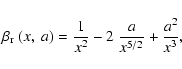
radial epicyclic frequency
,
radial epicyclic frequency
![]() =
=
![]() ,
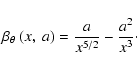
and vertical epicyclic frequency
,
and vertical epicyclic frequency
![]() =
=
![]() .
For discs orbiting Kerr black holes or naked singularities, corresponding angular velocities
.
For discs orbiting Kerr black holes or naked singularities, corresponding angular velocities
![]() ,
,
![]() ,
,
![]() are given by the well-known formulae (e.g., Nowak & Lehr 1999),
are given by the well-known formulae (e.g., Nowak & Lehr 1999),
| |
1-6 x-1+ 8 a x-3/2 -3 a2 x-2, | (4) | |
| 1-4 a x-3/2+3a2 x-2, | (5) |
In the limit of the Schwarzschild black holes (a=0), we arrive at
| (7) | |||
| (8) |
In the field of Kerr black holes (a ![]() 0), there is
0), there is
| (9) |
The properties of
![]()
![]()
![]() for Kerr black-hole spacetimes are rewieved, e.g., in Kato et al. (1998).
We can summarize that
for Kerr black-hole spacetimes are rewieved, e.g., in Kato et al. (1998).
We can summarize that
Obviously, all three frequencies (1)-(3) have the general form,
 |
(10) |
First, it is important to find the range of relevance for the functions
![]() ,
,
![]() ,
and
,
and
![]() above the event horizon located at
above the event horizon located at
 |
(11) |
| (12) |
![\begin{figure}
\par {\includegraphics[width=16.5cm]{2825_02.eps} }
\end{figure}](/articles/aa/full/2005/27/aa2825-05/img70.gif) |
Figure 2:
The locations
|
| Open with DEXTER | |
The circular geodesics in the field of Kerr black holes were discussed in Bardeen et al. (1972), while in the case of Kerr naked singularities the circular geodesics were discussed in Stuchlík (1980).
We can summarize that circular geodesics can exist in the range of
 |
(13) |
![\begin{displaymath}x_{\rm ph}~(a)=
2~
\left [
1+{\rm cos}
\left(
\frac{2}{3}~{\rm arccos}~(-a)
\right)~
\right ]
\end{displaymath}](/articles/aa/full/2005/27/aa2825-05/img72.gif) |
(14) |
| (15) |
| 1-6 x-1+ 8 a x-3/2 -3 a2 x-2=0, | (16) |
| (17) |
| (18) |
 |
(19) |
Clearly, the Keplerian orbital frequency is well defined up to x =
![]() .
However,
.
However,
![]() is well defined, if
is well defined, if
![]()
![]() 0, i.e., at x
0, i.e., at x ![]()
![]() ,
and
,
and
![]() = 0 at
= 0 at
![]() .
We can also show that for x
.
We can also show that for x ![]()
![]() ,
there is
,
there is
![]()
![]() 0; i.e., the vertical frequency
0; i.e., the vertical frequency
![]() is well defined at x >
is well defined at x >
![]() .
.
Denoting by
![]() ,
,
![]() ,
,
![]() the local extrema of Keplerian
the local extrema of Keplerian
![]() and epicyclic
and epicyclic
![]() ,
,
![]() frequencies, we can give the extrema by the condition
frequencies, we can give the extrema by the condition
 |
(24) |
 |
(25) |
![\begin{figure}
\par {\includegraphics[width=16.5cm]{2825_03.eps} }
\end{figure}](/articles/aa/full/2005/27/aa2825-05/img102.gif) |
Figure 3:
The locations
|
| Open with DEXTER | |
Relations (20) and (22) imply the condition determining extrema
![]() of the epicyclic frequencies:
of the epicyclic frequencies:
| (27) |
 |
(28) |
 |
(29) |
 |
(30) |
 |
(31) |
 |
(32) |
| (33) |
 |
(34) |
An example of the behaviour of the epicyclic frequencies in Kerr naked-singularity spacetimes is shown in Fig. 4 (right panel) for the case when all the local extrema mentioned above are present, while for an example of the case when the number of the local extrema is lowest see Fig. 9. The complete set of figures systematically representing the evolution of the character of the epicyclic frequencies with rotational parameter increasing is included in the Appendix which consists of Figs. A.1 (black holes) and A.2 (naked singularities); the evolution of derivatives (22) and of the ratio
![]() of the epicyclic frequencies is also included.
This set of figures represents classification of the Kerr spacetimes according to the properties of the epicyclic frequencies fully given in Sect. 5. Note that in the black-hole case it is important to distinguish the cases when the local maximum of
of the epicyclic frequencies is also included.
This set of figures represents classification of the Kerr spacetimes according to the properties of the epicyclic frequencies fully given in Sect. 5. Note that in the black-hole case it is important to distinguish the cases when the local maximum of
![]() is located above
is located above
![]() ,
and under
,
and under
![]() .
.
Clearly, the behaviour of the epicyclic frequencies substantially differs for Kerr naked singularities in comparison with Kerr black holes. We discuss some consequences of this different behaviour for naked singularities in Sect. 4, but first focus our attention on some properties of the epicyclic frequencies that are very important for treating the resonant oscillation phenomena from the observational point of view.
![\begin{figure}
\par {\includegraphics[width=16.5cm]{2825_04.eps} }
\end{figure}](/articles/aa/full/2005/27/aa2825-05/img123.gif) |
Figure 4:
Left panel: "unlikely" effects resulting from the existence maxima of
|
| Open with DEXTER | |
| |
Figure 5:
Left panel: the behaviour of ratio
|
| Open with DEXTER | |
The ratio of epicyclic frequencies
![]() and
and
![]() needs to be defined well for some models of QPOs (e.g., Kato 2004a; Abramowicz et al. 2004). It is well known (see, e.g., Kato et al. 1998) that for the Kerr black holes (
needs to be defined well for some models of QPOs (e.g., Kato 2004a; Abramowicz et al. 2004). It is well known (see, e.g., Kato et al. 1998) that for the Kerr black holes (
![]() )
the inequality
)
the inequality
| (35) |
| (36) |
 |
(37) |
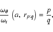
The orbital resonance models for QPOs proposed by Abramowicz & Kluzniak (Abramowicz et al. 2004; Abramowicz & Kluzniak 2001) are particularly based on resonance between epicyclic frequencies which are excited at a well defined resonance radius rp:q given by the condition
![\begin{figure}
\par {\includegraphics[width=16.5cm]{2825_06.eps} }
\end{figure}](/articles/aa/full/2005/27/aa2825-05/img132.gif) |
Figure 6: (After Kato et al. 1998) The simplest examples of wave propagation in a black-hole thin accretion disc: for fundamental axisymmetric mode (n=m=0) see left panel, while the first axisymmetric overtone (n = 1, m=0) is shown in the right one. Both figures are plotted for the Schwarzschild black hole. |
| Open with DEXTER | |
Indeed, this monotonicity of some resonant frequencies results from the nonmonotonic character of the epicyclic frequencies.
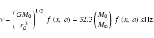
It is known that the radial epicyclic frequency has a local maximum at
![]()
![]()
![]() for
for
![]() and its value
and its value
![]() increases with the rotational parameter (see Fig. 1 - right panel). Moreover, outside its maxima it is monotonically decreasing with the radius. From the left panel of Fig. 5 we conclude that rp:q(a) must be a monotonically decreasing function of a. If the horizontal line representing some ratio p:q is fixed, then this figure implies a necessarily monotonically decreasing function
rp:q(a). Because of this, the resulting resonant frequency, which is just multiple of the radial frequency, must be monotonically increasing for rp:q located outside (or at) the maximum of the radial epicyclic frequency.
For Schwarzschild black holes the ratio between the epicyclic frequencies at the radius of maximal radial frequency is exactly
increases with the rotational parameter (see Fig. 1 - right panel). Moreover, outside its maxima it is monotonically decreasing with the radius. From the left panel of Fig. 5 we conclude that rp:q(a) must be a monotonically decreasing function of a. If the horizontal line representing some ratio p:q is fixed, then this figure implies a necessarily monotonically decreasing function
rp:q(a). Because of this, the resulting resonant frequency, which is just multiple of the radial frequency, must be monotonically increasing for rp:q located outside (or at) the maximum of the radial epicyclic frequency.
For Schwarzschild black holes the ratio between the epicyclic frequencies at the radius of maximal radial frequency is exactly
![]() = 2 (x = 8) and then changes slighty with the rotational parameter growing to reach the value
= 2 (x = 8) and then changes slighty with the rotational parameter growing to reach the value
![]()
![]() 1.8 for extremely rotating Kerr black hole (a = 1).
This gives the limit in the sense that for p:q > 1.8, the radius rp:q is certainly located above the maximum of
1.8 for extremely rotating Kerr black hole (a = 1).
This gives the limit in the sense that for p:q > 1.8, the radius rp:q is certainly located above the maximum of
![]() .
.
On the other hand, an analogical consideration shows that
![]() (or
(or
![]() ,
if the resonance condition (38) is satisfied) is surely decreasing with the rotational parameter, if rp:q is located under the location of the maximum of
,
if the resonance condition (38) is satisfied) is surely decreasing with the rotational parameter, if rp:q is located under the location of the maximum of
![]() .
The ratio of the epicyclic frequencies at the maximum of
.
The ratio of the epicyclic frequencies at the maximum of
![]() is shown in the middle panel of Fig. 5. Its minimum is reached for extremely rotating Kerr black holes at
is shown in the middle panel of Fig. 5. Its minimum is reached for extremely rotating Kerr black holes at
![]()
![]() 2.18. It means that for black holes the resonance is surely nonmonotonic if p/q
2.18. It means that for black holes the resonance is surely nonmonotonic if p/q ![]() 2.18.
2.18.
It is clear from the discussion above that the limit for nonmonotonicity must be located between the values of p/q![]() (1.8, 2.18). We numerically checked the loci of eventual nonmonotonicity and find that the limit is very close to the upper value; i.e., nonmonotonicity of the function
(1.8, 2.18). We numerically checked the loci of eventual nonmonotonicity and find that the limit is very close to the upper value; i.e., nonmonotonicity of the function
![]() in dependence on a is relevant for forced resonances with
in dependence on a is relevant for forced resonances with
| (39) |
Without going into detail, we explore simple examples to show that the physics of wave propagation and oscillations in thin accretion discs around the Kerr naked singularities is considerably different from the Kerr black hole case.
![\begin{figure}
\par {\includegraphics[width=16.5cm]{2825_07.eps} }
\end{figure}](/articles/aa/full/2005/27/aa2825-05/img144.gif) |
Figure 7:
The same examples of wave propagation as in Fig. 6, but for naked-singularity thin accretion disc (for the simplicity in degenerated case of a |
| Open with DEXTER | |
The systematic classification of oscillations and waves in accretion discs according to the restoring forces acting on them was summarized, e.g., in Kato et al. (1998). They introduced the following modes for disc oscillations:
We recall that the wave propagation is given by the dispersion relation (Nowak & Wagoner 1991; Kato 1989; Okazaki et al. 1987; Nowak & Wagoner 1992)
 |
(41) |
The overtones (![]() )
in Eq. (40) allow for the inertial acoustic p-waves, as well as inertial gravity g-waves. Generally, p-waves in this case must have frequency
)
in Eq. (40) allow for the inertial acoustic p-waves, as well as inertial gravity g-waves. Generally, p-waves in this case must have frequency ![]() >
>
![]() ,
while for g-waves the inequality
,
while for g-waves the inequality ![]() <
<
![]() must hold. The g-waves that could be trapped (see Fig. 6 - right panel) in the region around
must hold. The g-waves that could be trapped (see Fig. 6 - right panel) in the region around
![]()
![]()
![]() are insensitive to changes in disc structure, if the condition of a moderately geometrically thin disc is satisfied (Perez et al. 1997; Okazaki et al. 1987; Nowak & Wagoner 1992).
are insensitive to changes in disc structure, if the condition of a moderately geometrically thin disc is satisfied (Perez et al. 1997; Okazaki et al. 1987; Nowak & Wagoner 1992).
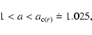
In the case of Kerr naked singularities, the well-known picture of the wave propagation, briefly recalled above, is changed due to the different behaviour of the epicyclic frequencies.
As shown in Sect. 3, the radial epicyclic frequency has two global maxima for Kerr naked singularities with
1 < a <
![]()
![]() 1.025.
Thus propagation of the fundamental axisymmetric (n = 0, m = 0)
1.025.
Thus propagation of the fundamental axisymmetric (n = 0, m = 0) ![]() -waves is changed (of course, the condition
-waves is changed (of course, the condition
![]() must be satisfied again):
must be satisfied again):
| |
Figure 8:
Left panel: the radial epicyclic frequency at particular extrema as a function of rotational parameter a between a = 1 and a = 1.025.
We can see that for a < 1.012 the global maximum is situated at
|
| Open with DEXTER | |
It is shown in Sect. 3 that for Kerr naked singularities with a >
![]()
![]() 1.089 the behaviour of epicyclic frequencies is formally similar to Kerr black holes.
However, for any naked singularity with
1.089 the behaviour of epicyclic frequencies is formally similar to Kerr black holes.
However, for any naked singularity with ![]() ,
the epicyclic frequencies (2, 3) can satisfy the equality condition
,
the epicyclic frequencies (2, 3) can satisfy the equality condition
| (42) |
Using the relation (43) in (2, 3) we find a strong resonant frequency that, in terms of the corresponding angular velocity, reads
 |
(44) |
 |
(45) |
![\begin{figure}
\par {\includegraphics[width=16.5cm]{2825_09.eps} }
\end{figure}](/articles/aa/full/2005/27/aa2825-05/img190.gif) |
Figure 9:
Left panel: behaviour of epicyclic frequencies for a = 2.3, the region where frequencies are identical with accuracy of 1%. The right panel illustrates the location of the strong resonant frequency (dotted curve a2) in relation to extrema of epicyclic frequencies (thin curve
|
| Open with DEXTER | |
The behaviour of the epicyclic frequency ratio
![]() typical of Kerr naked singularities is shown in Fig. 8 (middle panel).
In right panel in Fig. 8 we plot the value of the local extrema of the ratio
typical of Kerr naked singularities is shown in Fig. 8 (middle panel).
In right panel in Fig. 8 we plot the value of the local extrema of the ratio
![]() as a function of the rotational parameter a. For high values of the rotational parameter, the radial and vertical epicyclic frequencies are very close each other in large radial range around
as a function of the rotational parameter a. For high values of the rotational parameter, the radial and vertical epicyclic frequencies are very close each other in large radial range around
![]() .
This example is given in Fig. 9 (left panel).
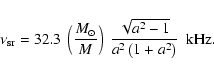
We plot the strong-resonance frequency as a function of the rotational parameter in Fig. 10 (left panel). It approaches zero value for an extremely rotating Kerr black hole and has a maximum for naked singularities with rotational parameter
.
This example is given in Fig. 9 (left panel).
We plot the strong-resonance frequency as a function of the rotational parameter in Fig. 10 (left panel). It approaches zero value for an extremely rotating Kerr black hole and has a maximum for naked singularities with rotational parameter
| (46) |
 |
(48) |
| (49) |
 |
(50) |
| |
Figure 10:
Left panel: the behaviour of strong resonant frequency shows remarkable maximum for the rotational parameter |
| Open with DEXTER | |
For Kerr naked singularities with any rotational parameter a, the ratio
![]() <
<
![]() being fixed can appear at three different radii. This kind of behaviour results from the existence of the strong resonance frequency (
being fixed can appear at three different radii. This kind of behaviour results from the existence of the strong resonance frequency (
![]() =
=
![]() )
for any Kerr naked singularity; i.e., it is not restricted to the cases when local extrema of
)
for any Kerr naked singularity; i.e., it is not restricted to the cases when local extrema of
![]() ,
,
![]() exist. This implies an important consequence for the resonant phenomena: in the case of slowly rotating Kerr naked singularities, an eventual resonance orbit rp:q (with p, q being small integral numbers) is defined ambiguously. In the range of frequencies
exist. This implies an important consequence for the resonant phenomena: in the case of slowly rotating Kerr naked singularities, an eventual resonance orbit rp:q (with p, q being small integral numbers) is defined ambiguously. In the range of frequencies
![]() ,
the resonant effects with the same rational ratio p:q can occur at three different radii rp:q.
Using the behaviour of the function
,
the resonant effects with the same rational ratio p:q can occur at three different radii rp:q.
Using the behaviour of the function
![]() (Fig. 8 - right panel) we can conclude that three radii rp:q could occur in the field of Kerr naked singularities with
(Fig. 8 - right panel) we can conclude that three radii rp:q could occur in the field of Kerr naked singularities with
![]() for p:q
for p:q ![]() :1,
:1,
![]() for p:q
for p:q ![]() :1, and
:1, and
![]() for p:q
for p:q ![]() :2.
:2.
The orbital resonance model (Kluzniak & Abramowicz 2002) demonstrates that fluid accretion flows admit two linear quasi-incompressible modes of oscillations, vertical and radial, with corresponding eigenfrequencies equal to vertical and radial epicyclic frequencies for free particles. In a particular model of slender torus, the general properties of these modes can be shown: the vertical mode corresponds to a periodic displacement in which the whole torus moves as a rigid body up and down the equatorial plane and each fluid element has a vertical velocity that periodically changes in time, but does not depend on the position. The frequency of the vertical mode is equal to the vertical epicyclic frequency that a ficticious free particle orbiting at the circle of maximum pressure in the torus equilibrium position would have. Behaviour of the radial mode is similar to the vertical one, and in the linear regime these two modes are formally uncoupled. Kluzniak & Abramowicz (2002) argue that in the case of more realistic description that includes non-linear effects given by pressure and dissipation, these effects couple the two epicyclic modes that may result in a resonance.
One possible resonance, the parametric resonance, seems to be the most probable explanation of the 3:2 double peak kHz QPOs observed in some galactic microquasars (Abramowicz et al. 2004). The effect itself is described by the Mathieu equation (Landau & Lifshitz 1976). After denoting the time derivative
![]() by dot
by dot
![\begin{displaymath}\delta \ddot \theta + \omega_{\theta}^2~[ 1 + h \cos~ (\omega_r t) ]~
\delta \theta = 0,
\end{displaymath}](/articles/aa/full/2005/27/aa2825-05/img214.gif) |
(51) |
| (52) |
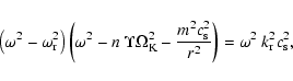
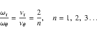
As shown above, the point where radial epicyclic frequency equals vertical epicyclic frequency exists for any Kerr naked singularity. Obviously, at such a point the equality (54) is satisfied (
![]() = 1/1 = 2/n; n = 2),
and the parametric resonance (between the radial and vertical epicyclic frequency) eventually excited at this point is the strongest possible parametric resonance excited between the epicyclic frequencies in the field of Kerr naked singularities. Such 2:2 resonance must also be stronger than the 3:2 parametric resonance in the black hole case (Landau & Lifshitz 1976).
= 1/1 = 2/n; n = 2),
and the parametric resonance (between the radial and vertical epicyclic frequency) eventually excited at this point is the strongest possible parametric resonance excited between the epicyclic frequencies in the field of Kerr naked singularities. Such 2:2 resonance must also be stronger than the 3:2 parametric resonance in the black hole case (Landau & Lifshitz 1976).
From this, and from the fact that the radial region with epicyclic frequencies that are nearly equal is rather large, one can expect that at this region both radial and vertical oscillations could be strongly amplified, leading to an instability of the accretion disc![]() .
.
For counterrotating Keplerian orbits, properties of the epicyclic frequencies are the same for all Kerr black holes and naked singularities. Radial epicyclic frequency always has a local maximum, while the vertical epicyclic frequency has no local extrema at x >
![]() .
.
On the other hand, for corotating Keplerian orbits, properties of the epicyclic frequencies strongly depend on the rotational parameter of the Kerr spacetimes. The most important difference between spacetimes with a < 1 and a > 1 is the change of inequality
| (55) |
In the case of Kerr black holes, the classification according to the properties of the epicyclic frequencies is given in the following way:
In the case of Kerr naked singularities, the classification is given as follows:
While wave propagation in the case of oscillations in the discs around Kerr naked singularities is substantially different from the black hole case only for spacetimes with
![]() ,
the strong resonance effect can occur for any Kerr naked singularity. The strong resonant frequency of disc oscillations around Kerr naked singularities always arise at the descending part of the function
,
the strong resonance effect can occur for any Kerr naked singularity. The strong resonant frequency of disc oscillations around Kerr naked singularities always arise at the descending part of the function
![]() ,
in the vicinity of the local minimum of
,
in the vicinity of the local minimum of
![]() ,
if this exists; i.e., it is always located above the innermost part of the disc. We stress that this phenomenon represents the strongest parametric resonance between the epicyclic frequencies possible in the field of Kerr naked singularities, stronger than in the case of Kerr black holes. Moreover, the area where the effect occurs is large which could have a strong influence on the stability of the Keplerian disc itself.
,
if this exists; i.e., it is always located above the innermost part of the disc. We stress that this phenomenon represents the strongest parametric resonance between the epicyclic frequencies possible in the field of Kerr naked singularities, stronger than in the case of Kerr black holes. Moreover, the area where the effect occurs is large which could have a strong influence on the stability of the Keplerian disc itself.
It follows from the existence of the strong resonant frequency that the function
![]() has the same character for all Kerr naked singularities with one local maximum
has the same character for all Kerr naked singularities with one local maximum
![]() > 1,
and one local minimum at
> 1,
and one local minimum at
![]() =
a2, a)=1 which corresponds to the strong resonant frequency. Because of this, some resonant effects can occur at three different radii rp:q with the same rational ratio p:q; i.e., resonant effects with the same ratios could be induced by very different physical phenomena at different parts of the accretion disc.
=
a2, a)=1 which corresponds to the strong resonant frequency. Because of this, some resonant effects can occur at three different radii rp:q with the same rational ratio p:q; i.e., resonant effects with the same ratios could be induced by very different physical phenomena at different parts of the accretion disc.
Finally we stress that the strong resonant frequency represents the phenomenon which we searched for in particular - i.e., the effect which could clearly indicate whether an observed X-ray is emitted from the accretion disc orbiting a naked singularity. If the resonant explanation of black-hole double peak QPOs is right, for naked singularities one can expect that the strong resonance 1:1 should significantly modulate in X-ray spectra one unique peak instead of two different peaks.
Acknowledgements
We thank Prof. Marek Abramowicz and Jirí Horák for discussions. This work was supported by the Czech grant MSM 4781305903. We also thank the perfect hospitality of Nordita (Copenhagen).
![$\displaystyle \phantom{-}\frac{3}{2}~\left[\frac{2~\beta_{{j}}}{\sqrt\alpha_{{j}}}-\frac{\sqrt{\alpha_{j}~x}}{\left({x}^{3
/2}+a\right)}\right]~\Omega_{\rm K},$](/articles/aa/full/2005/27/aa2825-05/img95.gif)
![\begin{figure}{\includegraphics[width=18cm]{2825_A1.eps} }
\end{figure}](/articles/aa/full/2005/27/aa2825-05/img244.gif)
![\begin{figure}{\includegraphics[width=17.8cm]{2825_A2.eps} }
\end{figure}](/articles/aa/full/2005/27/aa2825-05/img245.gif)