1 - Max-Planck-Institut für Astrophysik, Karl-Schwarzschild-Str 1, 85748 Garching bei München, Germany
2 - Department of Physics and Astronomy, University of Pittsburgh, 3941 O'Hara Street, Pittsburgh, PA 15260, USA
3 - Steward Observatory, University of Arizona, 933 North Cherry Avenue, Tucson, AZ 85721, USA

Abstract
We present first results on the quantitative spectroscopic analysis of the photospheric-phase of type II supernovae (SN). The analyses are based on the model atmosphere code, CMFGEN, of Hillier & Miller (1998) which solves the radiative transfer and statistical equilibrium equations in expanding outflows under the constraint of radiative equilibrium. A key asset of CMFGEN is its thorough treatment of line-blanketing due to metal species. From its applicability to hot star environments, the main modifications to the source code were to allow a linear velocity law, a power-law density distribution, an adaptive grid to handle the steep H recombination/ionization front occurring in some SN models, and a routine to compute the gray temperature structure in the presence of large velocities. In this first paper we demonstrate the ability of CMFGEN to reproduce, with a high level of accuracy, the UV and optical observations of a sample of well observed type II SN, i.e. SN1987A and SN1999em, at representative stages of their photospheric evolution. Two principal stages of SN are modeled - that where hydrogen is fully ionized, and that in which H is only partially ionized. For models with an effective temperature below $\sim$ 8000 K, hydrogen recombines and gives rise to a steep ionization front.

The effect of varying the location of the outer grid radius on the spectral energy distribution (SED) is investigated. We find that going to 5-6 times the optically-thick base radius is optimal, since above that, the model becomes prohibitively large, while below this, significant differences appear because of the reduced line-blanketing (which persists even far above the photosphere) and the truncation of line-formation regions. To constrain the metallicity and the reddening of SN, the UV spectral region of early-time spectra is essential. We find that the density of the photosphere and effect of line blanketing decline as the spatial scale of the SN increases. The density distribution is found to have a strong impact on the overall flux distribution as well as line profiles. For a given base density, the faster the density drops, the higher the effective temperature of the model. We also find in cool models that the set of Ca II lines, near 8500 Å is strongly sensitive to the density gradient. They show a weaker and narrower profile for steeper density distributions. Hydrogen Balmer lines are very well reproduced in fully or partially ionized models, but underestimated when hydrogen recombines. A reduced turbulent velocity or a flatter density layout are found to partially, but not fully, cure this persistent problem in studies of type II SN. He I lines observed in early-time spectra are very well reproduced, even for very modest helium enrichments, likely resulting from treatment of important non-LTE effects. At similar early epochs CMFGEN predicts, unambiguously, the presence of N II lines in the blue-wing of both H $\beta$ and He I 5875 Å. These lines have been observed but so far have generally been associated with peculiar emission, from locations far above the photosphere, in the strong adjacent lines.

Finally, we present a pedagogical investigation on P-Cygni profile formation in type II SN. H $\alpha$ is found to form very close to the photosphere and thus presents a significant flux-deficit in the red, made greater by the rapidly declining density distribution. This provides a clear explanation for the noticeable blue-shift of P-Cygni profiles observed in early-time spectra of type II SN.

Future studies based on CMFGEN modeling will focus on using type II SN for the calibration of distances in the Universe, as well as on detailed spectroscopic analyses for the determination of progenitor properties.

Key words: radiative transfer - stars: atmospheres - stars: supernovae - line: formation

1 Introduction

Following the development of radiative transfer algorithms suitable for expanding outflows (Mihalas et al. 1975), and advances in computer technology, increasingly detailed and successful quantitative spectroscopic analyses of massive stars and their winds have been carried out (cf., Schmutz 1997; Hillier & Miller 1998, 1999; Hamann & Koesterke 1998). Such quantitative spectroscopic studies can shed light on numerous properties of optically-thick outflows, with implications for understanding the parent object. One can determine the chemical composition, radius, luminosity, density, ionization structure and kinematic properties of the star and its wind, as well as the temperature of the equivalent blackbody at the thermalisation depth.

Although stellar winds are radiatively-driven, the mechanisms controlling the escape of photons from the optically-thick flow are similar in nature to that occurring in the freely-expanding fast ejecta associated with supernovae (SN) explosions, occurring either via core-collapse of a massive star (H-free type Ib/c or H-rich type II; Arnett et al. 1989) or thermonuclear runaway of a Chandrasekhar mass white-dwarf (type Ia; Hillebrandt & Niemeyer 2000). In the context of SN, spectroscopic modeling allows inferences on the properties of the progenitor of the explosion to be made, providing clues to the evolution and death of stars, as well as the formation of compact objects.

Additionally, massive stars, and SN explosions to a much larger extent, are so intrinsically luminous that attempts to use them as distance calibrators have been made. For example, massive stars can be used to constrain the Hubble constant via the Wind-Momentum-Luminosity relation (Kudritzki et al. 1999). Light curves of type Ia SN have been used to claim that we live in an accelerating universe (Riess et al. 1998). Finally, although type II SN are not as bright as type Ia events, they can be used with variations on the Baade's method (Baade 1926), i.e. the Expanding Photosphere Method (EPM; Kirshner & Khan 1974; Eastman & Kirshner 1989; Eastman et al. 1996; Schmidt et al. 1994a,b; Leonard et al. 2002a,b; Hamuy & Pinto 2002) and the Spectral-fitting Expanding Atmosphere Method (SEAM; Baron et al. 1995, 2004), to provide distance estimates for objects even within the Hubble flow. However, such distance determinations will benefit from a thorough modeling of the SN spectrum and light curve, as well as from an understanding of the physics of spectrum formation.

Model atmospheres and techniques, which have been tested so heavily and applied so successfully to hot luminous stars, constitute excellent tools for such SN analyses. This is being done with a number of codes: WM-BASIC (Pauldrach et al. 2001, 1996) PHOENIX (Hauschildt 1992a,b; Hauschildt & Baron 1995), EDDINGTON (Eastman & Pinto 1993). Our analyses are based on CMFGEN (Hillier & Miller 1998), which has been used to model OB stars, Luminous Blue Variables (LBVs) and Wolf-Rayet (WR) stars (Hillier et al. 1998; Dessart et al. 2000; Crowther et al. 2002; Hillier et al. 2003).

O star winds are weak and scattering dominated, quite like SN outflows. In the weakest-wind O-stars, line formation occurs over a small spatial region so that sphericity effects are unimportant. On the contrary O-supergiants, where sphericity effects are important, show a range of line formation processes, with both photospheric and wind sites of emission, absorption and scattering (Hillier et al. 2003; Martins et al. 2004; Crowther et al. 2002). Conversely, LBV winds are very extended, dense and relatively cool, and have an ionization structure that resembles quite closely that of SN. Processes such as Rayleigh scattering, charge exchange and two-photon decay are of relevance in both LBV and SN outflows (Hillier et al. 1998, 2001; Najarro et al. 1997). WR winds are dense and fast, and typically show a much higher ionization than SN. Their composition is typical of progenitors of type II (H-rich) and type Ib/c (H-free) SN (Dessart et al. 2000; Crowther et al. 2002).

Despite the similarities, SN conditions depart from those of hot star winds in a number of ways. The flow is accelerated only temporarily, say for about a day after core-collapse or explosion, followed by a homologous expansion in which the velocity follows a Hubble law (v/r constant - Woosley 1988). Consequently the outflow density profile does not follow an inverse square law as imposed by mass conservation (Castor et al. 1975), but instead results from the disruption of the envelope by the shock wave arising from the explosion (Woosley 1988). Indeed models of such explosions, as well as spectroscopic analyses, support a very fast decreasing density. This rapid density decline, together with the large velocity gradient, are key ingredients controlling the escape of radiation from the flow.

Another key component for the modeling of outflows is the origin of opacity. In H-rich environments, such as massive star winds and type II SN, the dominant source of continuum opacity is electron scattering. Although electron scattering is more important in type II SN, there is still significant true absorption, due to bound-free and free-free processes, to allow the diffusion approximation, and the assumption of LTE, to be applied at the base of the outflow. For H-free conditions, bound-free and bound-bound transitions of metals will become the dominant source of opacity. There, including as many levels and lines is mandatory for recovering LTE and a thermalisation layer at the base.

Because of their closer similarity to hot massive stars, we concentrate on type II SN in this first series of papers. In this first paper, we present the necessary adjustments made to CMFGEN in order to model the emergent spectra from SN outflows, and provide some key insights into SN spectrum formation. In Sect. 2, we present the code of Hillier & Miller (1998), giving the necessary background and highlighting key differences between CMFGEN and other models developed and used by different groups. We also describe the adjustments from hot star to SN conditions. In Sect. 3, we present typical results of our spectroscopic modeling, selecting a sequence of observations taken during the photospheric-phase evolution of SN1987A and SN1999em. These serve as illustrations for the model behavior, as well as a basis for our interpretation of key features of type II SN during the photospheric phase. We also give model parameters, discuss outflow properties and provide line identifications. In Sect. 4, based on the models shown in Sect. 3 as well as the large parameter space investigated for the preparation of this paper, we describe generic features of type II SN and how these are sensitive to model parameters. We discuss the handling of the H-recombination front in cool models (Sect. 4.1), the potential problem with the choice of outer grid location (Sect. 4.2), the importance of line-blanketing (Sect. 4.3), the influence of the luminosity (Sect. 4.4) and density exponent (Sect. 4.5) on the spectral morphology, and the modeling of hydrogen, helium and nitrogen line profiles in the optical range (Sect. 4.6). In Sect. 5, we describe in detail the process of line formation in type II SN, giving in particular a physical explanation for the observed blue-shift of Balmer lines in photospheric-phase spectra of type II SN. In Sect. 6, we present our conclusions and map out our future endeavors.

2 Presentation of the code

Our effort to analyze the light emanating from SN outflows makes use of the model atmosphere code CMFGEN, discussed in detail by Hillier & Miller (1998, 1999). CMFGEN solves the radiative transfer equation in the comoving frame, subject to the constraints of radiative and statistical equilibrium. The outflow is assumed to be steady-state and to have a spherical symmetry. The general procedure for analyzing a given object is to input global characteristic quantities such as luminosity, radius, chemical composition, velocity and density.

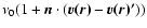
In hot star outflows, the velocity law is taken from detailed hydrodynamical computations of radiatively-driven winds. For SN outflows, after about one day after the explosion, the outflow no longer accelerates but instead freely-expands into the surrounding medium. Such an homologous expansion is characterized by a Hubble velocity law, v(r) = v₀ (r/R₀)where R₀ is the base radius where the luminosity is input, and v₀ the velocity of this layer. This layer in type II SN is chosen such that it is optically thick at all wavelengths and thus corresponds to a thermalisation layer where photons have a Planckian distribution at the local temperature $T= (L_{\ast}/4 \pi \sigma R_0^2)^{1/4}$ , $\sigma$ being Stefan's constant. Note that this lies significantly below the photosphere which we define as the layer where the total continuum optical-depth is 2/3 (this includes bound-free and free-free processes from all species plus electron-scattering), located typically around 1.3-1.5 R₀. As time proceeds, (constant-velocity) mass shells expand and become more optically thin, so that in the frame comoving with a given mass shell, the thermalisation layer recedes deeper into the flow. At present, the time evolution is taken into account by fitting not only the spectral energy distribution (SED) but also the absolute flux level at all times. The former gives a tight constraint on the ionization balance of the flow and the temperature of the thermalisation layer. The second constrains the luminosity (or radius of the thermalisation layer). In practice, we vary the outflow ionization and the absolute flux level by adjusting the radius scale of the model, controlled by the parameter R₀, and the luminosity (or the flux) going through this inner model boundary, controlled by the parameter $L_{\ast}$ .

For the distance, which is required for the luminosity constraint, we have adopted the Cepheid or EPM distance to the object under investigation. As discussed later in this paper, for a given outflow ionization, the SED is only sensitive to large changes in luminosity so uncertainties in the distance, at the 50% level, will have negligible effects on the SED.

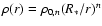
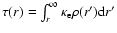
We adopt an analytical density law and adjust it at different epochs according to whatever nature demands. Later we show that the steepness of the density fall-off is mostly constrained by P-Cygni line profile shapes. The analytical form adopted is a power law, i.e. $\rho(r) = \rho_0 (R_0/r)^n$ . Former investigations, both of the explosion itself as well as others on the SED have shown that n is large, with a nominal value of 10, and tends to decrease over time (see, e.g., Arnett 1988; Lucy 1987; Eastman & Kirshner 1989). $\rho_0$ is adjusted so that the Rosseland-mean or electron-scattering optical depth at the base is of the order of 50. This ensures photons are thermalised in the base layer.

In radiatively-driven winds of hot stars, the density is usually taken to be clumped on small scales since this is expected both theoretically (Owocki & Rybicki 1984; Dessart & Owocki 2003) and observationally (Robert 1992). In multi-dimensional simulations of SN explosions (Kifonidis et al. 2003; Reinecke et al. 2002), density contrasts in the heterogeneous outflows are of the order of a few at most, thus more than an order of magnitude less than suspected in hot stars. Hence, we assume no clumping of the outflow in our simulations. As we show in the next section, the quality of the fits is excellent, suggesting that clumping, if present, remains small.

In addition to clumping, SN outflows are expected to exhibit turbulence on a variety of scales (see, e.g., Kifonidis et al. 2003; Burrows et al. 1995). We generally adopt a microturbulent velocity of 100 km s^-1, which is just a few percent of the photospheric velocity - this has the effect of broadening the intrinsic (Gaussian) line profile width, increasing the probability of line-overlap but reducing the required frequency sampling for the radiative-transfer solution. Large scale turbulent motions are ignored.

In type II SN, only a small amount of metals is nucleo-synthesized during the explosion (Woosley & Weaver 1995), so that it seems suitable to assume strict radiative-equilibrium. To ensure that such a situation prevails, we limit our investigation to early times during the photospheric phase, say the first month after maximum B band light.

A key asset of CMFGEN is that all lines of all species are treated in non-LTE. Since adequate modeling of the blanketing effects of iron are essential, and since such a metal has a very complex atomic structures with lots of lines, the atomic structure input in the code is re-organized in terms of "super-levels'' (SL). In this scheme nearby levels, having similar departure coefficients, are grouped together and treated as an individual level. Despite this grouping, all lines are treated at their correct wavelengths (ignoring possible difficulties with the atomic data). Applying this procedure to all species permits the treatment of many more ions and bound-bound transitions. In our approach we do not need to assign an absorption/scattering cross section to the line blanketing. This is automatically determined by the coupled solution of the transfer and statistical equilibrium processes. If the SL assignment is too coarse, branching (i.e., the decay of the upper level to alternate states) may not be treated correctly. In particular, to treat the Bowen fluorescence mechanism, special care must be taken when making the SL assignments. However, numerous tests, in a wide variety of conditions, have shown that the SL approach can yield an accurate temperature and ionization structure of the envelope. Importantly, it is relatively easy to change the SL assignments to test their effect.

We show in Table 1 the largest atomic model used in our computations, showing the number of "full-'' and "super-'' levels, and the corresponding number of transitions. For coarse analyses, only H, He, C, N, O and Fe are included. In fact, including Fe II ensures that the overall temperature structure and ionizing flux are not significantly affected when performing the more detailed computation with the larger model atom. The atomic data come from a wide variety of sources, the Opacity Project (Seaton 1987; The Opacity Project Team 1995, 1997), the Iron Project (Pradhan et al. 1996; Hummer et al. 1993), Kurucz (1995), and the Atomic Spectra Database at NIST Physical Laboratory being the principal sources. Much of the Kurucz data was obtained directly from the Center for Astrophsyics (Kurucz 1988, 2002). Individual sources of atomic data include the following: Bautista & Pradhan (1997), Becker & Butler (1995), Butler et al. (1993), Fuhr et al. (1988), Kingdon & Ferland (1996), Luo & Pradhan (1989), Luo et al. (1989), Mendoza (1983), Mendoza et al. (1995), Nahar (1995, 1996), Nahar & Pradhan (1996), Neufeld & Dalgarno (1987), Nussbaumer & Storey (1983, 1984), Peach et al. (1988), Storey (1988), Tully et al. (1990), Wiese et al. (1966), Wiese et al. (1969), Zhang & Pradhan (1995, 1997). Note that at present, we are missing some species for the modeling of late-stage spectra, most importantly C I, Sc II and Ba II, something we will remedy in the future.

Table 1: Summary of the model atom used in our calculations. $N_{\hbox {\sc f}}$ is the number of full levels, $N_{\hbox {\sc s}}$ the number of super levels and $N_{\hbox {\sc t}}$ the corresponding number of transitions.

Before describing results obtained with CMFGEN, it is worthwhile stressing the differences with other models used for SN studies. As described in the introduction, a number of general purpose model atmosphere codes, often developed originally for the treatment of the expanding outflows of hot stars, have been applied to SN. The general practice for the study of type II SN is to assume spherical symmetry and steady-state, although some attempts are now made to perform 3D Monte-Carlo radiative-transfer calculations (Thomas et al. 2003). The level of refinement for the radiative transfer computation varies significantly: many studies treat all metal lines in LTE, using non-LTE for H and He only (Schmutz et al. 1990; Eastman et al. 1989, 1996). Although much more computationally expensive, a higher level of consistency is met by studies that treat instead all lines in non-LTE (Höflich 1988; Mitchell et al. 2002). Finally, the alternative parameterized approach with SYNOW, tagged "direct-analysis'', is less physically consistent than previous methods, but constitutes a useful tool to identify spectral features - a challenging task in SN spectroscopy - and can thus serve as a basis for more accurate model atmosphere computations.

Before proceeding further it is worth giving an honest appraisal of some of the deficiencies of the present study. First we assume spherical geometry and homogeneity. Many spectropolarimetric studies have shown that at least for some SN, a departure from spherical symmetry on a large scale is present, although mostly restricted to late times (see, e.g., Kasen et al. 2003, for type Ia SN, Höflich et al. 1996, for type Ib SN, and Leonard et al. 2001, for type II SN). Further, due to Rayleigh-Taylor instabilities, there is likely to be substantial mixing of material from the inner layers into the outer layers (Kifonidis et al. 2003), as well as smaller scale structures (with a scale of the order of or below the photospheric radius value). One such evidence for inhomogeneities was seen in H $\alpha$ line profile variations in late-time spectra of SN 1987A (Spyromilio et al. 2003). Second, we neglect the time dependence of the flow. This is certainly not valid for modeling the luminosity evolution from hydrodynamical calculations, especially at early times, but is expected to be a reasonable approximation in the atmosphere where we can fix the luminosity using observations.

At present we ignore relativistic effects other than the frequency shift arising from the first order Doppler correction. Such effects have been discussed by Hauschildt et al. (1991), and will be the subject of another paper. All these effects are crucial for hydrodynamical modeling, but less so in the approach we adopt where we constrain the emitted luminosity by the observations, and only treat the "photospheric'' layers. Other effects, such as an accurate treatment of line blanketing, are much more important in determining the observed spectrum. The primary motivation for doing so was to utilize CMFGEN in a standard configuration - this allowed convergence difficulties to be attributable to the properties of SN envelopes, rather than complications arising from the relativistic transfer. In an earlier attempt at modeling SN the strongly scattering envelope gave rise to difficulties in the temperature convergence which were wrongly attributed to problems in the relativistic transfer, whereas they were related to the use of SL (Hillier 2003).

Due to the large photospheric velocities, we modified the gray temperature formulation to take into account the first order Doppler shifts. This formulation was necessary to provide an improved estimate of the temperature structure at depth at the beginning of the model iteration.

3 Spectroscopic modeling

In the present paper, we wish to discuss the basic properties of a few models whose synthetic spectrum fits reasonably well the observations at early, intermediate and late times of the photospheric-phase evolution of type II SN. We base our discussion on two very well observed type II SN, SN1987A and SN1999em. The former was associated with the neutrino detection on February 23.316 UT 1987 with the Kamiokande detector (Koshiba 1987). Here, we use the first spectrum taken both in the UV and in the optical (Pun et al. 1995; Phillips et al. 1988), on February 24th, thus only one day after discovery (and collapse). We use this observation for the early-stage description of type II SN spectra. For SN1999em, no neutrino detection was made and thus no precise dating of the core-collapse of the progenitor exists. Inferences, based on the light curve appearance or the EPM, suggest the explosion took place at around October 27th 1999, with an uncertainty of 1-2 days. It was absent in images of the host galaxy NGC 1637 taken on October 20.45 UT, while first detection of the SN was made on October 29th (JD 2451480.94; Li 1999). The resemblance of the spectrum taken on October 30th with the spectrum of SN1987A taken on the 24th of February 1987, indicate that SN1999em was indeed caught at a very early phase of evolution. Here, we use observations of SN1999em taken on the 5th of November 1999 (ca. one week after explosion; Baron et al. 2000; Leonard et al. 2002a) and on the 14th of November 1999 (ca. two weeks after explosion; Hamuy et al. 2001) to describe respectively the typical intermediate- and late-stage appearance of type II SN spectra. Such time qualifications to observations are to be taken in a broad context. We defer until a follow-up paper a detailed analysis with a fine time-sampling of the evolution of the SED of a type II SN during the entire photospheric phase.

Let us describe the spectral evolution in the UV/optical ranges of these two well observed SN. For each SN, the first spectrum taken shares striking similarities: the flux in the UV is much larger than in the optical where one sees hydrogen Balmer lines and He I 5875 Å. Following this stage, as the outflow expands and cools, the UV flux diminishes and the He I 5875 Å P-Cygni profile weakens. Depending on the object, this takes a range of time scales: SN1987A did that step in just one day, while the corresponding spectral evolution took 10 days for SN1999em. One can then identify a cooler stage where both the UV flux and He I lines are completely gone. Metal lines start appearing in the optical range and the Ca II multiplet around 8500 Å is present. Further, the Na I doublet at 5890 Å starts appearing as a weak P-Cygni profile. During this entire sequence of events, hydrogen recombination becomes more and more pronounced so that the next stage is characterized by the presence of the hydrogen recombination front close to the photosphere. The SED (i.e., $f_\lambda$ ) then peaks at or beyond 4000 Å. Subsequent evolution is more gradual, with significant changes taking place over longer time-scales.

When fitting synthetic spectra to observations, we redden the theoretical SED using the Cardelli law (Cardelli et al. 1988) for SN1999em and the Seaton (1979) and Howarth (1983) laws for the Galaxy and the LMC respectively. For SN1987A, we take the Cepheid distance to the LMC of 52 kpc for SN1987A and adopt a reddening value E(B-V)=0.05 for both galactic and LMC components. This is slightly less than the value 0.16 proposed by Lundqvist & Fransson (1996) but seems warranted to reproduce the observations of SN1987A on the 24th of February. For later times, this choice has essentially no effect on the fit quality to observations. For SN1999em, we use the Cepheid-based distance of 11.7 Mpc to NGC 1637, somewhat different from the EPM based distance of 8.2 Mpc (Leonard et al. 2002a) or 7.5 Mpc (Hamuy et al. 2001). These differ slightly but within such limits, the computed SED remains identical, only the absolute flux level to reproduce observations will change, by about a factor of two. Note finally that we correct for the recession velocity of the galaxy host of SN1999em by blue-shifting the observations by 770 km s^-1 (Leonard et al. 2002a; Baron et al. 2000).

Due to the ubiquitous presence of line-overlap, it is instructive to investigate which lines contribute to observed "line features''. Except on very rare occasions and/or for very few lines (early-spectra in the optical, H $\alpha$ for most epochs), the very large expansion velocities are such that observed features are composed of different lines of different species. If these arise from species with differing ionization potential, they are likely to form in distinct regions of the outflow and therefore have a profile width and strength quite unpredictable a priori. To assess the importance of this issue, our code can compute the emergent spectrum from a formal solution of the transfer equation based on the full non-LTE solution, including all continuum processes (all bound-free and free-free processes) but including only the line transitions of the desired species/ionization stage. Although this then ignores the non-linear interaction of overlapping lines on the observed spectrum, it allows us to assess with enough accuracy what species contribute to a given feature.

Finally, in each of the following sections, we give details on model parameters corresponding to the synthetic spectra shown in the figures. However, unless otherwise stated, all simulations use a chemical composition adequate for a young supergiant massive star. In practice, we use the following CNO-cycle equilibrium values for a massive progenitor star (Prantzos et al. 1986): slightly enriched abundances of helium and nitrogen ${\rm H/He}=5$ , ${\rm N/He} = 6.8 \times 10^{-3}$ , and depletion of C and O, i.e. ${\rm C/He} = 1.7 \times 10^{-4}$ and ${\rm O/He} = 10^{-4}$ (all given by number). Additionally, when the model refers to SN1999em, the abundance of metal species (excluding CNO elements) is set to its Solar Neighborhood value. This is compatible with the inferred solar or over-solar metallicity of its host galaxy NGC 1637 (Leonard et al. 2002a). For SN1987A, metal abundances are all scaled by a fixed factor of 0.4, compared to their solar value.

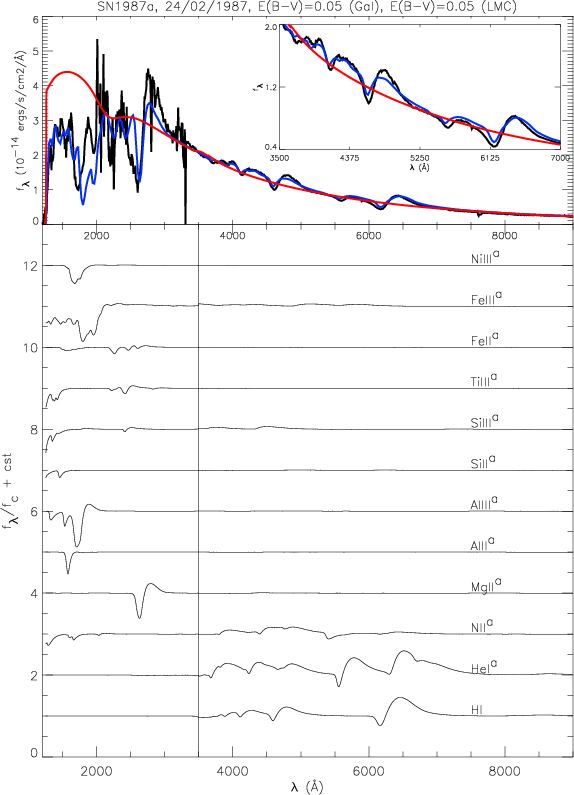
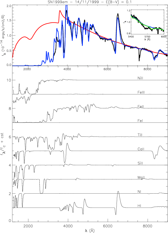
3.1 Early stage

We show in the top panel of Fig. 1 synthetic fit (color) to observations (black) of SN1987A taken on the 24th of February 1987. The red curve represents the continuum energy distribution of the model, while the blue curve corresponds to the synthetic flux distribution when all line and continuum processes are included.

$\begin{figure} \par\epsfig{file=2525f1.eps, width=8.8cm,clip}\end{figure}$

Figure 1: Top: illustration showing the comparison between reddened model spectra (blue) and observations of SN1987A (black) taken on the 24th of February 1987 (Pun et al. 1995; Phillips et al. 1988). Each model flux distribution is scaled for an assumed LMC distance of 52 kpc. In red we show the theoretical continuum energy distribution of the model. Model characteristics are: $L_{\ast} = 3 \times 10^8~L_{\odot}$ , $R_{\rm phot} = 2.74 \times 10^{14}$ cm (or 3940 $R_{\odot }$ ), $v_{\rm phot}=17~700$ km s^-1, $T_{\rm eff} =11~200$ K, n=12, $\rho _{\rm phot} = 1.1 \times 10^{-13}$ g cm^-3. Bottom: montage of rectified spectra computed by including bound-bound transitions of individual species, ordered from the bottom by increasing atomic weight. For species labeled with an "a'', we show $(f_{\lambda }/f_{\rm c}-1) \times x{\rm scale}+1$ , with $x{\rm scale}=4$ beyond 3500 Å and unity elsewhere [color].

Open with DEXTER

The outflow ionization is high with a SED that peaks in the UV. The line-blanketing due to metal species is modest - a significant UV flux is still present. We show in the bottom panel of Fig. 1 the actual contribution from each of the species present, by computing the synthetic spectrum including only the bound-bound transitions of a given species. The resulting SED is then normalized by the continuum energy distribution and ordered in Fig. 1 by increasing atomic weight, starting from the bottom. To enhance the visibility of weak optical features, that nonetheless contribute to observed features, we apply a scaling to the rectified spectra so that we in fact show $(f_{\lambda }/f_{\rm c}-1) \times x{\rm scale}+1$ , with $x{\rm scale}=4$ beyond 3500 Å, and unity elsewhere.

Few features are actually associated with a small set of lines. At 2800 Å, the feature is due to Mg II(3p-2s) 2802.7 Å and the doublet Mg II(4s-3p) 2928.6-2936.5 Å. At 1900 Å, the feature is due to a small but larger number of Al III lines, predominantly Al III(3p-3s) 1859 Å and (4f-3d) 1935 Å. Other UV features are the result of a large number of lines, in particular from Fe III and Ni III. Indeed, the combination of a rich line-spectrum of metals, particularly that of iron, together with the large Doppler shifts induce a strong line-blocking effect on the radiation field.

In the optical (see the inserted zoom in the top right corner of Fig. 1), we find the usual suspects of type II SN, i.e. hydrogen Balmer lines: H $\alpha$ at 6562.8 Å, H $\beta$ at 4861.3 Å, H $\gamma$ at 4340.5 Å, H $\delta$ at 4101.7 Å, and H $\epsilon$ at 3970.0 Å. At shorter wavelengths, the higher transitions in the Balmer series merge together until the Balmer jump at 3646 Å. The later region might be weakly contaminated by the presence of the Ca II doublet (4p-4s) at 3933.6-3968.5 Å.

We can also find the presence of the He I 5875 Å. For SN1987A, this line is only present in the first spectrum, shown here, while for SN1999em, this line is observed for about a week (see Sect. 4.6.2). It serves as a key diagnostic of the outflow ionization since for just slightly cooler temperatures, it becomes optically-thin and its strength vanishingly small. He I 5875 Å is the one helium line that gets most attention because it is isolated and thus, uncontaminated. However, the model predicts the presence of a group of He I lines around 4000 Å (He I(3p-2s) 3888.6 Å, He I(4p-2s) 3964.7 Å, He I(7d-2p) 4009.2 Å, He I(7s-2p) 4024.0 Å, He I(5d-2p) 4026.2 Å ) as well as around 4500 Å (He I(5d-2p) 4388.1 Å, He I(5s-2p) 4437.5 Å, He I(4d-2p) 4471.5 Å, He I(4s-2p) 4713.1 Å), followed by He I(4d-2p) 4921.9 Å and He I(3d-2p) 6678 Å. The strength of the resulting features is predicted to be of the same order as that of He I 5875 Å and hence, it is clear that helium lines are present throughout the optical range.

We also find the presence of N II lines in the optical: in the blue wing of He I 5875 Å as well as in the blue wing of H $\beta$ , at respective wavelengths of 5495-5680 Å and 4477-4630 Å (each of these is part of a multiplet). In SN1987A, these features are quite weak (resulting to a large extent from its unusually high expansion velocity) but their unambiguous presence is seen in the early spectra of SN1999em (see Sect. 4.6.3) and even more so in SN1999gi (Leonard et al. 2002b). We defer until Sect. 4.6.3 for a more detailed discussion on these N II lines and their presence in early spectra of type II SN. For carbon and oxygen, their expected under-abundance during the CNO cycle due to mass loss (Prantzos et al. 1986), which we adopt here, is such that not a single line from C II, C III, O I, O II, O III is predicted to be noticeable in this model. Note also that one can see few weak features arising from Si III and Fe III lines in the optical, while most metal features are in the UV at this epoch.

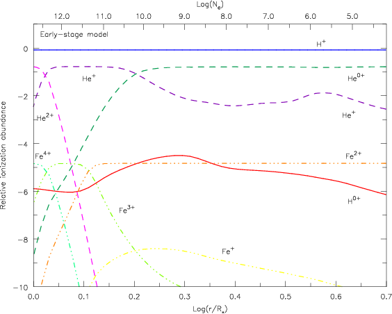
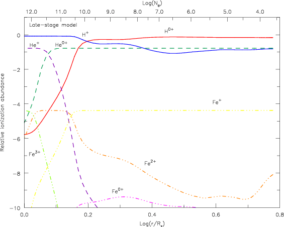
Finally, we display the outflow ionization in Fig. 2. Hydrogen is fully ionized, helium doubly ionized only at the base, singly ionized at intermediate heights and neutral in the outer part of the outflow. Iron is present in the form of Fe⁴⁺ inside through to Fe²⁺ outside, with Fe⁺ never setting in. Note that in this model, the photosphere is located at r=1.48 R₀ or $\log(r/R_0) = 0.17$ , thus in a region where H⁺, He⁺ and Fe²⁺ dominate.

$\begin{figure} \par\epsfig{file=2525f2.eps,angle=-90,width=8cm,clip}\end{figure}$	Figure 2: Relative ionization for hydrogen (solid), helium (dashed) and iron (dash-dotted line) for the early-stage model of Sect. 3.1 and Fig. 1. The ionization fractions are expressed relative to the abundance of all species. Also shown is the electron density on the top axis [color].
Open with DEXTER

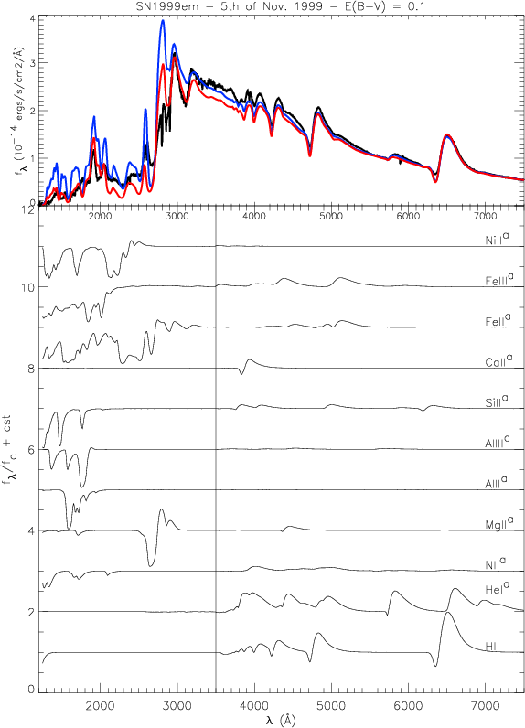
3.2 Intermediate stage

In this and the following section, we turn to the subsequent evolution of type II SN spectra, using observations performed at ca. 1 and 2 weeks after the estimated explosion time of SN1999em (Li 1999; see introduction to Sect. 3).

We show in Fig. 3 synthetic fits (color) to observations (black) taken on the 5th of November by Baron et al. (2000) using the Hubble Space Telescope, as well as optical observations from Leonard et al. (2002a). The two models differ only in luminosity: $L_{\ast} = 4 \times 10^8~L_{\odot}$ for the red model and $L_{\ast} = 5 \times 10^8~L_{\odot}$ for the blue model. The resulting model properties differ only in effective temperature: $T_{\rm eff} = 8850$ K (red model) and $T_{\rm eff} = 9200$ K (blue model) while the common properties (parameters) are the following: $R_{\rm phot} = 6.6 \times 10^{14}$ cm (or 9540 $R_{\odot }$ ), $v_{\rm phot}=8750$ km s^-1, n=10 and $\rho _{\rm phot} = 4.1 \times 10^{-14}$ g cm^-3. The red model would give a better fit to observations if we chose E(B-V)= 0.08-0.09 instead of the adopted value of 0.1. This shows that the UV range is important to place very strong constraints on the model temperature as well as the adopted reddening, helping to lift the degeneracy in the impact of these two parameters.

$\begin{figure} \par\epsfig{file=2525f3.eps, width=8.8cm,clip}\end{figure}$

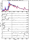Figure 3: Top panel: synthetic fit (color) to HST and Lick observations (black) of SN1999em taken on the 5th of November 1999 (Baron et al. 2000; Leonard et al. 2002a). The red (blue) curve corresponds to a model with $L_{\ast} = 4 \times 10^8~L_{\odot}$ ( $L_{\ast} = 5 \times 10^8~L_{\odot}$ ) and $T_{\rm eff} = 8850$ K ( $T_{\rm eff} = 9200$ K). Other properties are identical: $R_{\rm phot} = 6.6 \times 10^{14}$ cm (or 9540 $R_{\odot }$ ), $v_{\rm phot}=8750$ km s^-1, n=10 and $\rho _{\rm phot} = 4.1 \times 10^{-14}$ g cm^-3. Lower panel: montage of rectified spectra (same as in Fig. 1) [color].

Open with DEXTER

In the bottom panel of Fig. 3, we show the synthetic spectrum for the blue model when only the bound-bound transitions of selected species (indicated on the right) are included together with all bound-free and free-free processes. As in Fig. 1, we apply a scaling of a factor of four to the rectified spectra beyond 3500 Å to enhance the visibility of weak features.

At this stage of its evolution, the SN outflow has cooled significantly, so that Fe II line-blanketing starts to strongly diminish the UV flux. This blanketing is not so severe, so that some residual UV flux is observable, carrying information on the species at its origin. From the lower panel, we see that the line-blanketing makes the UV flux smaller than the continuum flux when all lines are ignored. In other words, emission features in the UV are to be understood as spectral windows where this line-blanketing is less relative to nearby regions, rather than an excess flux above the continuum level. We thus identify enhanced line-blocking due to Fe II, Fe III, Ni II, Si II, Al II, Al III. An exception to this is due to Mg II lines, already discussed in the previous section, which show pronounced emission and absorption around 2800 Å.

In the optical range, besides hydrogen lines, He I features are numerous with a strength of about one fifth of H $\alpha$ (see previous section for a census of these lines). However, the outflow has cooled down too significantly to show N II lines, and we instead see the appearance of weak metal lines in the optical spectrum. We have the Mg II(4f-3d) triplet at 4481 Å. We also have Si II(5p-3d)4076.8, Si II(4f-3d) 4128.0 Å, the Si II(4d-4p) doublet at 5056.0 Å and the Si II(4p-4s) doublet at 6347.1 Å and 6371.4 Å. We finally attribute some features to Fe II and Fe III but due to the large number of contributors, we cannot enumerate them. Note nonetheless that contrary to identifications by Leonard et al. (2002a), the feature around 5200 Å has Fe III lines (groups of lines around 5080 Å and 5160 Å) as main contributors, rather than Fe II, and also overlaps with lines of Si II at 5056 Å and He I at 4921.9 Å and H $\beta$ . This careful log shows that it is difficult to associate "features'' in SN spectra with individual lines of selected species.

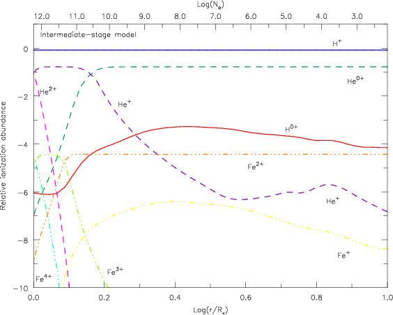
$\begin{figure} \par\epsfig{file=2525f4.eps, angle=-90, width=8cm,clip}\end{figure}$	Figure 4: Ionization structure for the intermediate-stage model described in Sect. 3.2 and shown in Fig. 3. The ionization fractions are expressed relative to the abundance of all species [color].
Open with DEXTER

We show in Fig. 4 the outflow ionization for hydrogen, helium and iron for the blue-curve model of Fig. 3. It resembles quite closely the previous case. However, the He⁺ region has shrunk, causing He I lines to weaken. Note also that H⁰⁺ and Fe⁺ have a larger fractional abundance in the outer part. The photosphere is located at r= 1.59R₀ ( $\log(r/R_0) = 0.2$ ), where H⁺ and Fe²⁺ dominate while helium is roughly equally present in its first ionized and neutral forms.

3.3 Late stage

We now turn to the description of a type II SN spectrum, corresponding to a late-stage in the photospheric-phase evolution. In Fig. 5, we show synthetic fits (color) to the observations (black) of SN1999em taken on the 14th of November 1999. The red curve corresponds to the continuum energy distribution of the model, while the full synthetic spectrum is shown in blue. The model parameters are: $L_{\ast} = 1.5 \times 10^8~L_{\odot}$ , $R_{\rm phot} = 6.15 \times 10^{14}$ cm (or 8840 $R_{\odot }$ ), $v_{\rm phot}=6350$ km s^-1, $T_{\rm eff} =6800$ K, n=10, $\rho _{\rm phot} = 8.7 \times 10^{-14}$ g cm^-3.

$\begin{figure} \par\epsfig{file=2525f5.eps, width=8.8cm,clip}\end{figure}$

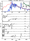Figure 5: Top panel: synthetic fit (blue) to observations (black) of SN1999em taken on the 14th of November 1999 (Leonard et al. 2002a). We also show the continuum flux level (red) computed by ignoring all bound-bound transitions in the formal solution of the radiative transfer equation. The model parameters are: $L_{\ast} = 1.5 \times 10^8~L_{\odot}$ , $R_{\rm phot} = 6.15 \times 10^{14}$ cm (or 8840 $R_{\odot }$ ), $v_{\rm phot}=6350$ km s^-1, $T_{\rm eff} =6800$ K, n=10, $\rho _{\rm phot} = 8.7 \times 10^{-14}$ g cm^-3. In the top panel, we insert a zoom on the Na I5596-5590 Å region: the green curve corresponds to the same model as above (blue) but with the sodium abundance enhanced to four times cosmic. Lower panel: montage of rectified spectra computed by including bound-bound transitions of individual species, limited to those that affect the emergent spectrum [color].

Open with DEXTER

Only optical data is available for SN1999em at this date so we rely entirely on the optical range to assess the UV flux level. The absence of He I lines and the increasing strength of Fe II lines are consistent with a much cooler effective temperature compared to the previously discussed models, associated with a strong line-blanketing in the UV range. The lower panel shows that this line-blocking stems mostly from Fe II, and to a lesser extent from Ni II, Ti II and Mg II (the 2800 Å feature). We find that as long as a big model atom for Fe II is included in our computations, the gross properties of the outflow and the emergent spectrum remain unchanged when adding extra metal species, e.g. Ni II.

The optical range clearly shows the presence of P-Cygni profiles from Ca II 3933-3968 Å and Ca II 8498-8542-8662 Å, which gives further support for a relatively low ionization of the outflow. Blends of H $\gamma$ , Ti II and Fe II contribute to the feature at 4300 Å while blends of Ti II, Mg II and Fe II contribute to the feature at 4600 Å. Around 5000 Å we see a myriad of Fe II lines which overlap with H $\beta$ , while Fe III lines are no longer predicted. The flux goes below the continuum level around 5500 Å, which we interpret as the appearance of the doublet line Na I 5896-5890 Å. Indeed, taking the same model and enhancing the sodium abundance by a factor of four (Fig. 5, top-panel, green curve in the inserted box), as expected for a supergiant progenitor (Prantzos et al. 1986), gives a much better fit to the observed sodium doublet. The dip on the blue-side of this sodium doublet has been associated with a number of Sc II lines (Leonard et al. 2002a), a species not yet included in our atomic database. Further to the red we reach a spectral region affected by weak Fe II lines which, in combination with Si II6347-6371 Å gives rise to some filling-in of the P-Cygni trough of H $\alpha$ .

As before, we show the outflow ionization predicted by the model (Fig. 6 - note that the highest ionization state of iron shown is Fe³⁺ but the lowest one is now Fe⁰⁺). Unlike the previous two cases hydrogen recombines to its neutral state, while in the corresponding region, iron is present in its Fe⁺ state (giving rise to the Fe II lines). Note that in the regions where hydrogen recombination takes place, the electron-density goes down more steeply with radius (this is seen by inspection of the spacing between tick marks on the top axis). The photosphere is located at r=1.48R₀ ( $\log(r/R_0) = 0.17$ ), right in the recombination front: hydrogen (iron) is equally represented in H⁺ and H⁰⁺ forms (Fe²⁺ and Fe⁺) while helium is fully neutral.

$\begin{figure} \par\epsfig{file=2525f6.eps, angle=-90, width=8cm,clip}\end{figure}$	Figure 6: Relative ionization for hydrogen (solid), helium (dashed) and iron (dash-dotted) for the late-stage model of Sect. 3.3. Note that the highest ionization state of iron shown is Fe³⁺ rather than Fe⁴⁺, but the lowest one is now Fe⁰⁺ rather than Fe⁺[color].
Open with DEXTER

4 Discussion on model results and properties

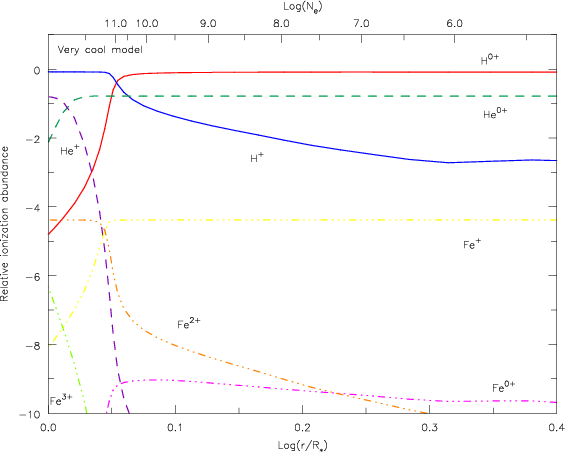
4.1 Hydrogen-recombination front in cool models

For models having an ionization similar or lower to the case shown in Sect. 3.3 (late-stage model), we had to introduce an adaptive grid in CMFGEN in order to resolve the region where hydrogen recombines. Indeed, this tends to occur over very restricted spatial scales in the outflow.

We show in Fig. 7 a plot of the outflow ionization for a very cool model with $T_{\rm eff} = 6000$ K. Note how steep the recombination of hydrogen is as well as the concomitant recombination of iron from Fe²⁺ to Fe⁺. Also shown is the radial variation of the electron-density (top axis); tick marks are more closely packed around the front, following the strong variation of the mean-electron number through this region.

$\begin{figure} \par\epsfig{file=2525f7.eps, angle=-90, width=8cm,clip}\end{figure}$	Figure 7: Relative ionization for hydrogen (solid), helium (dashed) and iron (dash-dotted) for a very cool model. For clarity, we only show the inner region of the outflow. The radial variation of the electron-density is also shown on the top axis [color].
Open with DEXTER

We find that the shape of the front depends on the spatial scale of the outflow, i.e. the bigger R₀ the more gradual the front is. Further, for identical model parameters, a smaller turbulent velocity gives reduced line-blanketing and thus a more extended hydrogen recombination front. Reducing the hydrogen abundance also reduces somewhat the steepness of the front. This may result from the fact that the electron-scattering optical depth is less tied to the front itself, which sets the position of the photosphere for H-rich models. Finally, varying the density exponent (see below) also modifies the shape of the recombination front, by extending it over larger spatial scales for smaller values of n.

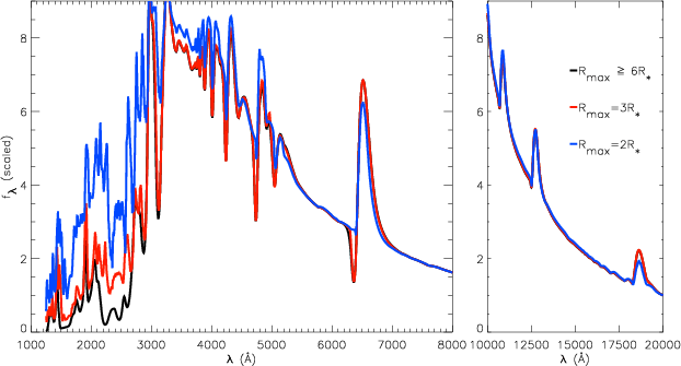
4.2 Choice of outer boundary

There is a strong computational incentive to limit the extent of the simulated grid. Ideally, the outer grid location should be where the medium becomes optically thin at all wavelengths. Unfortunately, H I and He I bound-free edges in the UV, as well as a few resonance lines remain optically thick even far above the photosphere. This occurs even though the density at r is only $(R_0/R_{\rm max})^n$ its value at R₀, n being of the order of 10. The drawback of stretching the computation to large radii is that the maximum velocity in the outflow can become very large, i.e. up to one third of the speed of light for the modeling, e.g., of the spectrum of SN1987A on the 24th of February 1987. In expanding outflows, a line with frequency $\nu_0$ at a given wind location rcan in principle interact with photons emitted at r' with a frequency between $\nu_0$ and $\nu_0 (1 + \vec{n} \cdot (\vec{v(r)} - \vec{v(r)'}))$ where $\vec{n}$ is the unit vector linking the two points of interest. The frequency sampling around line center must therefore be fine enough to account for potential line-transfer effects. But the larger the maximum velocity in the computation is, the larger is the frequency array and thus the more computationally demanding the model is.

In general, our simulations extend out to 10R₀. But we have investigated whether the choice of a bigger or a smaller maximum radius would produce a noticeable effect on the SED. Models suitable for the earlier evolution of type II SN during the photospheric phase (first week) tend to require a higher density exponent than at later times (see, e.g., Höflich 1988 for SN1987A; Eastman & Kirshner 1989), minimising the effect resulting from the modulation of the location of the maximum radius. For this check, we therefore have chosen a model with a density exponent of 8. This study is done with a small model atom, including only the most abundant species H I, He I, C II, N I, O I, Fe II, and Fe III.

$\begin{figure} \par\epsfig{file=2525f8.eps, width=8.8cm,clip}\end{figure}$

Figure 8: Comparison between emergent spectra computed with identical parameters but differing in the adopted maximum radius, chosen at 2 (blue), 3 (red) and 6, 10 and 15R₀ (overlapping perfectly to form the black curve). To facilitate the comparison of the relative synthetic fluxes for the different models, these have all been normalised to unity, at 10 000 Å ( left panel) and 20 000 Å ( right panel). R₀ is identical in all cases. Note also that the red and black curve overlap perfectly everywhere except in the UV. We employ a small model atom for this investigation, i.e. solely H I, He I, C II, N I, O I, Fe II, Fe III [color].

Open with DEXTER

We show in Fig. 8 the SED for models with a maximum radius of 2, 3, 6, 10, and 15R₀. For this latter case, we have modified the Hubble law by forcing it to smoothly plateau beyond 10R₀ to reach at 15R₀ only 110% of the value it has at 10R₀. Only three curves are seen in Fig. 8. Indeed, we find that the SED for the cases where $R_{\rm max} \ge 6 R_0$ are indistinguishable (they overlap under the black curve), a very desirable property which therefore justifies a significant reduction of the maximum radius. Out of curiosity, we have also reduced the maximum radius down to 3 (red curve) and finally 2R₀ (blue curve). Interestingly, beyond 3000 Å, the spectrum computed with $R_{\rm max} = 3 R_0$ , is indistinguishable from that computed with $R_{\rm max} = 6 R_0$ . This suggests that the continuum and line formation beyond 3000 Å is confined to the photosphere, located in these models at 1.8R₀. However, the UV flux lies significantly above the curve corresponding to the model with $R_{\rm max} = 6 R_0$ , which results from the neglect of line-blocking from the outflow layers between 3 and 6R₀. Indeed, metal lines in the UV remain optically thick far above the photosphere. Going down to $R_{\rm max} = 2 R_0$ , we see that the UV flux is even more in excess, for the same reason given as above, only magnified by the further reduction in maximum radius. But additionally, hydrogen lines (most notably H $\alpha$ , H $\beta$ , H $\gamma$ , P $\alpha$ ) are affected, both in emission and absorption. Note that the latter is nearly absent in H $\alpha$ , suggesting its P-Cygni trough forms over an extended region. In fact, adopting such a small value for $R_{\rm max}$ has a strong influence on the non-LTE solution of the problem. For example, we now find that the outer radius is optically thick throughout the wavelength range, so that there is no photosphere in this model!

Although the tests with $R_{\rm max}$ of 2 and 3R₀ presented only pedagogical material, the adequacy of choosing $R_{\rm max} = 6 R_0$ in our simulations is a very useful result.

4.3 Influence of metallicity on the emergent spectrum

As was shown in Sect. 3, line-blanketing becomes very effective in blocking the continuum star light as soon as the medium has cooled down sufficiently for Fe II to be present. The effective temperature at which this transition occurs is around 8000 K. Starting from the intermediate-stage model of Sect. 3.2, we have investigated what the impact would be of reducing or enhancing the metallicity, i.e. scaling all metal abundances by a factor of a half or two. 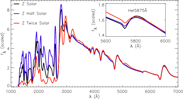We show the results in Fig. 9, where we reproduce the model of Sect. 3.2 in black, the twice-solar (half-solar) metallicity model in red (blue).

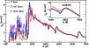$\begin{figure} \par\epsfig{file=2525f9.eps, width=8.8cm,clip}\end{figure}$

Figure 9: Comparison of the emergent flux from models with identical parameters apart from a different adopted metallicity. The black curve describes a model with solar metal abundance. The red (blue) shows the resulting emergent spectra when all metal abundances are scaled by a factor of two (one half). The model spectra beyond H $\alpha$ are relatively insensitive to changes in metallicity - therefore for ease of comparison we have normalised the fluxes to unity at 7000 Å [color].

Open with DEXTER

It thus seems that the UV SED can be used to constrain the environmental metallicity at early times when the line-blocking due to the Fe II lines is still moderate. At later times, e.g., for the late-stage model discussed in Sect. 3.3, the UV flux is negligible and thus placing constraints on the metallicity has to be done from the optical - there are no strong iron lines at longer wavelengths. Strong line-overlap makes this task difficult. Finally, note that the probability of seeing metals nucleosynthesized during the explosion increases with time so the primordial metallicity of the progenitor can be more reliably constrained from spectra taken at earlier times.

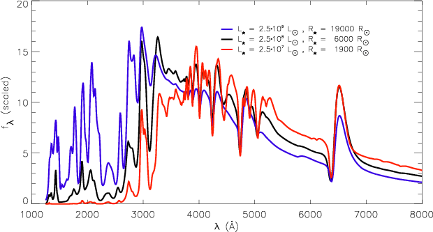
4.4 Influence of luminosity

When modeling SN there is always an uncertainty in its distance. In this section we therefore investigate how the synthetic flux distribution changes with luminosity. Note that in our current approach the luminosity of the model is adjusted so that, for an adopted Cepheid distance, the model flux distribution lies within a factor of 2 of that observed. In the future, it will be desirable to modify CMFGEN in order to use a SN luminosity computed from a hydrodynamical simulation of the explosion.

We show in Fig. 10 a set of three models differing in model luminosity (black curve: $L_{\ast} = 2.5 \times 10^8~L_{\odot}$ ; blue curve: $L_{\ast} = 2.5 \times 10^9~L_{\odot}$ ; red curve: $L_{\ast} = 2.5 \times 10^7~L_{\odot}$ ). In order to maintain a similar total base continuum optical depth and effective temperature, we scale up (down) the base radius by $\sqrt {10}$ and scale down (up) the base density for the model corresponding to the blue (red) curve. To position the three models in the same figure, we display the flux of the blue (red) model scaled down (up) by a factor of 10. With this scaling the model that has a higher flux in the UV has a lower flux in the optical and vice-versa, a likely result of the modulation of line-blanketing due to the variation in spatial scale of the corresponding model. Note that we use a small model atom, including only the most abundant species H I, He I, C II, N I, O I, Fe II and Fe III.

$\begin{figure} \par\epsfig{file=2525f10.eps, width=8.8cm,clip}\end{figure}$

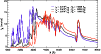Figure 10: Comparison of the emergent flux from models differing in luminosity, enhanced and decreased by a factor of ten compared to the model in black. Also, we scale the radius and the base density up or down by $\sqrt {10}$ , to maintain the same photospheric velocity for all (see text for details). The model atom used is small, including only the most abundant species, i.e. H I, He I, C II, N I, O I, Fe II and Fe III [color].

Open with DEXTER

These various model scalings lead to a very similar photospheric velocity, i.e. 6700 km s^-1 (red curve) and 7200 km s^-1 for both black and blue curves, as can be seen from the nearly overlapping positions of absorption in line features. As expected from Fig. 10, the effective model temperature increases from the red ( $T_{\rm eff} = 7000$ K), to the black ( $T_{\rm eff} = 7900$ K) and blue model ( $T_{\rm eff} = 8400$ K). The reason for this is that the photospheric density varies a great deal amongst those three models, increasing from high to low luminosity models (blue: $\rho_{\rm phot} = 0.88 \times 10^{14}$ g cm^-3; black: $\rho_{\rm phot} = 2.8 \times 10^{14}$ g cm^-3; red: $\rho_{\rm phot} = 16.3 \times 10^{14}$ g cm^-3). The higher the photospheric density the stronger the line-blanketing and the more depleted the UV flux appears.

Thus, when a large flux difference between a model and a given observation exists, a satisfactory fit to the observed energy distribution will likely become poor once the model and observed flux levels are comparable. We find that little or no changes are observable in the synthetic flux distribution when the luminosity is varied by a factor of two, so this sets the error one can make on the model luminosity when performing fits to observations.

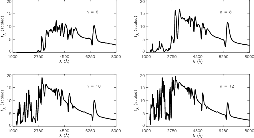
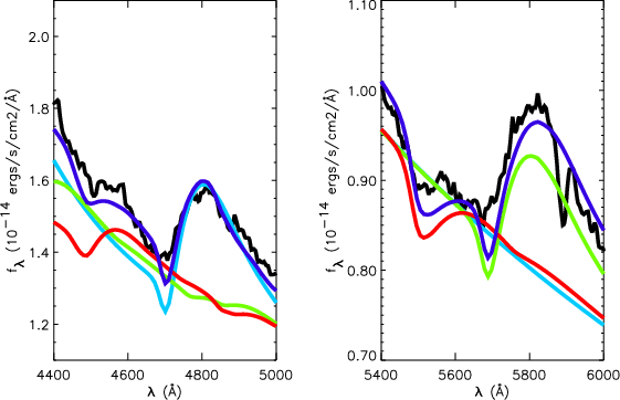
4.5 Effects of varying the density exponent

In our approach, we use an analytical description of the outflow density, characterized by a base density $\rho_{0,n}$ and a density exponent n so that at a given height r, we have $\rho(r) = \rho_{0,n} (R_{\ast}/r)^n$ . To ensure that the diffusion approximation is fulfilled at the base of the envelope, the base density is chosen so that the total continuum optical depth of the outflow is approximately 50. The density exponent is, however, constrained from observations. We have therefore a lot more flexibility than if we based our calculations on hydrodynamical inputs, for which the density distribution is set once and for all at the start of the homologous expansion. This flexibility is not necessarily a benefit since varying the density exponent can influence the emergent spectrum in a variety of ways, widening considerably the already large parameter space.

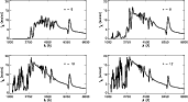$\begin{figure} \par\epsfig{file=2525f11.eps, width=15cm,clip}\end{figure}$	Figure 11: Illustration of the influence of the density exponent n on the synthetic flux distribution for n=6, 8, 10 and 12. All other model parameters are kept identical. The model atom used is small, including only the most abundant species, i.e. H I, He I, C II, N I, O I, Fe II and Fe III.
Open with DEXTER

In the previous section, we saw that the spatial scale of the expanding SN can affect significantly the emergent spectrum, mostly from the variation of the photospheric density. Let us assume that the model is fully ionized and that the continuum opacity is mostly due to electron-scattering ( $\kappa_{\rm e} \sim 0.34$ cm²/g), and investigate how model properties are affected by a change in the characteristics of the density distribution. Along a radial ray, the continuum optical-depth is given by $\tau(r) = \int_r^{\infty} \kappa_{\rm e} \rho(r') {\rm d}r'$ so that at the photosphere, we have $\tau_{\rm phot} = \frac{\kappa_{\rm e} \rho_{0,n} R_{\ast}}{n-1} \left( \frac{R_{\ast}}{R_{{\rm phot},n}} \right)^{n-1}$ .

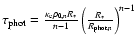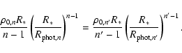
Let us take another model identical in all parameters except for those that characterize the density distribution (n', $\rho_{0,n'}$ , $R_{{\rm phot},n'}$ ) and compare these at the photosphere:

We show in Fig. 11 the synthetic spectra of models differing solely in density exponent n - in particular the base density is kept constant - covering values of 6, 8, 10 and 12. We clearly see that as the exponent is increased, the spectrum shows a more and more pronounced UV flux, metal lines of decreasing strength in the optical but a strengthening He I 5875 Å. As expected, the photospheric radius decreases from 1.9, to 1.81, 1.54 and 1.4 times the base radius (kept constant) as one goes from n=6 to 12. Given the adopted Hubble law, a similar decrease in photospheric velocity follows (from 7600 to 7250, 6150 and 5600 km s^-1). But there is a significant rise of the effective temperature over that range, from 6400, to 7900, 8100 and 8250 K. These effects are reversed if instead one maintains the photospheric radius rather than the base density when changing the density exponent (Eastman & Kirshner 1989).

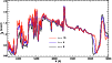$\begin{figure} \par\epsfig{file=2525f12.eps, width=8.8cm,clip}\end{figure}$	Figure 12: Illustration of the influence of the density exponent n on the synthetic flux distribution for n=6, 8, 10 in a cool model where hydrogen recombines near the base. All other model parameters are kept identical. Note that the most striking effect is on the set of Ca II lines near 8500 Å, the line appearing broader and stronger for smaller density exponents [color].
Open with DEXTER

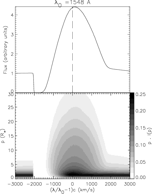
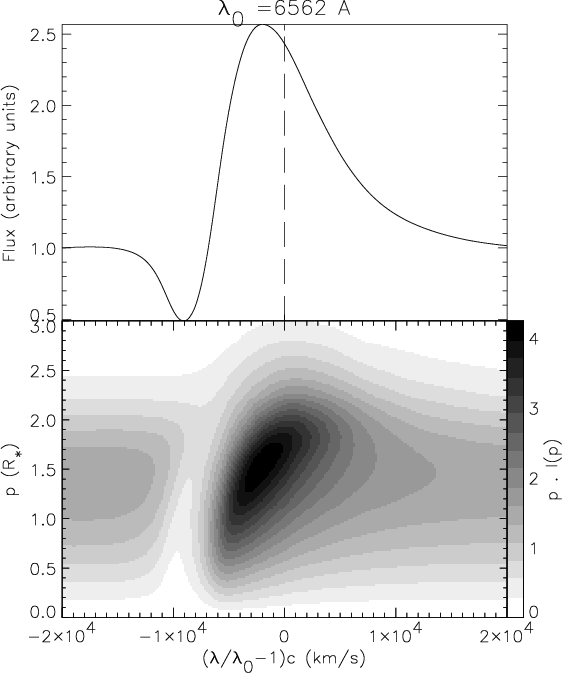
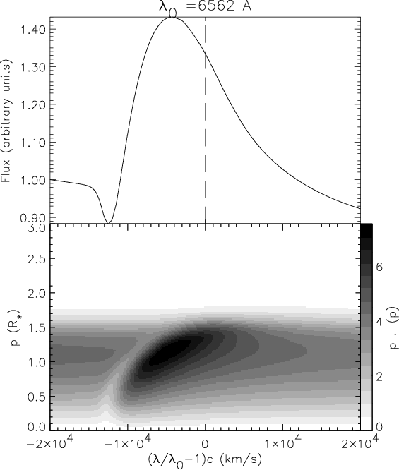
Besides the general influence on the spectral energy distribution, changing the density exponent has also a significant effect on line profiles. For example, there is a systematic blue-shift of the observed H $\alpha$ P-Cygni profile in type II SN, which can be modulated in models by changing the density exponent (Sect. 5). Here we illustrate the influence the density exponent has on the strength and width of the Ca II feature near 8500 Å. This set of lines is present only in models that are cool enough, i.e. those where hydrogen recombines at the photosphere. 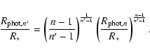We show in Fig. 12 the synthetic flux distribution of three models differing only in density exponent (n=6, 8 and 10). Contrary to the previous figure, the effect on the overall spectrum is small, mostly because in this parameter space, the line and continuum formation is essentially contained within the (localized) region of the recombination front. 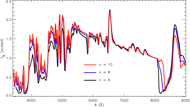However, as shown in Fig. 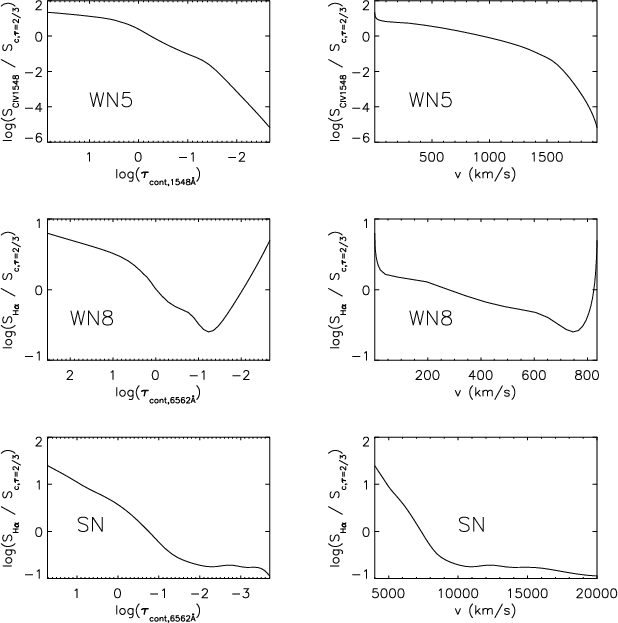13, the Ca II lines at 8498, 8542 and 8662 Å form over the entire outflow and are therefore extremely sensitive to the density gradient even above the recombination front, resulting in a broader and stronger Ca II feature for smaller exponents. However, H $\alpha$ is more confined to the photosphere region and is thus only weakly sensitive to the outer density distribution. This explains why this set of Ca II lines can be used to reveal the presence of outflow asymmetry, as inferred, e.g., by Kasen et al. (2003) in the type Ia SN2001el, from the presence of strong polarization (with a different angle) in this Ca II spectral region compared to the rest of the spectrum. This line can therefore be used as a diagnostic for the density distribution and/or departure from sphericity of SN outflows in general, when ionization conditions in the outflow are suitable, i.e. for effective temperatures at and below 8000 K.

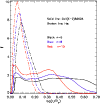$\begin{figure} \par\epsfig{file=2525f13.eps, width=8.8cm,clip}\end{figure}$

Figure 13: Illustration of the relative line emission occurring at a given height in the outflow, both for one of the three components of the Ca II feature at ca. 8500 Å, i.e. Ca II8662 Å (solid line) and H $\alpha$ (broken line). We use a color coding to differentiate between models with different density exponent. Note how extended the line formation region of the Ca II line is compared to that of H $\alpha$ . The other two components of the Ca II triplet show a similar behavior and are thus not shown. $\xi$ is defined such that line flux is proportional to $\int \xi {\rm d}\log r$ [color].

Open with DEXTER

4.6 Lines of selected species

4.6.1 Hydrogen lines

At present there is an open debate concerning the capability of model atmospheres to fit the hydrogen Balmer lines of type II SN during the photospheric phase. Some groups fail to reproduce these lines (Schmutz et al. 1990; Mitchell et al. 2002, both for SN1987A) while others fit them very well (Eastman & Kirshner 1989; Höflich 1988, again for SN1987A). Schmutz et al. invoked the possibility of clumping although they did not investigate whether it could in reality cure the problem, while a decade later, Mitchell et al. invoked energy deposition following ⁵⁶Ni mixing in the outer envelope of SN1987A, as soon as 4 days after core-collapse. Those who fit the hydrogen Balmer lines well for the same dates do not use clumping and ignore energy deposition.

This situation is unsatisfactory since it is difficult to establish whether the problem is physical or numerical. We have shown in the previous section that CMFGEN reproduces extremely well the hydrogen Balmer lines, even though we overplot the synthetic spectrum and adopt a linear flux scale, two elements that have the potential to make fit discrepancies very clear. Although we show in Sect. 3 only three cases, all synthetic spectra computed for SN1987A and SN1999em fit the observations very well, provided that a strong hydrogen recombination front does not develop, i.e. as long as hydrogen remains mostly ionized in the outflow. Indeed, if such a front appeared, CMFGEN always predicted H $\alpha$ too weak by a factor of 2-3 compared to observations, both for the emission and absorption components (see for example the H $\alpha$ region in the cool models shown in Fig. 12).

In CMFGEN, whose principal purpose is to determine the atmospheric structure and level populations, we simply adopt a Gaussian shape, of constant width, to describe the intrinsic profile. In practice, the width of the profiles is set by the adopted micro-turbulent velocity. To save computational time, we have chosen a turbulent velocity $v_{\rm turb}$ of 100 km s^-1. For fully ionized models, varying this value by a factor 2-3 has no effect on the emergent spectrum. However, for cooler models, we find that reducing this turbulence to 20 km s^-1is important in order to reproduce better the profile shape and strength of H $\alpha$ . In those cool models, a lower turbulent velocity gives a SED with a higher flux in the UV, and essentially a higher apparent outflow ionization (in fully ionized models, the effect on the SED is unnoticeable). We understand this as resulting from the reduced line-blanketing, itself stemming from the reduced spectral band-width over which metal lines block the ionizing flux emanating from the thermalisation layer at the base. Similarly, late-stage simulations performed with fewer metal species show an appreciable increase in the H $\alpha$ strength, again likely to result from the modulated amount of line-blanketing.

4.6.2 Helium lines

We show in Fig. 14 CMFGEN fits to He I 5875 Å observed in SN1999em on the 30th of October and on the 1st, 5th and 8th of November 1999 (Leonard et al. 2002a). The quality of the fits is very good, with only a modest helium enrichment ( ${\rm H/He}=5$ by number).

$\begin{figure} \par\epsfig{file=2525f14.eps, width=8cm,clip}\end{figure}$

Figure 14: Synthetic fits (broken line) to observations (solid line) of SN1999em taken on the 30th of October (A), and the 1st (B), 5th (C) and 8th (D) of November 1999 (Leonard et al. 2002a), showing the He I 5875 Å line region. Note how well CMFGEN manages to reproduce the observed profile using only a modest helium enrichment over the cosmic value ( ${\rm H/He}=5$ by number), in agreement with stellar evolutionary predictions for Blue/Red supergiants, progenitors of type II SN. This capability of CMFGEN is in stark contrast with failures to reproduce this He I line in the works of Schmutz et al. (1990) and Eastman & Kirshner (1989), suggesting the importance of treating all species in non-LTE.

Open with DEXTER

4.6.3 Nitrogen lines

Based on a direct analysis with SYNOW, Baron et al. (2000) proposed that the feature blue-ward of He I 5875 Å in the spectrum of SN1999em taken on the 30th of October was due to N II. However, they could not confirm this statement with the more detailed analysis done with PHOENIX. They also highlighted the presence of a kink in the blue wing of H $\beta$ , which they do not associate with N II, but rather to some peculiar emission process occurring in the outflow. Similar intriguing features were observed in the early spectra of another type II SN, SN1999gi by Leonard et al. (2002b). They observed the presence of un-identified features in the blue wing of both He I 5875 Å and H $\beta$ , at blue-shifted velocities of ca. 20 000 to 30 000 km s^-1 although, these have now clearly-defined P-Cygni profile shapes. Given the relatively higher density exponent characterizing the outflows of type II SN at earlier dates, it seems unlikely that much emission could arise at velocities (or distances), a few times the value at the photosphere, especially in recombination lines since these have a density-square dependent emissivity.

$\begin{figure} \par\epsfig{file=2525f15.eps, width=8cm,clip}\end{figure}$

Figure 15: Zoom into the optical spectroscopic observations (black) of SN1999em taken on the 30th of October 1999 (Leonard et al. 2002a) showing synthetic fits for a model comprising all species as given in Table 1 (blue) or only bound-bound transitions of hydrogen (turquoise), helium (green) and nitrogen (red). We strongly support the idea that the observed features around 4600 Å and 5500 Å are due to N II lines [color].

Open with DEXTER

We show in Fig. 15 synthetic fits to observations of SN1999em taken on the 30th of October 1999 (Leonard et al. 2002a). The dark-blue curve corresponds to the emergent spectrum when all species are included. It fits well the He I 5875 Åand H $\beta$ regions, although a slightly higher expansion velocity would improve the fit to the He I line (i.e., a shift of the line formation region to larger velocities). Note the presence of kinks at around 4600 Å and 5500 Å, i.e. in the blueward region of each of these two lines. We over-plot the emergent spectra with bound-bound transitions exclusively of hydrogen (turquoise), helium (green) and nitrogen (red curve), normalizing all curves to the observed flux at 8000 Å. Unlike PHOENIX, CMFGEN is capable of reproducing the N II line in the blue wing of He I 5875 Å, but together with this line, it also predicts the equally strong N II feature around 4600 Å. In our model, these correspond to multiplets of N II(3d-3p) centered around 4480 Å and 5490 Å, as well as N II(3p-3s) at 4630 Å and 5680 Å.

The reason for the different results between PHOENIX and CMFGEN, regarding the N II lines and the kink in the blue wing of H $\beta$ , is unclear. Our fits to hydrogen Balmer line profiles are much better, in particular the width and depth of the troughs, giving us confidence that we are not predicting spurious absorption too far to the blue of line-centers. Moreover, their Fig. 6 suggests that not just H $\beta$ shows a kink beyond the point where the absorption trough meets the continuum, but that this feature is also present at a similar location for He I5875 Å and H $\alpha$ (note that their use of a very thick line makes this difficult to see). Such a kink is however not observed in H $\alpha$ (see their Fig. 3).

Our model fits show unambiguously that nitrogen lines are present in the optical spectrum of the early photospheric phase of SN1999em. In SN1999gi, spectroscopic observations taken after the 12th of December 1999 are very similar to those of SN1999em, so that we reach the same conclusion. Note however that for the first spectrum of SN1999gi (taken on the 10th of December 1999), the feature at ca. 4600 Å is much stronger than that at ca. 5500 Å, a situation we have not been able to reproduce. By the 12th, the feature has both receded and weakened and is then well reproduced (and identified as an N II line) by our model for SN1999em on the 30th of October 1999 (Fig. 15). In our model, we use a factor ten enrichment of nitrogen compared to cosmic while we find that these N II features become unnoticeable when this factor becomes smaller than around 3. This strongly supports the idea that the progenitors of SN1999em and SN1999gi had core-processed nitrogen at their surface at the time of collapse.

Interestingly, although the first spectrum of SN1987A shows the high ionization conditions for the presence of these N II features, these are not observed. Together with the fact that a modest helium enhancement permits a nice fit of the spectrum, this suggests that the pre-collapse progenitor of SN1987A had a surface abundance closer to the current LMC abundances. Hence, identification of N II lines is a significant clue for enhanced nitrogen abundance in the outer layers of the progenitor star. Note that the over-abundance of nitrogen should be accompanied by a significant depletion of carbon and oxygen if it resulted mostly from the peeling-off of the outer envelope through a stellar wind mass loss. In the case of mixing, which can for example be made more efficient through stellar rotation, a more modest depletion in carbon and oxygen would result. Unfortunately, we have not been able to identify lines from either of these species in the photospheric phase of type II SN, although the addition of C I in our model atom could alter this conclusion. We defer until a future study a proper discussion on this issue.

5 Line formation in expanding outflows of hot stars and type II SN

Before concluding on these premiminary results with CMFGEN, we present a study on the formation of P-Cygni line profiles in type II SN outflows, which reveals subtle differences from that observed, e.g., in the eponymous star. Indeed, a striking feature in early-time spectra of type II SN is the large blue-shift, by as much as ca. 100-150 Å (5000-7000 km s^-1), of the H $\alpha$ line profile compared to the rest wavelength of 6562.79 Å. At later times, this blue-shift is less obvious, partially because the photospheric velocity quickly decreases, but it is nonetheless present (see, e.g., Pastorello 2004).

To investigate the origin of this feature, we first focus on the formation of scattering (resonance) and recombination lines in Wolf-Rayet outflows. Their density distribution is much flatter than that of SN, following roughly a 1/r² law (imposed by mass conservation); non-LTE effects are important but line-formation occurs over much larger spatial scales compared to the photospheric radius. Therefore, these objects offer a nice counterpart to line-formation conditions in SN, which we are trying to understand.

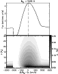$\begin{figure} \par\epsfig{file=2525f16.eps, width=7.4cm,clip}\end{figure}$

Figure 16: Hot star model (WN5). Bottom: grayscale image of the quantity $p \cdot I(p)$ as a function of pand scaled wavelength $x=(\lambda /\lambda _0-1)c$ , where p is the impact parameter (in units of the hydrostatic radius $R_{\ast }$ ), I(p) the specific intensity along p (at x). Here, $\lambda _0$ corresponds to the rest wavelength of C IV 1548 Å and cis the speed of light. The terminal velocity of the model is 2000 km s^-1. Top: line profile flux, directly obtained by summing $p \cdot I(p)$ over the range of p. Thus, the line flux at x in the top panel corresponds to the cumulative sum of all contributions $p \cdot I(p)$ at x shown in the bottom panel, giving a vivid illustration of the sites at the origin of the observed line profile.

Open with DEXTER

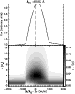$\begin{figure} \par\epsfig{file=2525f17.eps, width=7.4cm,clip}\end{figure}$	Figure 17: Hot star case (WN8) Same set as in Fig. 16 but for the H $\alpha$ line in a WN8 model with a terminal velocity of 840 km s^-1.
Open with DEXTER

We are particularly interested in determining where in the outflow the emergent flux originates from. Using models for nitrogen-rich Wolf-Rayet (WN) stars similar to those studied elsewhere (e.g., Hillier & Millier 1998; Herald et al. 2001), we show in Figs. 16-17 gray-scale images in the (x,p) plane of the flux-like quantity $p \cdot I(p)$ , where $x = (\lambda/\lambda_0-1)~c$ , $\lambda$ is the wavelength, p is the impact parameter and I(p) is the specific intensity (at $\lambda$ , or x). Note here that p is in units of the hydrostatic radius $R_{\ast }$ of the WN star under consideration. In Fig. 16 (WN5 case), we show the case of the resonance line C IV 1548 Å in a hot hydrogen-free WN model with an asymptotic velocity $v_{\infty} = 2000$ km s^-1, while in Fig. 17 (WN8 case), we show the case of the recombination line H $\alpha$ in a cooler (hydrogen-rich) WN model (with $v_{\infty} = 840$ km s^-1). In each figure, the top panel shows the synthetic line profile, which, for any scaled velocity x, corresponds to the integral over all p of the quantity $p \cdot I(p)$ plotted in the lower panel. Thus, for any x, we directly identify the contribution at p of the relative fraction made to the total line profile flux.

The gray-scale illustrations contain a lot of information. First, beyond the velocity limits of the line (limited naturally to $\pm v_{\infty}$ ), we primarily observe continuum photons, although some line photons are observed outside this range (primarily on the red side) due to the effects of incoherent electron scattering. In Fig. 16, the continuum photons originate at p values up to about $p_{\rm lim} = 5 R_{\ast}$ , which is the location of the photosphere in this WN star model. In Fig. 17, we observe a similar effect, although the photosphere is much closer in, at ca. $2 R_{\ast}$ . But in both cases, the line remains optically-thick out to much larger values of p - a few tens of the corresponding $R_{\ast }$ . This is consistent with the generally-accepted fact that line formation in Wolf-Rayet outflows occurs over large scales compared to the photospheric radius.

Although the lower panels of Figs. 16 and 17 look qualitatively similar, Fig. 16 shows a P-Cygni profile, while Fig. 17 shows an emission profile. Close inspection of the lower panels shows that emission beyond $p_{\rm lim}$ is strong, roughly symmetric about line center (modulo turbulence effects): a key difference is that emission extends up to $v_{\rm frac} \sim 0.5 v_{\infty}$ for the WN5 model (Fig. 16) but right up to $v_{\rm frac} \sim v_{\infty}$ for the WN8 model (Fig. 17). In both cases there is a strong flux deficit on the blue side for $p < p_{\rm lim}$ , which is compensated for in the line profile, but only up to $\pm$ $v_{\rm frac}$ , by the line flux emitted at larger impact parameters. For the WN5 case, absorption beyond -1000 km s^-1 is not compensated by emission and a trough appears in the resulting profile. For the WN8 case, absorption merely introduces skewness in an otherwise pure emission profile.

Let us now consider the case of a type II SN, taking a model similar to that presented in Sect. 3.2. We show the equivalent of Figs. 16 and 17 for that SN case in Fig. 18 for H $\alpha$ . $R_{\ast }$ now refers to the base radius of the simulation also called R₀. The difference with the Wolf-Rayet case is large. Line and continua are confined to similar regions, both becoming optically-thin beyond $p_{\rm lim}=2 R_{\ast}$ . Interestingly, both emission and absorption occur below $p_{\rm lim}$ . Emission thus only appears on the blue side of the profile, which explains why the resulting emission profile is strongly blue-shifted. This occurs because the density drop-off is high in type II SN (n=10 in this model) so that emission is favored in the inner denser regions, strengthening the impact of disk-occultation and continuum optical depth effects.

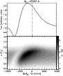$\begin{figure} \par\epsfig{file=2525f18.eps, width=8cm,clip}\end{figure}$	Figure 18: Type II SN model Same set as in Figs. 16 and 17 for the H $\alpha$ line formed in a SN outflow with similar properties to those described in Sect. 3.2.
Open with DEXTER

What controls the different behaviors shown in Figs. 16-18 is the radial variation of the line source function $S_{\rm l}$ compared to the continuum source function at a radial optical depth of approximately $\tau_{\rm c}=2/3$ . We show in Fig. 19 plots of $S_{\rm l}/S_{\rm c}(\tau_{\rm c}=2/3)$ versus continuum optical depth and versus radial velocity for the three models. Consider a photospheric (core) ray. The continuum intensity emanating from that ray is approximately $S_{\rm c}(\tau_{\rm c}=1)$ ( $\approx$ $S_{\rm c}(\tau_{\rm c}=2/3)$ ), where $\tau_{\rm c}$ now refers to the optical depth along the ray and we have made use of the Eddington-Barbier relation. On the other hand, the intensity in an optically thick line at some frequency in the line will simply be the line source function at the resonance zone for that frequency. For the WN5 star we see that the line source function is less than the reference continuum source function for $\tau_{\rm c} < 2/3$ and V > 900 km s^-1, and drops to very small values for V>1200 km s^-1. Thus we expect no emission (as compared to the continuum) for V > 1200 km s^-1, as indeed seen in Fig. 16. For the WN8 star the H $\alpha$ source function is less than $S_{\rm c}(\tau_{\rm c}=2/3)$ beyond 300 km s^-1, but it drops, by at most a factor of 4 at 750 km s^-1. Thus the flux is reduced relative to the continuum, but never goes black. The reduced flux is easily compensated by emission from rays not striking the photosphere, and hence we see no P-Cygni profile.

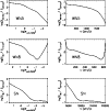$\begin{figure} \par\epsfig{file=2525f19.eps, width=8.8cm,clip}\end{figure}$	Figure 19: Radial and velocity variation of the logarithm of the line source function normalized to the continuum source function at a continuum optical depth of two third (see text for details). We show the cases corresponding to Figs. 16-18, i.e. for C IV 1548 in the WN5 model ( top), H $\alpha$ in the WN8 model ( middle) and H $\alpha$ in the SN model ( bottom).
Open with DEXTER

The SN model is different yet again. From Fig. 19, we see the line source function drops below the continuum source function for velocities greater than 7000 km s^-1. Thus, for such velocities, we expect to see reduced emission, as seen from Fig. 18. Further, because the continuum opacity is mainly due to electron scattering, we can see emission arising from optical depths greater than $\tau_{\rm c}=1$ (V < 7000 km s^-1). Because the line source function is larger than the continuum in this region, the line is in emission. This is again seen in Fig. 18. Unlike the two WR models, we get significant emission for rays striking the photosphere. Because (by definition) the photosphere is thick we do not see much emission from the backside of the flow. Consequently the emission, for photospheric rays, is strongly skewed to the blue (Fig. 18).

Finally, we show in Figs. 20 and 21 the cases for SN models that have different density exponents, i.e. n=8 and n=14 respectively compared to the model shown in Fig. 18. Indeed, the higher n is, the faster the density drops and the more blue-shifted the resulting H $\alpha$ profile looks. While the source function follows a similar trend in these two additional cases (not shown), it is the modulated influence of disk occultation and continuum optical depth effects that give rise to different blue-shift magnitudes in the resulting profile. Overall, the large density exponent characterizing the early evolution of type II SN is also a key ingredient that precludes the possibility of observing a clear departure from sphericity (if at all present), the line and continuum formation regions overlapping in space and being so confined.

6 Conclusion

We have presented first results based on the model atmosphere code CMFGEN (Hillier & Miller 1998) for the spectroscopic modeling of photospheric-phase type II supernovae. To facilitate the modeling, several changes were made to the code: these include the ability to use a Hubble velocity law and a power-law density distribution, an adaptive grid to handle the steep H recombination front in cooler SN models, and an improved algorithm to compute the gray temperature distribution in a rapidly expanding outflow. Still to be included in our treatment are relativistic effects, energy deposition from radioactive decay, and the possibility to base our computation on a computed hydrodynamical structure. We demonstrated the ability of CMFGEN to reproduce a large number of features in high S/N multi-wavelength spectroscopic observations of type II SN, using the very well-observed SN1987A and SN1999em. The observed spectral energy distribution from UV to the near-IR (when available) can be matched very accurately: the fit quality is in general within the 10% level, although it is difficult to match observations in the UV range to better than 20-30%. We show examples taken over a wide range of outflow ionization properties, covering fully- (early-time) and partially- (late-time) ionized spectra. This good behavior of CMFGEN gives us hope that a wealth of information can be retrieved through a detailed analysis of multi-epoch observations of type II SN. Based on a representative set of observations, we show that He I lines in early-time spectra can be well fitted by invoking modest helium enrichment typical of an OB-supergiant progenitor. The non-LTE radiative transfer solution also predicts the presence of lines in the optical from higher ionization than before expected, in particular Fe III and N II. The latter provides a simple explanation for the appearance of "bumps'' in the blue-wing of H $\beta$ and He I 5875 Å, generally interpreted in terms of over-dense emitting (in the corresponding line) structures lying far above the photosphere. Overall, this study shows that taking into account as accurately as possible the enormous effects of line-blanketing is key for a detailed modeling of type II SN. We also discuss through a number of different stand-points the problem of line and continuum formation in type II SN, giving vivid illustrations for both. In particular, for the first time, we give an illustration to explain the sometimes strong blue-ward wavelength shift of, e.g., H $\alpha$ in type II SN. The shift arises from the combined effects of disk-occultation, continuum optical depth effects, and a line formation region confined to the photosphere.

Forthcoming studies will present more focused analyses on specific issues. Since most investigations done on type II SN are with the aim of using them for the distance calibration of the Universe (as holds for Ia's), we will next study the Expanding Photosphere Method and the analysis of Eastman et al. (1996), following their approach but using CMFGEN to search for possible differences, in, e.g., correction factors. We will also discuss methods for determining the photospheric velocity, an issue of importance since the rate of expansion of the radiating photosphere is one of the key quantities entering any such distance determination. Long term goals are to design a very reliable method to determine distances in the Universe based on type II SN, with application to a sample of very well observed objects. Analyses of individual objects is also sought, in order to constrain the evolutionary status of the SN progenitor based on a spectroscopic approach, to complement inferences made exclusively from photometric measurements performed on the pre-explosion object (see, e.g., Smarrt et al. 2004).

Quantitative spectroscopy of photospheric-phase type II supernovae

1 Introduction

2 Presentation of the code

3 Spectroscopic modeling

3.1 Early stage

3.2 Intermediate stage

3.3 Late stage

4 Discussion on model results and properties

4.1 Hydrogen-recombination front in cool models

4.2 Choice of outer boundary

4.3 Influence of metallicity on the emergent spectrum

4.4 Influence of luminosity

4.5 Effects of varying the density exponent

4.6 Lines of selected species

4.6.1 Hydrogen lines

4.6.2 Helium lines

4.6.3 Nitrogen lines

5 Line formation in expanding outflows of hot stars and type II SN

6 Conclusion

References

$\begin{figure} \par\epsfig{file=2525f20.eps , width=8cm,clip}\end{figure}$	Figure 20: Same as Fig. 18 for a model with n=8.
Open with DEXTER

$\begin{figure} \par\epsfig{file=2525f21.eps, width=8cm,clip}\end{figure}$	Figure 21: Same as Fig.18 but for a model with n=14.
Open with DEXTER