 |
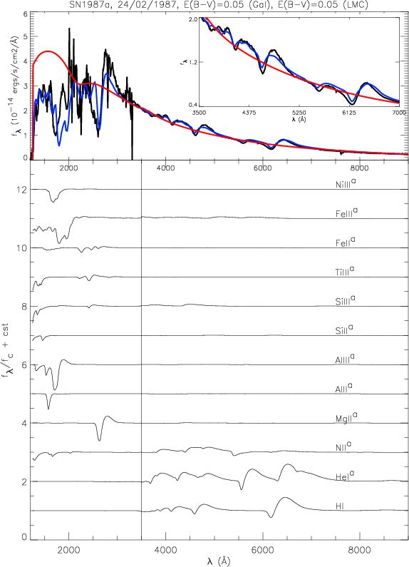
Figure 1:
Top: illustration showing the comparison between reddened model spectra (blue)
and observations of SN1987A (black) taken on the 24th of February 1987
(Pun et al. 1995; Phillips et al. 1988).
Each model flux distribution is scaled for an assumed LMC distance of 52 kpc.
In red we show the theoretical continuum energy distribution of the
model.
Model characteristics are:
|
| Open with DEXTER | |
In the text
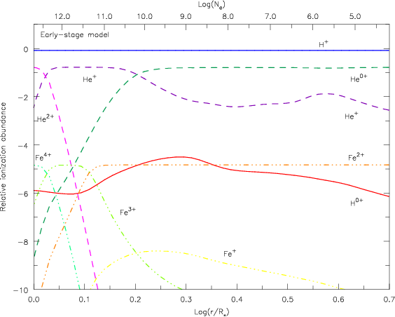 |
Figure 2: Relative ionization for hydrogen (solid), helium (dashed) and iron (dash-dotted line) for the early-stage model of Sect. 3.1 and Fig. 1. The ionization fractions are expressed relative to the abundance of all species. Also shown is the electron density on the top axis [color]. |
| Open with DEXTER | |
In the text
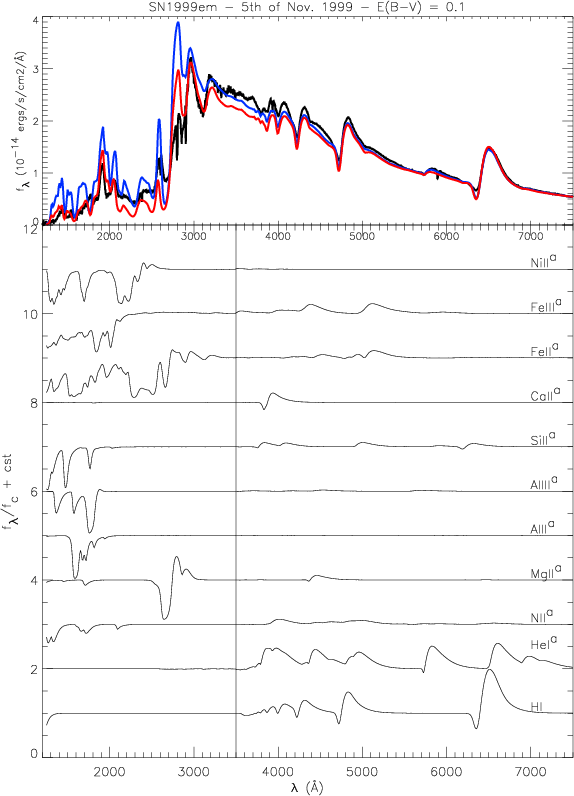 |
Figure 3:
Top panel: synthetic fit (color) to HST and Lick observations (black)
of SN1999em taken on the 5th of November 1999 (Baron et al. 2000; Leonard et al. 2002a). The red (blue) curve corresponds to a model with
|
| Open with DEXTER | |
In the text
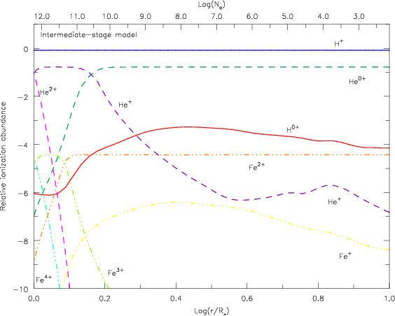 |
Figure 4: Ionization structure for the intermediate-stage model described in Sect. 3.2 and shown in Fig. 3. The ionization fractions are expressed relative to the abundance of all species [color]. |
| Open with DEXTER | |
In the text
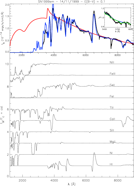 |
Figure 5:
Top panel: synthetic fit (blue) to observations (black) of SN1999em taken
on the 14th of November 1999 (Leonard et al. 2002a). We also show the continuum
flux level (red) computed by ignoring all bound-bound transitions in the formal
solution of the radiative transfer equation.
The model parameters are:
|
| Open with DEXTER | |
In the text
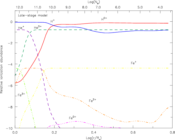 |
Figure 6: Relative ionization for hydrogen (solid), helium (dashed) and iron (dash-dotted) for the late-stage model of Sect. 3.3. Note that the highest ionization state of iron shown is Fe3+ rather than Fe4+, but the lowest one is now Fe0+ rather than Fe+[color]. |
| Open with DEXTER | |
In the text
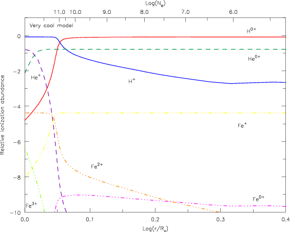 |
Figure 7: Relative ionization for hydrogen (solid), helium (dashed) and iron (dash-dotted) for a very cool model. For clarity, we only show the inner region of the outflow. The radial variation of the electron-density is also shown on the top axis [color]. |
| Open with DEXTER | |
In the text
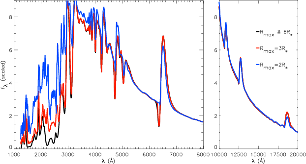 |
Figure 8: Comparison between emergent spectra computed with identical parameters but differing in the adopted maximum radius, chosen at 2 (blue), 3 (red) and 6, 10 and 15R0 (overlapping perfectly to form the black curve). To facilitate the comparison of the relative synthetic fluxes for the different models, these have all been normalised to unity, at 10 000 Å ( left panel) and 20 000 Å ( right panel). R0 is identical in all cases. Note also that the red and black curve overlap perfectly everywhere except in the UV. We employ a small model atom for this investigation, i.e. solely H I, He I, C II, N I, O I, Fe II, Fe III [color]. |
| Open with DEXTER | |
In the text
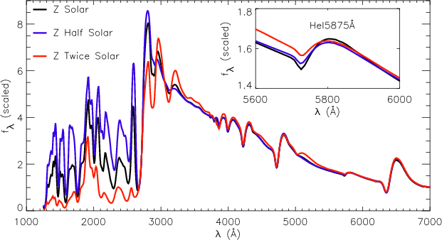 |
Figure 9:
Comparison of the emergent flux from models with identical parameters apart
from a different adopted
metallicity. The black curve describes a model with solar metal abundance.
The red (blue) shows the resulting emergent spectra when all metal abundances
are scaled by a factor of two (one half).
The model spectra beyond H |
| Open with DEXTER | |
In the text
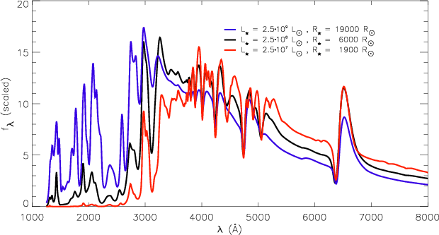 |
Figure 10:
Comparison of the emergent flux from models differing in luminosity, enhanced
and decreased by a factor of ten compared to the model in black.
Also, we scale the radius and the base density up or down by |
| Open with DEXTER | |
In the text
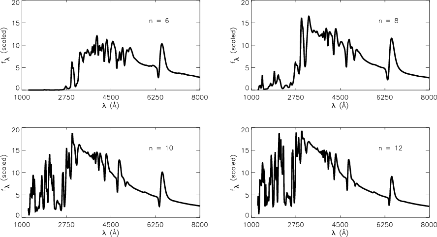 |
Figure 11: Illustration of the influence of the density exponent n on the synthetic flux distribution for n=6, 8, 10 and 12. All other model parameters are kept identical. The model atom used is small, including only the most abundant species, i.e. H I, He I, C II, N I, O I, Fe II and Fe III. |
| Open with DEXTER | |
In the text
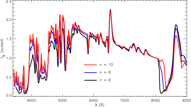 |
Figure 12: Illustration of the influence of the density exponent n on the synthetic flux distribution for n=6, 8, 10 in a cool model where hydrogen recombines near the base. All other model parameters are kept identical. Note that the most striking effect is on the set of Ca II lines near 8500 Å, the line appearing broader and stronger for smaller density exponents [color]. |
| Open with DEXTER | |
In the text
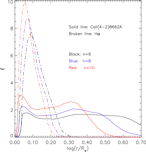 |
Figure 13:
Illustration of the relative line emission occurring at a given height in the outflow, both
for one of the three components of the Ca II feature at ca. 8500 Å,
i.e. Ca II8662 Å (solid line) and H |
| Open with DEXTER | |
In the text
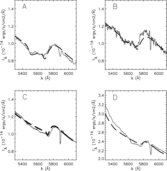 |
Figure 14:
Synthetic fits (broken line) to observations (solid line) of SN1999em
taken on the 30th of October (A), and the 1st (B), 5th (C) and 8th (D)
of November 1999 (Leonard et al. 2002a), showing the
He I 5875 Å line region.
Note how well CMFGEN manages to reproduce the observed profile using
only a modest helium enrichment over the cosmic value (
|
| Open with DEXTER | |
In the text
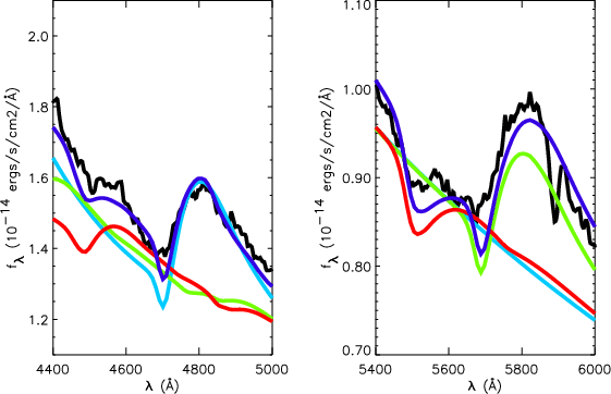 |
Figure 15: Zoom into the optical spectroscopic observations (black) of SN1999em taken on the 30th of October 1999 (Leonard et al. 2002a) showing synthetic fits for a model comprising all species as given in Table 1 (blue) or only bound-bound transitions of hydrogen (turquoise), helium (green) and nitrogen (red). We strongly support the idea that the observed features around 4600 Å and 5500 Å are due to N II lines [color]. |
| Open with DEXTER | |
In the text
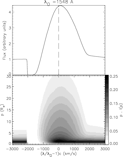 |
Figure 16:
Hot star model (WN5). Bottom: grayscale image of the
quantity
|
| Open with DEXTER | |
In the text
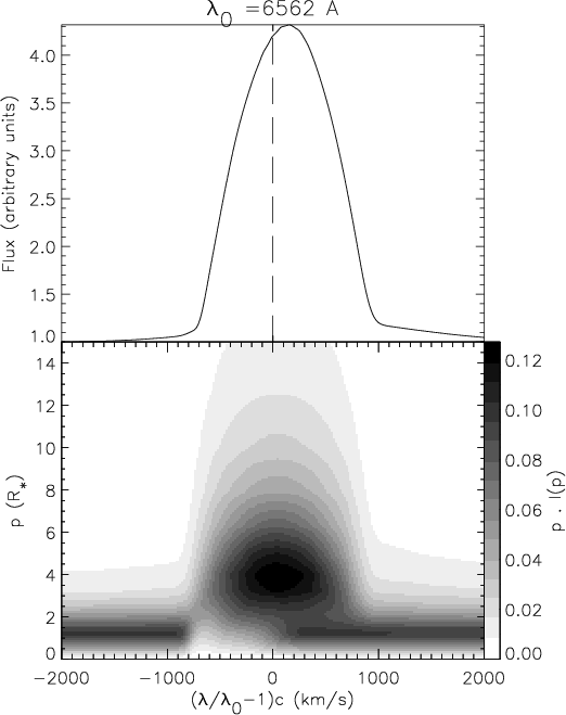 |
Figure 17:
Hot star case (WN8)
Same set as in Fig. 16 but for the H |
| Open with DEXTER | |
In the text
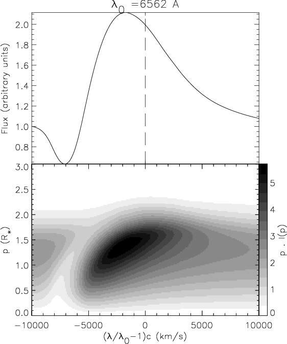 |
Figure 18:
Type II SN model
Same set as in Figs. 16 and 17
for the H |
| Open with DEXTER | |
In the text
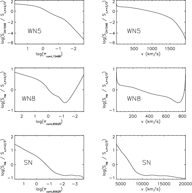 |
Figure 19:
Radial and velocity variation of the logarithm of the line source function normalized to the continuum source function at a continuum optical depth of two third (see text for details).
We show the cases corresponding to Figs. 16-18,
i.e. for C IV 1548 in the WN5 model ( top), H |
| Open with DEXTER | |
In the text
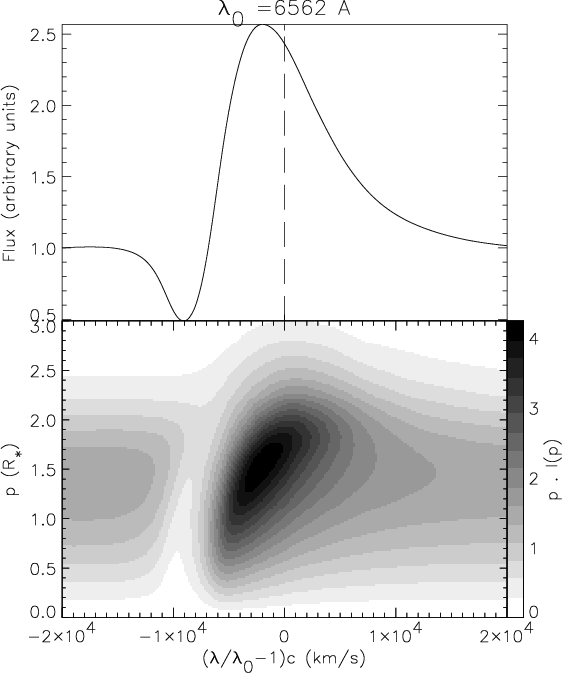 |
Figure 20: Same as Fig. 18 for a model with n=8. |
| Open with DEXTER | |
In the text
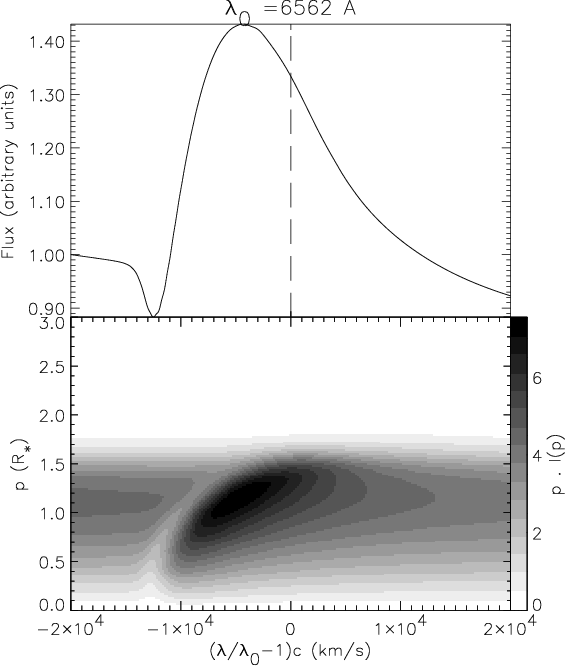 |
Figure 21: Same as Fig.18 but for a model with n=14. |
| Open with DEXTER | |
In the text