A&A 436, 1103-1111 (2005)
DOI: 10.1051/0004-6361:20042589

Particle acceleration at a three-dimensional reconnection site in the solar corona

S. Dalla - P. K. Browning

School of Physics and Astronomy, University of Manchester, PO Box 88, Manchester M60 1QD, UK

Received 21 December 2004 / Accepted 9 March 2005

Abstract
We study test particle trajectories in the vicinity of a three-dimensional (3D) magnetic null point during spine reconnection. Particles are injected into the steady-state non-uniform magnetic and electric fields derived by Priest & Titov (1996), and the equations of motion numerically integrated. We use input parameters typical of the solar corona, for which reconnection has been suggested as the fundamental mechanism responsible for particle acceleration in flare events. We show that substantial acceleration is possible in the 3D spine reconnection configuration, in the strong electric field regime. The energy gain is strongly dependent on the location of injection into the simulation box, as was the case in 2D X-point configurations. In our 3D geometry, we first vary the location of injection within a plane through the spine, and derive an analytical value for the injection angle for which maximum energy gain is achieved. Secondly we vary the azimuthal location of particle injection and show that as one moves away from the plane with maximum electric field magnitude, higher final energies can be achieved, though this requires substantially longer times.

Key words: acceleration of particles - Sun: flares - Sun: particle emission

1 Introduction

Magnetic reconnection has been put forward as an efficient mechanism for particle acceleration in a wide variety of astrophysical contexts: including the solar corona, during flares, which is the primary interest here, but also the Earth's magnetotail and pulsars (de Gouveia et al. 2000). Ions accelerated by reconnection have also been recently observed in a high temperature laboratory plasma device (Helander et al. 2002). The presence and properties of such high energy particles constitute an important diagnostic of reconnection, and the energy of non-thermal particles is a significant component of solar flare energy balance. Recent observational evidence from the RHESSI spacecraft in particular, points towards reconnection playing a key role in solar flares (Sui et al. 2004).

For the purpose of investigating how an energetic particle population is created as a result of reconnection, the test particle approach has been widely adopted. Here the trajectories of charged particles (ions and electrons) are calculated in prescribed electromagnetic fields representative of magnetic reconnection scenarios. This then allows study of how the electric field generated during the reconnection process can energise particles, and how this process depends on the magnetic field and plasma properties. The collisionless test particle approach is valid for particles of velocity a few times larger than the thermal velocity, as they have long collisional mean free paths. It is also required that the population of such high energy particles is sufficiently small that its feedback on the electromagnetic fields can be neglected. The majority of test particle studies investigating particle acceleration during reconnection, have been carried out within a 2D framework. This involves assuming uniformity of all physical parameters along one spatial direction, which is also usually the direction of the electric field. Two-dimensional studies demonstrated that efficient acceleration can take place at X-point (also called 2D null) configurations and clarified the importance of the location of particle injection into the simulation box in determining a particle's final energy (Moses et al. 1993; Deeg et al. 1991; Vekstein & Browning 1997; Burkhart et al. 1990). The effect of adding a magnetic field component transverse to the X-point plane, parallel to the electric field, has also been widely studied (Hamilton et al. 2003; Bruhwiler & Zweibel 1992; Browning & Vekstein 2001; Mori et al. 1998; Bulanov 1980). This was a first step towards more realistic 3D geometries. Even a very weak transverse field component can have a significant effect. Other studies modelled acceleration in a current sheet configuration (Litvinenko & Somov 1993; Zharkova & Gordovskyy 2004).

In this paper we adopt a test particle approach to study particle acceleration during reconnection at a 3D magnetic null. It is useful to summarise some of the results for test particle motion in 2D X-point geometries, for comparison with the 3D results presented here. It has been shown (Vekstein & Priest 1995; Vekstein & Browning 1997; Burkhart et al. 1990) that particles are strongly magnetised at global scale if the parameter:

$$\epsilon = \frac{m_0 c^2 E_0 }{q~B_0^2 L}$$ (1)

is small, where m₀ and q are the particle's rest mass and charge, c is the speed of light, E₀ and B₀ are the electric and magnetic field magnitudes and L the size of the reconnection region. For small $\epsilon$, particle orbits are adiabatic except in a small "dissipation region'' near the null point whose size is  ${\epsilon}^{1/3} L$. Within the dissipation region, the almost unmagnetised particles are directly accelerated by the electric field, with their kinetic energy gain determined by the time taken for the magnetic field to eject them (Vekstein & Priest 1995; Burkhart et al. 1990). The acquired parallel velocity scales as  $\epsilon^{-1/3} v_{\rm E}$ where $v_{\rm E}$ is the electric drift speed (see Eq. (6)). Outside the dissipation region, Vekstein & Browning (1997) calculated particle trajectories using a guiding centre approach, and showed that significant acceleration can occur due to the interaction of strong electric drift characteristic of fast driven reconnection with field line curvature/nonuniformity. The energy gained by a particle depends on the spatial location of its injection to the reconnection region. Particles which approach most closely to the neutral line undergo the greatest acceleration.

Two-dimensional configurations are necessarily somewhat unrealistic, and three-dimensional reconnection has recently become a topic of intense investigation. This has significant qualitative differences from 2D reconnection (see, for example Priest & Forbes 2002, for a review of 3D reconnection). Particular attention has been devoted to developing magnetohydrodynamic models of the kinematics and dynamics of 3D reconnection. Reconnection in 3D does not necessarily require the presence of null points in the magnetic field, but from the point of view of particle acceleration these are the most interesting configurations. Three-dimensional magnetic null points are believed to occur frequently in the solar corona, for example during flares (Aulanier et al. 2000). Indeed, given the complex topology of the coronal field arising from photospheric flux sources of mixed polarity, null points are likely to be common.

Within a 2D model, the uniformity of the electric field along one spatial direction can lead to a very large energy gain during the time when the particle is in the low magnetic field region near the null or field reversal layer. In principle, since the region is of infinite extent in the invariant direction, particles can acquire arbitrarily large energies by moving in this direction. Here we address the question of whether 3D configurations, where the electric field has finite extent and is not spatially uniform, can also be efficient particle accelerators. There have as yet been few studies of particle acceleration in such 3D configurations. A study of trajectories in the fields output of a 3D reconnection MHD code has shown significant differences in the shape of electron spectra, compared with a 2D model (Schopper et al. 1999). Test particles in analytical model fields for 3D stationary reconnection (Craig et al. 1995) have been studied by Kobak et al. (2000), including also the effects of scattering due to turbulence in the vicinity of the null point. But the complexity of the field configurations in such studies means that a direct comparison with the better understood 2D case is difficult.

Studies of magnetic reconnection in 3D, have now clarified the structure of the plasma flow and fields in the vicinity of a 3D magnetic null (Priest & Titov 1996). Two types of reconnection have been shown to occur: spine and fan reconnection. In this paper we investigate particle acceleration in the vicinity of a 3D magnetic null for the spine reconnection scenario. A natural extension will be to consider also fan reconnection and this will indeed be done in future.

We use the 3D reconnection fields derived by Priest & Titov (1996) as the input to our calculation of test particle trajectories. These simple fields are not exact solutions of the resistive MHD equations, but are derived by means of several simplifications. Full solutions, valid both in 2D and 3D have been derived by Craig et al. (1996,1995). However it has been shown in a 2D geometry, that the simplified fields produce an energetic particle spectrum which is almost identical to the one obtained from the full reconnection solution field (Heerikhuisen et al. 2002). Hence the usage of simplified fields to study the particle acceleration problem appears to be a good first approximation. It also allows a most direct comparison with the widely studied 2D problem, so that we may understand the extent to which features of particle acceleration in 2D geometries carry over to 3D, or the extent to which 3D is fundamentally different. The aim at this stage is thus to develop a basic understanding of the trajectories of charged particles and particle acceleration in 3D reconnecting geometries, which can then be applied to more complex and realistic models in future.

Trajectories are obtained by numerical solution of the full equations of motion, as decribed in Sect. 2, for parameters typical of the solar corona. General characteristics of the 3D trajectories are described in Sects. 3 and 4, while in Sects. 5-8 we focus on the acceleration problem in a 3D scenario. Conclusions are presented in Sect. 10.

   
2 Fields configuration and trajectory code

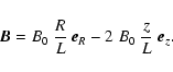
The nature of reconnection near a three-dimensional (3D) magnetic null was investigated by Priest & Titov (1996). They considered a potential 3D magnetic null, and discussed two types of reconnection which may take place in its vicinity: spine and fan reconnection. More general non-potential 3D nulls are discussed by Parnell et al. (1996) and Pontin et al. (2005).

In this study we focus on the potential 3D  magnetic null configuration, described in cylindrical coordinates $(R,\phi,z)$by the equation (Priest & Titov 1996):

$$\vec{B} = B_0 ~ \frac{R}{L} \: \vec{e}_R - 2 ~ B_0 ~ \frac{z}{L} \: \vec{e}_z.$$ (2)

Here L is the size of the reconnection region, B₀ is the magnitude of $\vec{B}$ at R=L and z=0, and $\vec{e}_R$ and $\vec{e}_z$ indicate unit vectors in cylindrical coordinates. Figure 1a shows a plot of the magnetic field lines given by Eq. (2), having cylindrical symmetry about the z axis, called the spine. In the Cartesian x-y plane, the field lines are straight lines through the null describing a fan, hence it is called the fan plane.

By imposing continous footpoint motions on a cylindrical boundary enclosing the null, Priest & Titov (1996) were able to derive analytical expressions for the electric field and flow velocity associated to 3D reconnection. For spine reconnection, footpoint motions are imposed on the curved surface of the cylindrical boundary, in such a way that field line motion takes place in planes through the spine. A plane through the spine can be characterised by the azimuthal angles $\phi, \: \phi+\pi$. The field lines approach the null point moving within such a plane, break and reconnect as the footpoints cross the plane z=0.

For fan reconnection, continuos footpoint motions are imposed on the two bases of the cylindrical boundary, causing a swirling motion of magnetic field lines at the fan.

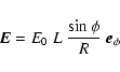
In this paper we consider the spine reconnection scenario, for which the electric field associated to reconnection takes the form (Priest & Titov 1996):

$$\vec{E} = E_0 ~ L ~ \frac{\sin{\phi}}{R} ~ \vec{e}_{\phi}$$ (3)

with E₀ the electric field magnitude at R=L and $\phi =90^{\circ }$ (value of $\phi$ for which the electric field is maximum). This field is directed along the azimuthal direction. We note that although the magnetic field is azimuthally symmetric, the electric field is not. The inflow and outflow regions for the spine reconnection configuration are shown in Fig. 1b.

We obtain particle trajectories by numerically solving the equations of motion of a particle in the magnetic and electric fields $\vec{B}$ and $\vec{E}$:

$$\frac{{\rm d} \vec{x}}{{\rm d} t} \frac{\vec{p}}{m_0 \gamma}$$ = (4)

$$\frac{{\rm d} \vec{p}}{{\rm d} t} q ~ \left( \vec{E} + \frac{1}{c} \frac{\vec{p}}{m_0 \gamma} \times \vec{B} \right)$$ = (5)

where t is time, $\vec{x}$ and $\vec{p}$ are the particle's position and momentum, q and m₀ its charge and rest mass, $\gamma$ its relativistic factor, and c is the speed of light. Here Eqs. (2), (3) are used for $\vec{B}$ and $\vec{E}$.

	Figure 1: a) Magnetic field lines for the potential 3D  magnetic null configuration. b) Diagram of the inflow and outflow regions for spine reconnection.
Open with DEXTER

The particle's equations of motion are solved numerically by means of a variable-order variable-step Adams method, as implemented in the subroutine D02CJF of the NAG libraries (NAG Fortran Library 1999). Distances are normalised by the characteristic length L, the magnetic field by B₀, and times by the nonrelativistic gyroperiod associated with a magnetic field of magnitude B₀: $T=2\pi m_0 c /(\vert q\vert B_0)$.

To verify that the numerical integration is performed accurately, we monitor the sum of kinetic and potential energy, which is a constant of motion (as described in Sect. 4). In the runs of the code described in this paper, we find that this quantity is conserved up to the first 6 significant figures. We developed both a relativistic and non-relativistic version of the code, which give identical results for a particle which does not reach relativistic energy. We use the relativistic version of the code in the next sections as near-relativistic energies are reached in the strong electric field regime as discussed below.

  
3 Weak/strong electric field regimes

A particle injected into the non-uniform fields given by Eqs. (2), (3) will follow a trajectory which depends on the field magnitudes and spatial variations, and on the initial particle position and velocity. We inject particles with a small initial energy, at a boundary of the reconnection site, i.e. at a distance L from the null point, corresponding to the dimensionless value R=1.

In regions where the particle is strongly magnetised, the motion can be described as the superposition of a rapid gyration about the local magnetic field direction and a drift motion of the guiding centre (adiabatic approximation). However near the null point this approximation breaks down as the particle becomes essentially unmagnetised (nonadiabatic region); this is where the particle can be most efficiently accelerated by the electric field.

In the adiabatic region, a particle is subject to drifts associated with the magnetic field gradient and curvature, and to the electric field drift, with velocity:

$$\vec{v}_E= c ~ \frac{\vec{E} \times \vec{B}}{B^2}\cdot$$ (6)

Two regimes of particle motion can therefore be identified based on the ratio of the initial velocity associated to the gyromotion to the electric drift velocity (Vekstein & Browning 1997). We define the parameter:

$$\tilde{\mu} = \frac{ v_{\Omega}^2 }{v_E^2}$$ (7)

where $v_{\Omega}$ is the speed associated to the gyration about the magnetic field line, and v_E the electric drift speed, given by Eq. (6). Values of $\tilde{\mu} \gg 1$ characterise a weak electric field regime, and values of order 1 or smaller a strong electric field one. The latter is characteristic of fast reconnection.

We observe that the electric field given by Eq. (3) varies as  $\sin{\phi}$, where $\phi$ is the azimuthal coordinate in the cylindrical coordinate system chosen. Therefore in the plane corresponding to the values $\phi =90^{\circ }$, 270$^{\circ }$, the electric field magnitude is maximum. Thus, for our initial studies, we focus on particles injected in this plane.

	Figure 2: Trajectories for the weak electric field ( top panels) and strong electric field ( bottom panels) regimes. The particle's initial position is (x0,y0,z0)=(0, 0.8, 0.6), and input parameters are given in Table 1. Dotted lines indicate projections of magnetic field lines.
Open with DEXTER

Table 1: Input parameters to the trajectory code for runs of Fig. 2.

Figure 2 shows the trajectories of a proton for two values of the electric field magnitude. For each case the trajectory is described by its projections along the x-y plane (the fan plane) and the y-z plane, the z axis being the spine. Dotted lines represent projections of magnetic field lines. The top panels of Fig. 2 are for E₀=30 V/m, and the bottom panels for E₀=1.5 kV/m. In the former case $\tilde{\mu}=4100$ and we are in the weak electric field regime, in the latter case $\tilde{\mu}=1.5$ and we are just in the strong electric field regime. The other input parameters for the numerical integration are summarised in Table 1. The magnetic field strength is typical of the solar corona. The length scale is small compared with the observed size of coronal structures (e.g. a flare region) because the model fields here are supposed to apply to a localised reconnection site within a global field configuration - thus the length L is the scale on which the fields near a null can locally be approximated by Eqs. (2), (3). The electric field cannot be easily determined from observations. Whilst the value for the "strong electric field'' regime might appear large, it should be noted that this is only expected to exist in a localised region, and indeed we expect such strong fields (giving values of  $\tilde{\mu}$ near 1) for fast reconnection with inflow speed a significant fraction of the Alfvén speed. The particle is injected at a position (x₀,y₀,z₀)=(0, 0.8, 0.6) hence in the plane where the electric field is maximum. Thus for this choice of parameters the values of $\epsilon$, as given by Eq. (1), are $\epsilon=0.30\times 10^{-6}$ for the weak electric field regime and $\epsilon=0.15\times 10^{-4}$ for the strong electric field one.

In the weak electric field case, the particle is spiralling about the magnetic field line (this component of the motion not being visible in Fig. 2 as the gyroradius is much smaller than the lenght scale L), and its velocity reverses at mirror points as a result of the nonuniformity of the magnetic field. The simulation is run up to a final dimensionless time of 320 000 (gyroperiods), corresponding to a dimensional final time of 2 s. The particle is not accelerated, its final energy being 250 eV.

In the strong electric field case, however, a large acceleration is observed, with the proton reaching 0.9 MeV after a time of 10 000 (gyroperiods) corresponding to 65 ms. The presence of two separate regimes of particle motion depending on the value of the electric field and the corresponding dimensionless parameter  $\tilde{\mu}$, as shown in Fig. 2, is similar to what is observed in 2D configurations (Vekstein & Browning 1997).

   
4 Energy conservation

We now introduce a potential for the electric field and calculate the sum of kinetic and potential energy for our system. This quantity remains constant during the motion.

A potential V such that $\vec{E}=-\nabla V$ can be obtained from Eq. (3), and is given by:

$$V(\phi)= E_0 ~ L ~ \cos{\phi} .$$ (8)

Conservation of energy implies that the quantity W, given by

$$W = K + q V = K + q~ E_0 ~ L ~ \cos{\phi}$$ (9)

where K is the kinetic energy, is conserved during the motion. The kinetic energy can be derived from the momentum by means of the equation:

$$K=\sqrt{c^2p^2+m_0^2 c^4} - m_0~ c^2$$ (10)

which reduces to K=1/2  m₀ v² in the nonrelativistic case.

Equation (9) implies that 2   q   E₀ L is the maximum kinetic energy which can be gained by a particle in this configuration. A particle may or may not gain this maximum energy, depending on the details of its trajectory. For a particle with initial kinetic energy negligible compared to q   E₀ L, the kinetic energy at a time twill be given by:

$$K(t)=q ~ E_0 L (\cos{\phi_0} - \cos{\phi(t)})$$ (11)

where $\phi_0$ is the azimuthal angle at t=0. This equation implies that for a positive particle starting with $\phi_0 \in [0,\pi/2]$, acceleration will be associated with a decrease of  $\cos{\phi}$during the motion, i.e. counterclockwise motion. The opposite will be true for a negatively charged particle. For the strong electric field regime of Table 1, the quantity 2   q   E₀ L, i.e. the maximum possible kinetic energy gain is  $3.0\times 10^7$ eV.

   
5 Dependence of energy gain on initial position

Figure 3: Dependence of energy gain on the particle's initial position. Top panel: each line type represents a particle trajectory projected onto the y-z plane. Bottom panel: time variation of the kinetic energy for the trajectories shown in the top panel. Here time is normalised by the initial particle gyroperiod. We consider a proton of initial energy 300 eV and initial pitch-angle 92$^{\circ }$, other parameters as in Table 1, for the strong electric field regime.

Open with DEXTER

We now focus on the strong electric field regime, and study how the energy gain depends on the particle's initial position. We will show that the energy gain strongly depends on the location where the particle is injected into the box, and that the largest energy gain is associated to locations where the electric field drift, with velocity given by Eq. (6), takes the particle very close to the magnetic null, where acceleration is most efficient.

In the case of spine reconnection, $\vec{v}_E$ lies in planes through the spine, hence we focus first on one such plane, the y-z plane. Here $\phi =90^{\circ }$ and the electric field is maximum. It might be expected that particles injected in this plane are most strongly accelerated, though we shall see later in Sect. 8 that this is not in fact the case.

The dependence of the final energy on initial positions in the y-z plane is shown in Fig. 3, where different line types correspond to different initial positions on the circle of radius R=1. Other parameters such as the particle's initial energy and pitch angle and the configuration of the fields are kept constant. For the dashed trajectory (a), the particle drifts quickly towards the spine, where the electric field is strong, and is efficiently accelerated. The solid trajectory (b) shows a particle going very close to the null and gaining large energy. The particle following the dash-dotted trajectory (c) however does not enter the region of strong electric field and has a much smaller energy gain.

If we introduce the angle $\beta$, giving the angle in the y-z plane between the y axis and the radius connecting the initial position to the origin, we can plot the final energy versus $\beta$, and obtain the plot given in Fig. 4. This shows the existence of an optimal angle  $\beta_{\rm opt}$ for which the particle gains the largest final energy. For angles smaller than  $\beta_{\rm opt}$, the energy gain drops quickly, corresponding qualitatively to the (c) trajectory of Fig. 3. For angles larger than $\beta_{\rm opt}$, large acceleration can be obtained, corresponding to trajectories such as (a) in Fig. 3.

The 3D result shown in Fig. 4 can be compared with results previously obtained in a 2D X-point configuration (Vekstein & Browning 1997), keeping in mind that the magnetic field lines in Fig. 1 of the latter reference need to be rotated by 45 degrees about the origin, to display a dependence similar to that of 3D field lines in a plane through the spine. In a 2D configuration, the optimal angle of approach is 45$^{\circ }$ and there is symmetry about the line of optimal approach. In a 3D geometry we obtain a smaller optimal angle, and as shown in Fig. 4, there is no symmetry about the line of optimal approach.

	Figure 4: Plot of the particle's final energy versus the angle $\beta$ characterising the initial position in the y-z plane. Points are for a proton of initial energy 300 eV and initial pitch-angle 90$^{\circ }$, and other parameters as in Table 1, for the strong electric field regime.
Open with DEXTER

The value of the angle $\beta_{\rm opt}$ can be obtained analytically by calculating the expression of the flow lines of the velocity  $\vec{v}_{\rm E}$, from Eq. (6) combined with Eqs. (2) and (3). One obtains that flow lines are described by:

R²= 2   z² + C (12)

where C is a constant. This shows that flow lines through the magnetic null exist, corresponding to C=0 and described by the equation:

$$R= \sqrt{2} ~ \vert z\vert .$$ (13)

A particle with initial position on one of these flow lines, inside an inflow region, and with pitch-angle 90$^{\circ }$ ( $v_{\perp}=0$), will go very close to the magnetic null and will be accelerated with highest efficiency. From Eq. (13), the angle formed with the y axis by the flow line through the origin is $\beta_{\rm opt}=\tan^{-1}(1/\!\sqrt{2})=35.3^{\circ}$. This analytical value of  $\beta_{\rm opt}$ is in agreement with the numerical value obtained from runs of the trajectory code, as can be seen from Fig. 4.

6 Pitch-angle dependence

	Figure 5: Trajectories in the y-z plane for the same initial conditions as trajectory (b) of Fig. 3, but different values of the initial particle pitch-angle: (a) pitch-angle = 110$^{\circ }$ and (b) pitch-angle = 80$^{\circ }$.
Open with DEXTER

	Figure 6: Trajectory of a particle injected into a strong electric field configuration, with the same initial parameters as the solid-line trajectory of Fig. 3, except for the fact that initial pitch-angle is 90$^{\circ }$ rather than 92$^{\circ }$. Note that the scale of the plot is enlarged compared to that of Fig. 3.
Open with DEXTER

In the strong electric field regime, varying the value of the initial particle pitch-angle will result in very different trajectories. This is shown in Fig. 5, where the same initial conditions as for trajectory (b) of Fig. 3 were used, apart from the value of initial pitch-angle. The solid trajectory corresponds to initial pitch-angle equal to 110$^{\circ }$ and the dash-dotted one to initial pitch angle 80$^{\circ }$. It is clear that varying the initial pitch angle by as little as 10$^{\circ }$results in the particle following very different paths, and in the case of pitch angle 80$^{\circ }$ gaining much smaller energy, for injection at this particular location. A particle of pitch-angle 80$^{\circ }$ will however be able to gain large energy if injected at a larger value of $\beta$, in such a way that it passes close to the null point. In other words, a plot similar to the one shown in Fig. 4 can be obtained for any pitch angle, with the position of the peak (i.e. the optimal injection angle) being different for different pitch angles.

7 Chaotic orbits

It is well known that magnetic null configurations can give rise to chaotic orbits, since the Larmor radius diverges where the magnetic field becomes zero (Nocera et al. 1996). Figure 6 shows the trajectory of a proton in the strong electric field regime, with the same initial position and very similar initial velocity as the solid-line trajectory of Fig. 3. The only parameter that was changed in this run with respect to the one in Fig. 3 is the initial pitch-angle, which is here 90$^{\circ }$ rather than 92$^{\circ }$. Thus the particle moves directly towards the null, initially along the drift streamline given by Eq. (13).

This small change in the initial conditions results in the particle following a completely different trajectory, an indication of chaotic behaviour. This type of behavior is observed only for trajectories going very close to the magnetic null.

   
8 Varying the plane of injection

In Sects. 3 and 5 we injected particles into the simulation box at various locations in the plane $\phi =90^{\circ }$, where the value of the electric field at a distance R=1 from the spine is largest.

	Figure 7: Top panels: trajectories for injections at different values of $\phi$, i.e. for initial positions is in the semiplanes: (a):  $\phi =90^{\circ }$; (b):  $\phi =55^{\circ }$; (c):  $\phi =20^{\circ }$; bottom panel: time variation of the kinetic energy for the three trajectories.
Open with DEXTER

We now consider trajectories with initial positions in other planes, characterised by a value of $\phi$ different from 90$^{\circ }$and consequently electric fields at R=1 smaller than the values previously considered.

In Fig. 7 the trajectory (a) is for a particle injected in the semiplane with $\phi =90^{\circ }$ where the electric field is maximum, trajectory (b) for a particle injected in the semiplane $\phi =55^{\circ }$, with a smaller value of the initial electric field, and (c) for $\phi =20^{\circ }$, where the initial electric field is 0.34 times the value in the plane  $\phi =90^{\circ }$. The bottom panel shows the variation of kinetic energy with time for the three trajectories. We see that a particle moving initially in a plane with smaller electric field takes a longer time to reach the region where acceleration is most efficient, as a result of the electric drift speed being smaller. However, it gains a larger final energy.

We therefore have the surprising result that the plane with maximum electric field is not the one where the largest kinetic energy is gained. This fact can be understood in terms of the energy conservation arguments presented in Sect. 4, in the sense that, from Eq. (11), the value of $\cos{\phi_0}$, where $\phi_0$ is the azimuthal angle at t=0, influences the maximum energy that can be reached by a particle. For all three trajectories in Fig. 7, particles exit the reconnection region near $\phi=270^{\circ}$, where  $\cos{\phi}$, the second term on the rhs of Eq. (11), is small. For trajectory (b), the initial potential energy (first term on the rhs of Eq. (11)), is $q~ E_0 ~ L ~ \cos{\phi_0}= 8.6\times 10^6$ eV, and this is approximately the energy gained during the motion. A similar behaviour is seen for trajectory (c) for which initially $q~ E_0 ~ L ~ \cos{\phi_0}= 2.8\times 10^7$ eV, allowing an even larger acceleration. For the trajectory (a), $q~ E_0 ~ L ~ \cos{\phi_0}= 0$, hence the magnitude of the energy gain is determined by $q~ E_0 ~ L ~ \cos{\phi(t)}$at the time of exit from the acceleration region, and this is about an order of magnitude smaller than in previous cases as $\phi$ is close to 270$^{\circ }$. In all three cases motion in the region near the null is towards decreasing values of  $\cos{\phi}$, i.e. in the counterclockwise direction.

The plane with maximum electric field ( $\phi =90^{\circ }$) is the one where a particle takes the shortest time to arrive in the vicinity of the null, as a result of $v_{\rm E}$ being large. In other words, acceleration happens on the shortest time scales in this plane. Figure 7 shows that as one moves to smaller values of $\phi$, the time required for a particle to be strongly accelerated increases, becoming for the plane $\phi =20^{\circ }$ more than 3 times larger than for the plane $\phi =90^{\circ }$. For values of $\phi$ below  $20^{\circ}$ a situation is reached where the electric drift velocity $v_{\rm E}$ becomes smaller than other drift velocities and the particle does not reach the region near the null, inhibiting efficient acceleration.

As noted above, for all three trajectories in Fig. 7 particles exit the region near the null at an angle close to $\phi=270^{\circ}$. This shows a tendency of accelerated particles to be focussed near the plane where the electric field is maximum. It should be however pointed out that, for the parameters considered in Fig. 7, particles moving away from the null become trapped by the magnetic field, and start bouncing back and forward in the way shown in Fig. 8, which displays the trajectory (c) of Fig. 7 up to longer times.

	Figure 8: Trajectory for injection in the plane $\phi =20^{\circ }$, integrated over a longer time than in Fig. 7. Here $t_{\rm final}=13~000.$
Open with DEXTER

The behaviour shown in Fig. 8 is the result of the particle having gained a large energy: once it exits the region near the null, the value of  $\tilde{\mu}$, as defined by Eq. (7), has now become very large, i.e. the electric field drift is not the dominant component of the motion, as it was prior to passage by the null point.

	Figure 9: Top panels: trajectories for injections into the electric field given by Eq. (14), with three values of  $L_{\rm sp}$. The plot for $L_{\rm sp}=0$ is the same as trajectory (b) of Fig. 7.
Open with DEXTER

9 Singularity at the spine

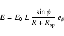
The electric field and flow velocity given by Eqs. (3) and (6) respectively, were derived by Priest & Titov (1996) within the ideal MHD description, and are therefore valid outside the region close to the spine where resistive effects need to be taken into account. As a result the electric field displays a 1/R dependence, i.e. a singularity at the spine. It was shown by Priest & Titov (1996) that resolution of this singularity cannot be achieved within linear MHD theory, and that a fully non-linear resistive treatment is required to eliminate it. While a solution to the latter resistive MHD problem is being worked out by scientists, the qualitative effect of the removal of the singularity at spine on energetic particle trajectories can be studied by considering a modified electric field of the following form:

$$\vec{E} = E_0 ~ L ~ \frac{\sin{\phi}}{R + R_{\rm sp}} ~ \vec{e}_{\phi}$$ (14)

where $R_{\rm sp}$ represents the typical radius in cylindrical coordinates of the region where resistive effects need to be taken into account.

We injected particles into a configuration with modified electric field given by Eq. (14), and studied how the resolution of the singularity at the spine would impact the results on particle acceleration presented in the previous sections.

We considered two values of the dimensionless parameter $L_{\rm sp}=R_{\rm sp}/L$, given by $L_{\rm sp}=0.001$ and  $L_{\rm sp}=0.01$, and compared trajectories for these two cases with the one obtained by using the original singular electric field, i.e. $L_{\rm sp}=0$. The corresponding trajectories are shown in Fig. 9. One can observe that for $L_{\rm sp}=0.001$, the trajectory and energy gain are very similar to the $L_{\rm sp}=0$ case. However for a value $L_{\rm sp}=0.01$, there are large differences in the trajectory and in the energy gained by a particle, although the particle is still accelerated in this case.

We conclude that the size of the non-ideal region around the spine is an important parameter in determining the magnitude of the energy gained by a particle, and that quantitative application of the results described in this paper would require the size of the resistive region to be orders of magnitude smaller than the entire region under consideration.

   
10 Conclusions

We obtained trajectories of particles near a 3D magnetic null during spine reconnection, and studied the dependence of the energy gain on the field properties and the particle's initial position. Particles injected from the boundaries of a supposed localised reconnection site were investigated, with a range of injection positions.

We found that efficient particle acceleration can take place in the strong electric field regime which is expected in fast magnetic reconnection. The energy gain is strongly dependent on the initial position of the particle. Within a plane passing through the spine, an optimal angle above (or below) the fan plane exists, for which maximum acceleration is observed. This angle is found to be $\beta_{\rm opt}=35.3^{\circ}$, for a particle of pitch angle 90$^{\circ }$. This is broadly consistent with studies of 2D configurations, although the "symmetry breaking'' of moving to 3D means that this optimal angle is no longer a simple 45$^{\circ }$.

We also studied the acceleration of particles injected in different planes through the spine, i.e. we considered several values of the azimuthal coordinate $\phi$ for the initial position, as the electric field in spine reconnection has a $\sin{\phi}$ dependence. We found that particles injected at an angle to the plane where the electric field is maximum can also be very efficiently accelerated, though it takes a longer time. Surprisingly, the initial position which gives the greatest net kinetic energy gain is not that at which the electric field is strongest. An interesting feature, which could be significant in terms of interpreting observations of accelerated particles, is that the particles do not leave the reconnection site isotropically distributed in direction, but tend to exit the reconnection region along a preferred direction.

Since the study of particle trajectories in 3D null point configurations is quite novel, our work is quite preliminary and can be extended naturally in future in a number of ways. A first step, as previously mentioned, will be to investigate also fan reconnection. Furthermore, within the same configuration, the trajectories of electrons and ions can be quite different due to the different charge to mass ratio; this has been recently emphasised by Zharkova & Gordovskyy (2004), who provide an explanation of flare observations in terms of proton-electron separation due to acceleration in a 2D current sheet. Thus, in future we will analyse the dependence of trajectories on the charge to mass ratio of particles, considering electrons as well as different ion species. Energy spectra, and their dependence on the angle of the ejected particles, will be calculated. These results will be compared with observations e.g. from the RHESSI spacecraft. It is also important to note that the null point geometry considered here is only a special case, and in future more general 3D null points will be investigated (Parnell et al. 1996).

Our model does not include the effects of inductive electric fields generated by the strong transient currents likely to be present in many reconnection scenarios such as in solar flares, and this will be the subject of future study.

Acknowledgements

S.D. acknowledges support from the UK Particle Physics and Astronomy Research Council through a Post-Doctoral Fellowship.

References

• Aulanier, G., DeLuca, E. E., Antichos, S. K., McMullen, R. A., & Golub, L. 2000, ApJ, 540, 1126 [NASA ADS] [CrossRef] (In the text)
• Browning, P. K., & Vekstein, G. E. 2001, J. Geophys. Res., 106, 18677 [NASA ADS] [CrossRef]
• Bruhwiler, D. L., & Zweibel, E. G. 1992, J. Geophys. Res., 97, 10825 [NASA ADS]
• Bulanov, S. V. 1980, Sov. Astron. Lett. 6, 206
• Burkhart, G. R., Drake, J. F., & Chen, J. 1990, J. Geophys. Res., 95, 18833 [NASA ADS]
• Craig, I. J. D., & Fabling, R. B. 1996, ApJ, 462, 969 [NASA ADS] [CrossRef]
• Craig, I. J. D., Fabling, R. B., Henton, S. M., & Rickard, G. J. 1995, ApJ, 455, L197 [NASA ADS] (In the text)
• Deeg, H.-J., Borovsky, J. E., & Duric, N. 1991, Phys. Fluids B, 3, 2660 [NASA ADS] [CrossRef]
• de Gouveia dal Pino, E., & Lazarian, A. 2000, ApJ, 536, L31 [NASA ADS] [CrossRef] (In the text)
• Hamilton, B., McClements, K. G., Fletcher, L., & Thyagaraja, A. 2003, Sol. Phys., 214, 339 [NASA ADS] [CrossRef]
• Heerikhuisen, J., Litvinenko, Y. E., & Craig, I. J. D. 2002, ApJ, 566, 512 [NASA ADS] [CrossRef] (In the text)
• Helander, P., Eriksson, L.-G., Akers, R. J., et al. 2002, Phys. Rev. Lett., 89, 235002 [NASA ADS] [CrossRef] (In the text)
• Kobak, T., & Ostrowski, M. 2000, MNRAS, 317, 973 [NASA ADS] [CrossRef] (In the text)
• Litvinenko, Yu. E., & Somov, B. V. 1993, Sol. Phys., 146, 127 [NASA ADS] [CrossRef]
• Mori, K.-I., Sakai, J. I., & Zhao, J. 1998, ApJ, 494, 430 [NASA ADS] [CrossRef]
• Moses, R. W., Finn, J. M., & Ling, K. M. 1993, J. Geophys. Res., 98, 4013 [NASA ADS]
• NAG Fortran Library Manual 1999, Mark 19, NAG Ltd. (In the text)
• Nocera, L., Pegoraro, F., Bulanov, S. V., & Bertin, G. 1996, Phys. Scr., T63, 197 [NASA ADS] (In the text)
• Parnell, C. E., Smith, J. M., Neukirch, T., & Priest, E. R. 1996, Phys. Plasmas, 3, 759 [NASA ADS] [CrossRef] (In the text)
• Pontin, D. I., Hornig, G., & Priest, E. R. 2005, Geophys. Astrophys. Fluid Dynamics, 99, 77 [NASA ADS] (In the text)
• Priest, E. R., & Titov, V. S. 1996, Phil. Trans. R. Soc. Lond. A, 354, 2951 (In the text)
• Priest, E. R., & Forbes, T. G. 2002, Magnetic Reconnection (Cambridge University Press) (In the text)
• Schopper, R., Birk, G. T., & Lesch, H. 1999, Phys. Plasmas, 6, 4318 [NASA ADS] [CrossRef] (In the text)
• Sui, L., Holman, G. D., & Dennis, B. R. 2004, ApJ, 612, 546 [NASA ADS] (In the text)
• Vekstein, G. E., & Priest, E. R. 1995, Phys. Plasmas, 2, 3169 [NASA ADS] [CrossRef]
• Vekstein, G. E., & Browning, P. K. 1997, Phys. Plasmas, 4, 2261 [NASA ADS] [CrossRef]
• Zharkova, V., & Gordovskyy, M. 2004, AJ, 604, 884 [NASA ADS] [CrossRef]