A&A 435, 1159-1167 (2005)
DOI: 10.1051/0004-6361:20041596
Coronal loops heated by turbulence-driven Alfvén waves:
A two fluid model
I. O'Neill
- X. Li
Institute of Mathematical and Physical Sciences, University of Wales, Aberystwyth, SY23 3BZ, UK
Received 5 July 2004 / Accepted 8 February 2005
Abstract
We present the results of a thorough parameter study of coronal loop models in the aim to explore the mechanism behind coronal heating. The two-fluid coronal loops described in this paper have lengths from 10 Mm to 600 Mm and consist of protons and electrons. The loops are treated with our unique, self-consistent, steady state dynamic loop model to derive the basic parameters (as introduced by Li & Habbal 2003, ApJ, 598, L125). The only heating mechanism assumed is turbulently generated Alfvén waves that carry the necessary flux from the chromosphere to energize the coronal plasma through preferential heating of the proton gas. Strong Coulomb coupling allows energy to pass efficiently from protons to electrons. We have control over the independent variables, driving scale (l) and Alfvén amplitude ( ), which influence the dissipation and flux of these resonant waves. We find "mapping'' the loop parameter response to varying l with fixed
a useful tool to find where certain conditions for each loop length exist. From this, we are able to pin-point where the coldest solution lies. For a loop of L=10 Mm, the coolest loops have a maximum temperature of T=0.75 MK. We also focus on a L=40 Mm loop and vary both l and
so we can compare results with existing work. From this parameter mapping we can categorise the loop heating profiles. Our model indicates the existence of footpoint, non-uniformly and quasi-uniformly heated profiles. There is also strong evidence to suggest the same mechanism may apply to hot, SXT loops.
), which influence the dissipation and flux of these resonant waves. We find "mapping'' the loop parameter response to varying l with fixed
a useful tool to find where certain conditions for each loop length exist. From this, we are able to pin-point where the coldest solution lies. For a loop of L=10 Mm, the coolest loops have a maximum temperature of T=0.75 MK. We also focus on a L=40 Mm loop and vary both l and
so we can compare results with existing work. From this parameter mapping we can categorise the loop heating profiles. Our model indicates the existence of footpoint, non-uniformly and quasi-uniformly heated profiles. There is also strong evidence to suggest the same mechanism may apply to hot, SXT loops.
Key words: Sun: corona - Sun: transition region
It is well known that the lower corona is a highly dynamic and diverse region of the solar environment. Observations by the Transition Region and Coronal Explorer (TRACE), Solar and Heliospheric Observatory (SOHO) and Yohkoh (Soft X-ray Telescope, SXT) have shown there to be a zoo of coronal structures, that vary in scale, lifetime, variability and luminosity. The revolutionary spatial and temporal resolution of TRACE has given us a unique insight to the coronal heating phenomena and the nature of these elegant structures. Although advanced observational data is becoming available, the mechanisms behind the observed coronal heating are poorly understood. For instance, recent observations revealed that EUV loops have flat temperature profiles (Lenz et al. 1999). It is known that the majority of these loops cannot be explained by assuming hydrostatic equilibrium, especially long coronal loops (Winebarger et al. 2002; Ashwanden et al. 2001; Klimchuk 1987), when compared with classical models (Rosner et al. 1978). This is because the observed loops can be several orders of magnitude denser (and brighter) than values expected from hydrostatic models (Winebarger et al. 2003). Steady flows have been detected (Winebarger et al. 2002) and have led to speculation that steady flow may be the answer to these observed "overdense'' loops. More recently however, Patsourakos et al. (2004) demonstrated that a steady plasma flow fails to explain the flat temperature profile and high density for a 300 Mm loop. Further work is obviously needed.
A possible way to enhance the density in coronal loops is momentum deposition by plasma waves. Litwin & Rosner (1998) suggested that Alfvén waves can increase the coronal scale heights and therefore coronal loop densities. Recently, Li & Habbal (2003) developed a coronal heating model that simulates the dissipation of Alfvén waves propagating from one footpoint (at s=0) to the other (s=L) due to a fully developed turbulent cascade. The model is successful in producing steady flows, flat coronal temperatures and high electron densities. However, the model is only applied to a relatively short loop (L=70 Mm).
The purpose of this paper is to apply the model developed by Li & Habbal (2003) and Li et al. (2004) to various loops. This is a thorough parameter study to explore the coronal response to this mechanism in various conditions. We study Alfvén waves as they carry a large energy flux due to the high Alfvén velocity in the corona. Studies by Hara & Ichimoto (1999) and other authors strongly imply that Alfvén waves may be present in observational data of coronal loops and play a key role in coronal heating. We therefore simulate asymmetric plasma flow (Noci & Zuccarello 1983; Craig & McClymont 1986) with Alfvén wave dissipation acting as the driving force.
The chromosphere acts as a reservoir of plasma as one footpoint "drains'' matter into the corona. The photospheric environment is such that it provides a very efficient connection between the sub-photospheric magnetic field and coronal loops (line-tied) as the high mass density and high conductivity provide a very efficient anchor. Oscillations within the solar body are then readily transmitted through the loop structure. We assume the power spectrum of waves transmitted is maintained by a non-linear turbulent cascade where Alfvén waves interact non-linearly to increase the overall wave frequency, maintaining the wave dissipation through the body of the loop. Observations of non-thermal motions in the corona are attributed to such MHD disturbances (Chae et al. 1998).
2 The model and method
We simulate a thin semi-circular cylindrical tube (of length  )
of magnetic flux projecting from the solar "surface'' (photospheric footpoints), through the transition region and into the corona. The gravitational acceleration will therefore vary along the axis of the cylinder. The tube is assumed to consist of bundled small-scale "fibrils'' (as observed by the high resolution of TRACE) which channel the flow of plasma from one footpoint to the other. Using a full-implicit scheme for a one-dimensional model (Hu et al. 1997), the simulation is allowed to attain steady state before results can be taken. The basic one-dimensional, time dependent equations are summarised from Eqs. (1) to (7).
)
of magnetic flux projecting from the solar "surface'' (photospheric footpoints), through the transition region and into the corona. The gravitational acceleration will therefore vary along the axis of the cylinder. The tube is assumed to consist of bundled small-scale "fibrils'' (as observed by the high resolution of TRACE) which channel the flow of plasma from one footpoint to the other. Using a full-implicit scheme for a one-dimensional model (Hu et al. 1997), the simulation is allowed to attain steady state before results can be taken. The basic one-dimensional, time dependent equations are summarised from Eqs. (1) to (7).
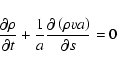
The time dependent continuity equation can be written as
 |
(1) |
where  is the plasma mass density (
 as
as
 ), v is the plasma velocity, a is the loop cross section (assumed to be constant) and s is the position along the axis of the loop.
The momentum equation can be written as
 |
(2) |
where  ,
,
 and
and  are the electron, proton and turbulent wave pressure respectively and g|| is the gravitational component acting on the plasma. g|| is expected to have a maximum deceleration (acceleration) effect on upflowing (downflowing) plasma. Naturally, g||=0 at the loop apex. Our model is unique in that Alfvén waves are used. These waves will introduce momentum deposition to the loop plasma. Momentum deposition may play a very important role in pulling plasma from the chromosphere to the corona (Li & Habbal 2003).
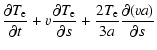
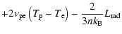
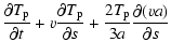
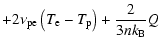
The electron and proton energy equations can be written as
where  and
and  are the electron and proton temperatures, n is the plasma density (plasma quasi-neutrality applies,
 ),
),  is the Boltzmann constant,
 and
and
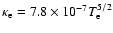
 are the collision-dominated electron and proton heat flux conductivities (
 ,
,
 ; Spitzer 1962).
 is the radiative energy loss from the loop (for an optically thin plasma as derived by Rosner et al. 1978). This parameter is strongly influenced by the density of electrons. Q however is the heating rate of the dissipating wave, energy is absorbed by the proton gas and emitted by the electron gas. Q can be of the form (Hollweg 1986)
 |
(5) |
where
is the Alfvén wave amplitude and l is the driving scale of the Alfvén waves. We will work under the assumption that the non-thermal velocities (i.e. particle motion that is not thermal in origin) observed by Chae et al. (1998) is the fingerprint of . Chae et al. found that spectral lines observed in the transition region and corona (by the Solar Ultraviolet Measurement of Emitted Radiation, SUMER, on board SOHO) exhibit excess broadening of spectral lines beyond thermal broadening. The temperatures analysed in this study range from
 K to 106 K and the corresponding non-thermal velocities
(or )
range from 5 km s-1 to 30 km s-1. We use the
vs. temperature curve for quiet-Sun disk observations plot in Fig. 5 from Chae et al. (1998) to read off the desired temperature and corresponding value of
K to 106 K and the corresponding non-thermal velocities
(or )
range from 5 km s-1 to 30 km s-1. We use the
vs. temperature curve for quiet-Sun disk observations plot in Fig. 5 from Chae et al. (1998) to read off the desired temperature and corresponding value of
 is the Coulomb collision frequency given by (Braginski 1965)
![\begin{displaymath}
\nu_{{\rm pe}}=\frac{16\sqrt{\pi}}{3}\frac{ne^{4}\ln{\Lambda...
...\frac{2k_{{\rm B}}T_{{\rm e}}}{m_{{\rm e}}}\right]^{-3/2}\cdot
\end{displaymath}](/articles/aa/full/2005/21/aa1596-04/img36.gif) |
(6) |
As the Debye length is small in lower coronal regions ( 1cm; Lenz 1999),
 becomes an important parameter as a mechanism to transport energy from protons (energized by resonant Alfvén waves) to the lower mass electrons.
 is the Coulomb logarithm (
 in this study as the lower corona is considered to be collision dominated).
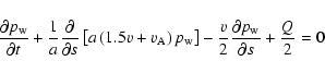
Finally, the Alfvén wave energy equation can be written as
 |
(7) |
where
is the turbulent pressure (given by
 )
and
)
and  is the Alfvén speed in the medium (given by
 ).
).
All of the above continuity, momentum and energy equations are solved simultaneously to find steady state solutions.
It is important that a total overview is acquired of the response of this range of loop lengths for different Alfvén amplitudes ()
and driving scales (l; with reference to Eq. (5)). Rather than taking "shots in the dark'' and guessing at the parameters that are outputted, the maximum temperature (
 ), minimum density (
 ), maximum velocity (
 )
and minimum pressure (
)
and minimum pressure (
 )
are plotted for many steady solutions to the
and l independent variables.
)
are plotted for many steady solutions to the
and l independent variables.
This portion of our work will take on 3 sections. As an extension to Li & Habbal (2003), we analyse the response of a number of different coronal loop lengths (from a "short'' 10 Mm to a "long'' 600 Mm) to the variables
and l. The first section demonstrates the sensitivity of loop length to a range of driving scales (
l=10-8000 km) whilst being held at a constant Alfvén wave amplitude ( km s-1; corresponding to a footpoint temperature of 20 000 K; Chae et al. 1998). The second section again plots L against l, but the Alfvén amplitude is increased to
  km s-1 (corresponding to a footpoint temperature of approximately 30 000 K). The results of km s-1 can be compared with km s-1. In the third section, we focus on one loop length (L=40 Mm) to find the parameter response to both
and l variables. It is hoped by "mapping''
,
,
and
,
comparisons can be made with the results of other authors (i.e. Winebarger et al. 2003, ran tests on a L=40 Mm loop and compared their dynamic model results with observation).
km s-1 (corresponding to a footpoint temperature of approximately 30 000 K). The results of km s-1 can be compared with km s-1. In the third section, we focus on one loop length (L=40 Mm) to find the parameter response to both
and l variables. It is hoped by "mapping''
,
,
and
,
comparisons can be made with the results of other authors (i.e. Winebarger et al. 2003, ran tests on a L=40 Mm loop and compared their dynamic model results with observation).
As the flux and speed of wave dissipation is changed from one solution to the next, the heating profile is unique for each steady solution computed. The following heating profiles are evident in the data described above:
- a)
- Quasi-uniform heating. Wave energy is slowly dissipated, allowing some heating but maintaining a very low plasma flow speed. This solution produces a quasi-uniform heated loop and a symmetrical temperature profile. Uniform heating can only be achieved with our model if the plasma velocity is non-zero, but still very small.
- b)
- Non-uniform heating. Wave energy dissipates quicker, leading to moderate heating and faster flow speeds. The temperature profile becomes asymmetric and the heating non-uniform. There is a steady loss in wave energy as the waves propagate along the loop. Observed EUV isothermal loops are thought to be heated non-uniformly. As debated by Schmelz (2002) and Aschwanden (2002), these observations can produce some confusing results. Schmelz report uniform temperature profiles of coronal loops may be a by-product of the simple filter-ratio method used for EIT and TRACE loops. Aschwanden disputes this argument explaining that the multi-temperature coronal section of an observed loop arises from contributions from neighbouring (in the line-of-sight) loops of multiple temperatures. For now, isothermal loops are believed to exist. If this is the case, modelling non-uniform heating along the loop appears to improve the comparison with TRACE and SUMER data for isothermal loops (Winebarger et al. 2002).
- c)
- Footpoint heating. If the conditions are extreme enough, wave energy is rapidly dissipated soon after the waves are launched, thereby producing enhanced heating above the upflowing (left) footpoint. The temperature profile is extremely asymmetric with a maximum temperature at the footpoint.
- d)
- Temperature inversion. In this case of extreme
footpoint heating, a local "temperature inversion'' can occur in the body of the
coronal loop (Antiochos & Klimchuk 1991; Patsourakos et al. 2004; Mok et al. 1990).
This occurs when most of the wave energy is dumped very quickly in
the upflowing footpoint. Plasma will then cool toward the loop apex, producing
a local minima in the temperature profile. This effect has been modelled in work by Patsourakos et al. (2004).
The loop structures are not necessarily vertical to the solar surface. Although this can often be assumed to be the case (as the gravity between a vertical and inclined loop may not differ to a great degree, especially for small loops at low altitudes), for extreme inclinations the gravity term may have a greater role to play in loop dynamics. Studies into loop inclination are very important especially when comparing modelled data with observational data (Reale 1999). Aschwanden et al. (2000a) performed a detailed analysis on loops ranging in temperature from 1.5-2.5 MK. It was apparent that for a sample 35 loops, the average inclination was 30 and they ranged from near-vertical to nearly 80.
From this data, very few loops are close to the assumed perfect vertical projection.
and they ranged from near-vertical to nearly 80.
From this data, very few loops are close to the assumed perfect vertical projection.
![\begin{figure}
\par\includegraphics[width=8cm,clip]{1596fig1.eps}
\end{figure}](/articles/aa/full/2005/21/aa1596-04/Timg51.gif) |
Figure 1:
The geometry used for the inclination,  ,
and the
arc angle, ,
and the
arc angle,  .
Refer to Eq. (8) for how these
parameters can be applied to coronal loop
code. .
Refer to Eq. (8) for how these
parameters can be applied to coronal loop
code. |
| Open with DEXTER |
Figure 1 shows the inclination (and arc length, s) in relation to the loop structure. The inclination angle ()
is taken as the angle from the vertical. As investigated by Tsiklauri & Nakariakov (2001), it was found that the small difference in gravitational acceleration had a large influence on coronal loop dynamics, particularly when considering MHD waves. Of particular interest is how the plasma flow and plasma pressure may be affected by a non-zero .
The gravity term in Eq. (2) can now be treated as follows:
![\begin{displaymath}
g_{\vert\vert}(s)=\frac{GM_{\odot}}{\left[R_{\odot}+h\left(s...
...ht)\cos{\chi}\right]^{2}}\cos{\theta}\left(s\right)\cos{\chi}.
\end{displaymath}](/articles/aa/full/2005/21/aa1596-04/img52.gif) |
(8) |
It should be noted that there is an extra
 term in the denominator of Eq. (8). We are dealing with an inclined loop (non-zero ), therefore there will be a small decrease in the vertical extent (h) of the loop. This will affect the gravity term only very slightly, but has been included for completeness as long loops may be affected strongly by this factor.
In this dynamic model, we assume a steady flow of plasma during the steady state phase of the loop lifetime. We also assume a magnetic field strength of 80G (typical magnetic field strengths in coronal loops are 50-100G; Lenz 1999). The footpoints have a starting temperature of 20 000 K. The wave amplitude, ,
is fixed at the upflowing footpoint (s=0) but is allowed to change as the waves propagate around the loop. Both footpoints are free boundaries for density and plasma flow velocity, it is the energy flux of the upflowing waves that characterise the coronal loop density and plasma flow. The full-implicit scheme used to evaluate Eqs. (1)-(7) consists of 1160-1350 grid points depending on loop length. The distance between points increases from approx. 15 m at the footpoints to over 1 Mm at the loop apex (for long loops). This provides sufficient resolution for small scale processes low in the corona and expands where large scale processes dominate higher in the corona. For each loop length, a guess is made at the parameters before the numerical method adapts and converges quickly to a steady state. The full-implicit code requires the initial state not to be far from the final solution. If the initial solution should be too extreme (especially when constructing a new initial solution for a unique loop length), an iterative method is applied to slowly adapt the initial solution so the code can compute the desired values of
and l. The number of iterations required is dependent on how close the initial guess is to the final solution and how extreme the required values of
and l are. The initial guess is therefore independent from the final steady state solution.
We can readily simulate warm (
 MK) and dense (
 cm-3) short, EUV loops (L<100 Mm). We also produce hot (
 MK) and less dense (
 cm-3) long, SXT loops (L>200 Mm). Through mapping the coronal loop parameters, we are able to gain an insight to the reaction of loops of a range of lengths to the heating variables.
![\begin{figure}
\par\includegraphics[height=6.4cm,width=8.3cm,clip]{1596fig2.eps}
\end{figure}](/articles/aa/full/2005/21/aa1596-04/Timg58.gif) |
Figure 2:
km s-1; a) Maximum proton temperature (MK); b) maximum proton
velocity (km s-1), c) minimum proton density (
 cm-3); d) minimum pressure
(dyne cm-2). cm-3); d) minimum pressure
(dyne cm-2). |
| Open with DEXTER |
Figure 2 shows the response of loop lengths
L=10-600 Mm to driving scales
l=10-8000 km. This range provides us with an overall view on how the plasma parameters react to the l and
variables. In this case, all solutions are held at constant km s-1. There are 277 steady solutions that form this analysis. The area with no data in the top left hand corner of each plot are hydrostatic solutions and could not be computed. The area with no data in the bottom right hand corner are unstable solutions due to extreme plasma flow. Short (long) loops with very high (low) l causes our code to break down. Short loops with very high l lead to insufficient heating near the boundaries to balance the radiative loss. Long loops with very
high l may generate supersonic flow and the loop plasma flow will be shocked.
,
,
and
are plotted in frames a, b, c and d respectively. It is worth noting that these maximum and minimum values are not necessarily at the loop apex. Loops with extreme asymmetry in their heating profiles will cause a heating maximum closer to the loop footpoint. This is not obvious in this figure, but with reference to Fig. 4, generalised regions of heating profiles are plotted. Figure 4 is assembled by scanning through the loop temperature and heating profiles. Temperature inversion, footpoint, non-uniform and quasi-uniform heating profiles are identified according to the profiles evident in Fig. 7. This is produced "by eye'' and is only intended to illustrate the general regions of heating profile.
This model predicts generally high plasma temperatures for the whole range of coronal loops, with a maximum value of 5 MK located at l=1000 km for the longest loop, L=600 Mm. The coolest solution is located at l=280 km for a short loop of length L=10 Mm, where the maximum (apex) temperature does not exceed T=0.75 MK. This solution is investigated in Sect. 3.2.
As stated by Li & Habbal (2003) and mentioned by other authors, the driving scale has a strong influence on the mass of plasma flow into the coronal loop (refer to Eq. (5)). Winebarger et al. (2003) use the variable "scale height'' ( ), which is analogous to our driving scale (l). (Winebarger et al. 2003) state a small
(and l), has the ability to pull more mass from the chromosphere. This process is reflected in work by Antiochos & Klimchuk (1991), where it is found that an increase in heating (i.e. reducing the driving scale) focuses the energy deposition above the upflowing footpoint, pulling more plasma into the loop. However, Fig. 2c shows that this dependence is not monotonous. For a loop of fixed length, there is a particular value of l which optimises plasma density around the loop apex. For short loops at low l, there is a huge amplification in the apex density,
), which is analogous to our driving scale (l). (Winebarger et al. 2003) state a small
(and l), has the ability to pull more mass from the chromosphere. This process is reflected in work by Antiochos & Klimchuk (1991), where it is found that an increase in heating (i.e. reducing the driving scale) focuses the energy deposition above the upflowing footpoint, pulling more plasma into the loop. However, Fig. 2c shows that this dependence is not monotonous. For a loop of fixed length, there is a particular value of l which optimises plasma density around the loop apex. For short loops at low l, there is a huge amplification in the apex density,
 (
(
 in this case). As L is increased,
diminishes very quickly. In this case, the density for the shortest (L=10 Mm) loop approaches
in this case). As L is increased,
diminishes very quickly. In this case, the density for the shortest (L=10 Mm) loop approaches
 cm-3 at low l. However, for the longest loop, L=600 Mm, the density drops to around
 cm-3 at low l.
At maximum driving scales,
 ,
for the whole range of loops, the wave energy seems to be too weak to drive the plasma around the loop,
is reduced to a minimum as the plasma flow is close to zero.
appears to be highly dependent on L. From this analysis, we can see the contrast between short, cool loops and long, hot loops. We predict cool and very dense loops for L<60 Mm at l<100 km. Also, very hot, less dense loops exist at L>200 Mm, with optimised heating at approximately l=1000 km.
,
for the whole range of loops, the wave energy seems to be too weak to drive the plasma around the loop,
is reduced to a minimum as the plasma flow is close to zero.
appears to be highly dependent on L. From this analysis, we can see the contrast between short, cool loops and long, hot loops. We predict cool and very dense loops for L<60 Mm at l<100 km. Also, very hot, less dense loops exist at L>200 Mm, with optimised heating at approximately l=1000 km.
Figure 2 produces densities comparable with TRACE and EIT loops (Aschwanden et al. 2000b). We also produce hot X-ray loops with densities comparable with SXT observations (Kano & Tsuneta 1995). Steady flow loop models can enhance loop densities far higher than hydrostatic simulations (Winebarger et al. 2002; Patsourakos et al. 2004) but these models still fail to explain the high density observed by TRACE. It is demonstrated here that momentum deposition by Alfvén waves improves the loop densities. This also supports the idea that EUV and SXT loops may share the same (wave-momentum deposition) heating mechanism, as debated by Schmieder et al. (2004). We will return to this important finding in Sect. 3.4.
![\begin{figure}
\par\includegraphics[height=6.4cm,width=8.1cm,clip]{1596fig3.eps}
\end{figure}](/articles/aa/full/2005/21/aa1596-04/Timg65.gif) |
Figure 3:
km s-1. a) Maximum proton temperature (MK), b) maximum proton velocity (km s-1); c) minimum proton density (
cm-3); d) minimum pressure (dyne cm-2). |
| Open with DEXTER |
Figure 3 shows the results for km s-1. A similar pattern as km s-1 exists, but more energy is injected into the corona. This effect is demonstrated in the temperature profile (Fig. 3a). The maximum temperature for this range of L has now increased to 6.5 MK, for L=600 Mm at l=4000 km.
This analysis is composed of 285 steady solutions. A greater range of solutions exist;
has been increased by an average of 62%. The coronal loops are able to support higher driving scales. If
is increased, the energy carried by the wave is increased. Therefore, larger driving scales are able to energize the plasma if the Alfvén amplitude is high enough. This explains why there is such an increase in
as
is raised from km s-1 to km s-1.
Although this is the case, for solutions L<40 Mm at km s-1, our code breaks down. As L and l are small, a massive amount of plasma is dragged from the chromosphere to produce very dense coronal loops (Fig. 3c). Although compared to the other solutions in this analysis they appear "cool'', these short loops have temperatures in the region of T<2 MK (this is an approximation as loops below L=40 Mm have been ommitted from this plot). If the loop temperature is lowered too far, the solution becomes unstable. Cool loops are a direct result of lower .
The maximum density pulled from the chromosphere by Alfvén waves at km s-1 is
 cm-3.
cm-3.
Plasma flow velocities along observed steady state coronal loops in active regions are believed to be in the range of 5-16 km s-1 in some solar disk observations (Spadaro et al. 2000) made by SUMER and other TRACE/SUMER studies suggest plasma flow speeds of 15-40 km s-1 (Winebarger et al. 2002). Higher velocities have been measured by the Flat Crystal Spectrometer (FCS) on the Solar Maximum Mission where plasma velocities were found to be in the range of 40-60 km s-1 (Saba & Strong 1991). In our simulations, if the driving scale is low, higher plasma flow velocities can also be expected. With reference to Fig. 2b and 3b, velocities are enhanced at
 to
to
 km s-1. Our solutions appear to have a very sharp cut-off at low l where our code breaks down due to the production of shocked plasma flow. The solutions over L=200 Mm demonstrate higher
for higher l, but the maximum velocity remains below 150 km s-1. Our velocity maximum at low values of l seems very large for quiescent coronal loops. It is suspected that our maximum velocity value may be extreme for these steady, non-flaring loops. Larger l values readily give observed values, small values (l<100 km) do not. With reference to Fig. 4, some footpoint and temperature inversion regions dominate areas of
low l values. This suggests that footpoint heating and temperature inversion in highly dynamic loops may be the exception and not the rule. These are interesting features however and shouldn't be discounted from this work.
km s-1. Our solutions appear to have a very sharp cut-off at low l where our code breaks down due to the production of shocked plasma flow. The solutions over L=200 Mm demonstrate higher
for higher l, but the maximum velocity remains below 150 km s-1. Our velocity maximum at low values of l seems very large for quiescent coronal loops. It is suspected that our maximum velocity value may be extreme for these steady, non-flaring loops. Larger l values readily give observed values, small values (l<100 km) do not. With reference to Fig. 4, some footpoint and temperature inversion regions dominate areas of
low l values. This suggests that footpoint heating and temperature inversion in highly dynamic loops may be the exception and not the rule. These are interesting features however and shouldn't be discounted from this work.
To further this method, a loop of length L=40 Mm is analysed (Fig. 5). Again,
,
,
and
are plotted in frames a, b, c and d respectively. We vary
and l so we can build a picture as to how a loop of this length responds. 142 steady solutions form this analysis. We choose
 km s-1 and
l=10-1000 km. The range of
corresponds to chromospheric temperatures of
T=15 000-22 000 K (Chae et al. 1998).
km s-1 and
l=10-1000 km. The range of
corresponds to chromospheric temperatures of
T=15 000-22 000 K (Chae et al. 1998).
![\begin{figure}
\par\includegraphics[height=6.7cm,width=8.6cm,clip]{1596fig5.eps}
\end{figure}](/articles/aa/full/2005/21/aa1596-04/Timg71.gif) |
Figure 5:
L=40 Mm. a) Maximum proton temperature (MK); b) maximum proton velocity (km s-1); c) minimum proton density (
cm-3); d) minimum pressure
(dyne cm-2). No data is plotted in the top left hand corner of each plot as these would be hydrostatic solutions and cannot be evaluated by our dynamic code. |
| Open with DEXTER |
As one would expect, the maximum temperature can be found at maximum
(12 km s-1). There is a region of "optimised heating'' at approximately l=200 km, lower l tends to cooler solutions. This pattern can be seen for all L, optimised heating occurs at mid-l for each solution, before the code runs into the hydrostatic region (in the top left-hand corner). As observed in Figs. 5a and 5c, a high temperature (
 MK) region coincides with a high density (
 cm-3) region. This confirms as
is increased, greater energy is injected into the coronal plasma, causing greater heating and more mass to be driven from the chromosphere. As T and n are in correlation for this test, the total plasma pressure (p=nkT) is greatly enhanced at high
(Fig. 5d). As can be expected, plasma velocity is high at low l (Fig. 5b), reaching a maximum of
cm-3) region. This confirms as
is increased, greater energy is injected into the coronal plasma, causing greater heating and more mass to be driven from the chromosphere. As T and n are in correlation for this test, the total plasma pressure (p=nkT) is greatly enhanced at high
(Fig. 5d). As can be expected, plasma velocity is high at low l (Fig. 5b), reaching a maximum of
 km s-1 at l=10 km and
  km s-1.
3.2 Short, cool loop solution
To supplement this work, we focus on small-scale structures that have been observed by the high-resolution instrument on TRACE. Deep within the chromosphere and low corona, short loops (L<10 Mm) exist at lower temperatures (T<1 MK). Studies by Sakai et al. (2001) investigate these structures and model Alfvén wave production and propagation. It is stated that recent TRACE observations have hinted at an unknown energy source within the chromosphere. These small loops readily transmit Alfvén waves excited by footpoint motion to cause heating through reconnection. It seems likely that resonance between MHD waves and plasma may also be a factor in the observed heating, perhaps even amplifying this process in such an extreme environment with high magnetic pressure and high Coulomb coupling. Figure 6 shows a coronal loop of length L=10 Mm in steady state. The driving scale is set to l=280 km and the Alfvén amplitude is km s-1 (as the footpoint temperature is 20 000 K, at s=0). From Li & Habbal (2003), it was found that the maximum driving scale allowed was l=1350 km for a loop of length L=72 Mm. However, when modelling a small, L=10 Mm loop, the maximum driving scale allowed by the code is l=280 km. Any attempt at a higher driving scale produces a hydrostatic solution, v=0 km s-1. Once steady state has been achieved at l=280 km, the maximum loop temperature holds at T=0.75 MK, with a perceptible separation of proton and electron temperatures in the coronal section. The minimum (apex) electron density is
 cm-3. As can be seen in Fig. 6, the solution produces a symmetric velocity and temperature profile about the loop apex. The Alfvén amplitude doesn't change appreciably along the loop length, therefore a uniform heating profile exists during wave propagation. This hinders plasma from being driven from the chromospheric "reservoir'' into the loop.
As a comparison, a long loop (of L=600 Mm) is investigated at maximum driving scales. The maximum driving scale for this loop is l=7350 km where the loop tends toward a hydrostatic solution. At this point, the maximum loop temperature is T=2.6 MK and the minimum electron density is
 cm-3. As this l=7350 km solution reaches hydrostatic state, the temperature profile again becomes less isothermal, as observed across all loop lengths at
.
As with the short solution at maximum l, there is some separation in electron and proton temperatures. If the driving scale is at the maximum limit, only a small amount of plasma is driven into the loop, reducing loop density, hindering the effect of Coulomb coupling. Therefore, thermal equilibrium between species will be lost in low density regions.
cm-3. As this l=7350 km solution reaches hydrostatic state, the temperature profile again becomes less isothermal, as observed across all loop lengths at
.
As with the short solution at maximum l, there is some separation in electron and proton temperatures. If the driving scale is at the maximum limit, only a small amount of plasma is driven into the loop, reducing loop density, hindering the effect of Coulomb coupling. Therefore, thermal equilibrium between species will be lost in low density regions.
![\begin{figure}
\par\includegraphics[width=7.8cm,clip]{1596fig6.eps}
\end{figure}](/articles/aa/full/2005/21/aa1596-04/Timg78.gif) |
Figure 6:
L=10 Mm, "cool'' coronal loop heated by Alfvénic turbulence. Top left: proton (solid line) and electron (dashed line) temperature along the loop semi-circular length; top right: proton velocity (solid), is near-zero and wave amplitude (dashed) appears to remain constant (i.e. little dissipation); bottom left: electron density; bottom right: wave pressure (top plot) and combined electron and proton pressure (bottom plot). In this simulation, wave amplitude km s-1, and turbulent driving scale l=280 km. |
| Open with DEXTER |
Longer coronal loops are more sensitive to variation in inclination angle. Loops of length L<200 Mm show very little difference in parameters when inclined to extreme angles (
 ). However, loops of length L=300 Mm or greater show some decrease in maximum velocity when inclined to angles greater than
 .
This is highlighted when a loop of length L=600 Mm is inclined to 80.
The maximum velocity decreases from 40 km s-1 to a little under 30 km s-1. There is a slight increase in heating on the left footpoint and due to the extreme inclination (decreasing the gravity component), the loop pressure tends to an isobaric profile. The maximum temperature and velocity also deviates from the loop apex toward the left footpoint.
.
This is highlighted when a loop of length L=600 Mm is inclined to 80.
The maximum velocity decreases from 40 km s-1 to a little under 30 km s-1. There is a slight increase in heating on the left footpoint and due to the extreme inclination (decreasing the gravity component), the loop pressure tends to an isobaric profile. The maximum temperature and velocity also deviates from the loop apex toward the left footpoint.
Although this effect is interesting, there is not a large effect on "average'' length loops (of length
 Mm) with modest inclination angles and the effects on more extreme loops are not great. Therefore, assuming a vertical (
 )
simulated coronal loop is a good approximation in this study.
)
simulated coronal loop is a good approximation in this study.
3.4 Loop temperature profiles
To supplement our work, we have taken a selection of solutions for a L=600 Mm loop to show the progression of electron temperature and heating rates as l is increased through the different profiles. In this case we use a selection of solutions where km s-1. We have chosen the longest loop and most energetic waves as the features are more obvious when plotted. Figure 7 shows 5 solutions as the driving scale is increased through
l=60-8000 km. Each of the heating profile regions are captured in this plot.
![\begin{figure}
\par\includegraphics[width=8.8cm,clip]{1596fig7.eps}
\end{figure}](/articles/aa/full/2005/21/aa1596-04/Timg83.gif) |
Figure 7:
The temperature ( top), heating rate ( middle) and density ( bottom) progression of a L=600 Mm loop through the driving scales of l=60 (solid line), 200 (dotted), 500 (dashed), 2000 (dot-dash) and 8000 km (triple-dot-dash). The solid line represents the start of the simulation. Temperature inversion, footpoint, non-uniform, maximum temperature and quasi-uniform heating profiles are all evident. |
| Open with DEXTER |
Starting at a driving scale of l=60 km, an obvious "dip'' is present in the temperature profile. We label this "temperature inversion'' in Fig. 4. From the upflowing footpoint to the loop apex, the temperature drops over 1 MK from
MK to
 MK. From the loop apex, there is a slow increase in temperature to T=1.75 MK above the downflowing footpoint. The heating rate is extremely asymmetric indicating a focal point of heating above the upflowing footpoint. Due to high flow velocities it would be easy to mistake the second heating enhancement (above the downflowing footpoint) as kinetic energy transfer to heating. Section 3.5 disputes this in favour of a dominating gravitational energy flux.
As the driving scale is increased to l=200 km, the temperature maximum is again above the upflowing footpoint (
 MK), but the "dip'' in the temperature profile has decreased significantly. We label this profile "footpoint heating'' in Fig. 4. This is a profile where it is obvious there is an enhancement in heating above the upflowing footpoint. The heating rate has also decreased slightly showing that wave energy extends beyond the upflowing footpoint.
At l=500 km, wave energy is able to propagate further without dissipating. In this case, there is a steady loss in wave energy from the upflowing to the downflowing footpoint. The heating rate has decreased further. The maximum temperature has again increased to T=4.5 MK above the upflowing footpoint, but the temperature profile is becoming more symmetric. This profile exhibits a "non-uniform heating'' profile. After some experimentation, it was found that by decreasing the energy flux into the loop (), that isothermal solutions are possible. A casestudy is outlined in O'Neill & Li (2004) where the relationship between non-uniform heating and isothermal loops is clarified.
As the driving scale is increased to l=2000 km, optimised heating for the whole loop length is acquired (
 MK). The contours in Figs. 2a and 3a show these regions of optimised heating for each loop length. Generally they occur at larger l, before cooler, near-hydrostatic solutions.
Higher driving scales (l=8000 km) lead to near-hydrostatic solutions as the maximum temperature settles at T=5.2 MK. The heating rate becomes symmetrical at these large driving scales, therefore driving minimum plasma around the loop, reducing flow and heating.
3.5 Temperature inversion and energy flux
In this section, we check the possible energy fluxes in the loop
system using an example of temperature inversion as mentioned in
the previous section. In a loop at steady state, the total energy
flux is conserved. Equation 9 incorporates the loop's energy flux sources and sinks.
![\begin{displaymath}
\quad\underbrace{\left.+\frac{1}{2}nm_{{\rm p}}v^{2}\right]}...
...int_{{\rm0}}^{{\rm s}}L_{{\rm rad}}{\rm d}s}_{\rm Radiation}=H
\end{displaymath}](/articles/aa/full/2005/21/aa1596-04/img88.gif) |
(9) |
where
 is the Alfvén Mach number and H is a
constant.
is the Alfvén Mach number and H is a
constant.
As an example, Fig. 8 compares the temperature,
velocity and pressure profiles of a 600 Mm loop with the
corresponding energy fluxes. This is a vertical loop ().
The total energy flux (thick solid line in
Fig. 8b) remains constant along the whole loop
profile suggesting the success (and high accuracy) of our numerical code.
Interestingly, we can readily see how the temperature inversion
occurs in loops such as the one shown in Fig. 8.
Since the whole loop is powered by Alfvén waves, the wave energy
flux dominates the upflowing section as would be expected. The
temperature inversion suggests that a strong localized heating
process is under way. However, no obvious outstanding external
heating is applied (since the wave heating rate is small). During
the process of the temperature inversion, the dominant energy flux
that can contribute to the heating process is gravity. The
radiation loss is small in the coronal part where densities are
low. The heat flux and plasma kinetic energy flux are also small
when the temperature inversion occurs (Fig. 8b).
It is the release of gravitational energy flux that
increases the enthalpy flux. From this analysis, we can conclude
that temperature inversion occurrences are more likely in long
vertical loops with low density.
![\begin{figure}
\par\includegraphics[width=8.4cm,clip]{1596fig8.eps}
\end{figure}](/articles/aa/full/2005/21/aa1596-04/Timg90.gif) |
Figure 8:
a) Temperature, velocity and pressure profiles for a 600 Mm (long) loop.  km s-1 and l=40 km. b) Corresponding energy fluxes can be directly compared with the profiles in the top frame. Kinetic energy flux (thin solid line), gravitational flux (dotted), radiative flux (long-dash), conductive flux (short-dash), enthalpy flux (dot-dash) and wave flux (triple-dot-dash) from Eq. (9) will all contribute toward the total flux (thick solid line). The total flux must remain constant to confirm steady state. km s-1 and l=40 km. b) Corresponding energy fluxes can be directly compared with the profiles in the top frame. Kinetic energy flux (thin solid line), gravitational flux (dotted), radiative flux (long-dash), conductive flux (short-dash), enthalpy flux (dot-dash) and wave flux (triple-dot-dash) from Eq. (9) will all contribute toward the total flux (thick solid line). The total flux must remain constant to confirm steady state. |
| Open with DEXTER |
This paper has provided an overview of the diversity of our dynamic code for a range of loop lengths. By basing our work on the non-thermal motions observed in previous solar studies (Chae et al. 1998), temperatures, densities and velocities are produced that appear to agree with modelled values (Reale et al. 2000; Winebarger et al. 2003; Bradshaw & Mason 2003) and observed values (Spadaro et al. 2000; Saba & Strong 1991; Chae et al. 2000; Winebarger et al. 2002; Aschwanden et al. 2000a). Parameter mapping has proven to be a useful tool when finding a specific solution and limits of our model.
We have explored the limits of the driving scale, l, and found
that it is very sensitive to the length of the loop and how much
energy is provided to the propagating wave by the Alfvén wave
amplitude, .
The driving scale is poorly understood, but is
related to the mean distance between photospheric magnetic flux
tubes and granulation (Hollweg 1986).
In this paper, various driving scales (10 km to less than 10 000 km)
are used to construct loops with various parameters. At the
present time, the detailed process that may excite Alfvén waves
in the solar atmosphere is unknown. When the driving scales are in
the range of hundreds to thousands kilometres, these scales are in
the region of chromospheric granule or supergranule dimensions.
When the driving scales are only tens of kilometres, it is not
known what features in the solar atmosphere is capable of exciting
waves needed and it is beyond the resolution limit of current
observations. Li & Habbal (2003) have discussed that the driving
scales needed to construct coronal loops need injected waves at
frequency of the order of 1 Hz. For very long loops considered in
this paper, the frequency may be as large as 0.1 Hz. This perhaps
poses a serious challenge to the application of coronal loops
heated by turbulent heating. On the other hand, we have to
recognize that high frequency waves are difficult to observe with
current remote sensing techniques. Sound waves with frequencies of
less than 1 minute have been
observed (DeForest et al. 2003; Wunnenberg et al. 2002; Deubner 1976). Hence we can
speculate that Alfvén waves with similar frequencies may be also
abound in the solar atmosphere.
Extreme footpoint heating creates a local minimum at the loop apex for very long loops. If the driving scale is low enough, focused heating at the upflowing footpoint causes a loss in wave energy. This results in cooler plasma flowing through the coronal section of our loops. Plasma velocity is very high as the plasma is accelerated from the upflowing footpoint. Velocity reaches a maximum near the loop apex, where the local temperature minimum is located. As the plasma slows, it would be reasonable to believe kinetic energy is transferred to heating of the plasma. This would have been assumed to be the dominant mechanism heating the right footpoint of long loops with low driving scales. Section 3.5 provides a better understanding of the energy flux responsible for the loop dynamics. Gravity is the most dominant energy source whereas kinetic energy is miniscule.
Experimenting with low values of
led to the investigation of isothermal solutions. If the values of
and l are balanced correctly, the coronal section of the loop can maintain an isothermal state. Only non-uniform heating can produce this solution. As discussed by Winebarger et al. (2002), non-uniform heating appears to improve the comparison between model result and observations, but further work is required to assess the effects of momentum addition due to waves. This problem is addressed by O'Neill & Li (2004). We find wave heating does indeed improve the loop temperature profile. There is a delicate balance between l and
where isothermal solutions are only a small fraction of the total final steady solutions. There is therefore a strong relationship between isothermal loop length and coronal temperature, long loops (>300 Mm) exhibit SXT characteristics whilst short loops (<300 Mm) exhibit EUV temperatures. Further work is required to varify and understand this relationship.
We have built on work by Li & Habbal (2003) to investigate a range of loop lengths. An investigation into loop inclination angle ()
gave us a useful insight, but the effect of
on plasma dynamics is small. To improve our model, we will need to investigate varying loop cross section (although a constant cross section is a good assumption for the time being). We only simulated wave propagation from one footpoint to the other. Perhaps symmetric propagation of waves from both footpoints may lead to some interesting results.
There has been no attempt in this paper to directly compare our results with observations of loop profiles. This work is intended to expand on the preliminary studies by Li & Habbal (2003) and Li et al. (2004) but falls short of an exhaustive comparison with recent data. That said, the results of this work are useful when studying the propagation and dissipation of slow MHD waves in coronal loops. Using temperature and density data from observations as a starting point, we can easily produce a steady-state model to further our understanding of slow MHD (or sound) waves in the lower corona. Our ultimate aim is to make direct comparisons of model and observed data so a better understanding of this possible coronal heating mechanism can be attained.
Acknowledgements
This work was supported by a Particle Physics and Astronomy Research Council (PPARC) rolling grant to the University of Wales, Aberystwyth. Special thanks to Bo Li and Graham Parton for many useful discussions. Also, thanks to the anonymous referee who provided many useful comments to enhance this paper. This research has made use of NASA's Astrophysics Data System.
- Antiochos,
S. K., & Klimchuk, J. A. 1991, ApJ, 378, 372 [NASA ADS] [CrossRef]
-
Aschwanden, M. J. 2002, ApJ, 580, L79 [NASA ADS] [CrossRef] (In the text)
- Aschwanden,
M. J., Alexander, D., Hurlburt, N., et al. 2000a, ApJ,
531, 1129 [NASA ADS] [CrossRef] (In the text)
-
Aschwanden, M. J., Nightingale, R. W., & Alexander,
D. 2000b, ApJ, 541, 1059 [NASA ADS] [CrossRef] (In the text)
- Ashwanden,
M. J., Schrijver, C. J., & Alexander, D. 2001, ApJ,
550, 1036 [NASA ADS] [CrossRef]
- Bradshaw,
S. J., & Mason, H. E. 2003, A&A, 401, 699 [EDP Sciences] [NASA ADS]
- Braginski,
S. I. 1965, Rev. Plasma Phys., 1, 205 [NASA ADS] (In the text)
- Chae, J., Schuhle, U.,
& Lemaire, P. 1998, ApJ, 505, 957 [NASA ADS] [CrossRef] (In the text)
- Chae, J., Wang, H.,
Qiu, J., Goode, P. R., & Wilhelm, K. 2000, ApJ, 533,
535 [NASA ADS] [CrossRef]
- Craig, I. J. D.,
& McClymont, A. N. 1986, ApJ, 307, 367 [NASA ADS] [CrossRef]
- DeForest,
C. E., DePontieu, B. D., & Hassler, D. M. 2003,
A&AS/Solar Physics Division Meeting, 34,
- Deubner,
F. L. 1976, A&A, 51, 189 [NASA ADS]
- Hara, H., &
Ichimoto, K. 1999, ApJ, 513, 969 [NASA ADS] [CrossRef] (In the text)
- Hollweg,
J. V. 1986, J. Geophys. Res., 91, 4111 [NASA ADS] (In the text)
- Hu, Y. Q., Esser, R.,
& Habbal, S. R. 1997, J. Geophys. Res., 102, 14661 [NASA ADS] [CrossRef] (In the text)
- Kano, R., &
Tsuneta, S. 1995, ApJ, 454, 934 [NASA ADS] [CrossRef] (In the text)
- Klimchuk,
J. A. 1987, ApJ, 323, 368 [NASA ADS] [CrossRef]
- Lenz, D. D.
1999, ApJ, 517, 497 [NASA ADS] [CrossRef] (In the text)
- Lenz, D. D.,
DeLuca, E. E., Golub, L., Rosner, R., & Bookbinder,
J. A. 1999, ApJ, 517, L155 [NASA ADS] [CrossRef] (In the text)
- Li, X., & Habbal,
S. R. 2003, ApJ, 598, L125 [NASA ADS] [CrossRef] (In the text)
- Li, X., O'Neill, I., &
Habbal, S. R. 2004, in Waves, Oscillations and Small-Scale
Transients Events in the Solar Atmosphere: Joint View from SOHO and
TRACE, ESA SP-547: SOHO 13, 279
(In the text)
- Litwin, C., &
Rosner, R. 1998, ApJ, 506, L143 [NASA ADS] [CrossRef] (In the text)
- Mok, Y., Drake,
J. F., Schnack, D. D., & van Hoven, G. 1990, ApJ,
359, 228 [NASA ADS] [CrossRef]
- Noci, G., &
Zuccarello, F. 1983, Sol. Phys., 88, 193 [NASA ADS]
- O'Neill,
I. J., & Li, X. 2004, in SOHO 15 Workshop - Coronal
Heating, ESA SP-575
-
Patsourakos, S., Klimchuk, J. A., & MacNeice, P. J.
2004, ApJ, 603, 322 [NASA ADS] [CrossRef] (In the text)
- Reale, F. 1999, Sol.
Phys., 190, 139 [NASA ADS] (In the text)
- Reale, F., Peres, G.,
Serio, S., et al. 2000, ApJ, 535, 423 [NASA ADS] [CrossRef]
- Rosner, R., Tucker,
W. H., & Vaiana, G. S. 1978, ApJ, 220, 643 [NASA ADS] [CrossRef] (In the text)
- Saba,
J. L. R., & Strong, K. T. 1991, ApJ, 375,
789 [NASA ADS] [CrossRef] (In the text)
- Sakai, J. I.,
Takahata, A., & Sokolov, I. V. 2001, ApJ, 556, 905 [NASA ADS] [CrossRef] (In the text)
- Schmelz,
J. T. 2002, ApJ, 578, L161 [NASA ADS] [CrossRef] (In the text)
- Schmieder,
B., Rust, D. M., Georgoulis, M. K., Démoulin, P.,
& Bernasconi, P. N. 2004, ApJ, 601, 530 [NASA ADS] [CrossRef] (In the text)
- Spadaro, D.,
Lanzafame, A. C., Consoli, L., et al. 2000, A&A, 359,
716 [NASA ADS] (In the text)
- Spitzer, L. 1962,
Physics of Fully Ionized Gases (New York: Interscience), 2nd
edition
(In the text)
- Tsiklauri,
D., & Nakariakov, V. M. 2001, A&A, 379, 1106 [EDP Sciences] [NASA ADS] (In the text)
- Winebarger,
A. R., Warren, H., van Ballegooijen, A., DeLuca, E. E.,
& Golub, L. 2002, ApJ, 567, L89 [NASA ADS] [CrossRef]
- Winebarger,
A. R., Warren, H. P., & Mariska, J. T. 2003,
ApJ, 587, 439 [NASA ADS] [CrossRef] (In the text)
- Wunnenberg,
M., Kneer, F., & Hirzberger, J. 2002, A&A, 395, L51 [EDP Sciences] [NASA ADS]
Copyright ESO 2005
![$\displaystyle \frac{2}{3nk_{{\rm B}}a}\frac{\partial}{\partial{s}}\left[a{\kappa}_{{\rm e}}\frac{\partial{T_{{\rm e}}}}{\partial{s}}\right]$](/articles/aa/full/2005/21/aa1596-04/img19.gif)
![$\displaystyle \frac{2}{3nk_{{\rm B}}a}\frac{\partial}{\partial{s}}\left[a{\kappa}_{{\rm p}}\frac{\partial{T_{{\rm p}}}}{\partial{s}}\right]$](/articles/aa/full/2005/21/aa1596-04/img22.gif)
![\begin{figure}
\par\includegraphics[width=8cm,clip]{1596fig1.eps}
\end{figure}](/articles/aa/full/2005/21/aa1596-04/img51.gif)
![\begin{figure}
\par\includegraphics[height=6.4cm,width=8.3cm,clip]{1596fig2.eps}
\end{figure}](/articles/aa/full/2005/21/aa1596-04/img58.gif)
![\begin{figure}
\par\includegraphics[height=6.4cm,width=8.1cm,clip]{1596fig3.eps}
\end{figure}](/articles/aa/full/2005/21/aa1596-04/img65.gif)
![\begin{figure}
\par\includegraphics[width=8.8cm,clip]{1596fig4.eps}
\end{figure}](/articles/aa/full/2005/21/aa1596-04/img66.gif)
![\begin{figure}
\par\includegraphics[height=6.7cm,width=8.6cm,clip]{1596fig5.eps}
\end{figure}](/articles/aa/full/2005/21/aa1596-04/img71.gif)
![\begin{figure}
\par\includegraphics[width=7.8cm,clip]{1596fig6.eps}
\end{figure}](/articles/aa/full/2005/21/aa1596-04/img78.gif)
![\begin{figure}
\par\includegraphics[width=8.8cm,clip]{1596fig7.eps}
\end{figure}](/articles/aa/full/2005/21/aa1596-04/img83.gif)
![\begin{eqnarray*}\lefteqn{\underbrace{\left[\left(3+\frac{2}{M_{{\rm A}}}\right)...
...i}{\left[ R_{\odot}+h(s)\cos\chi\right]^{2}}}_{\rm Gravity}} \\
\end{eqnarray*}](/articles/aa/full/2005/21/aa1596-04/img87.gif)
![\begin{figure}
\par\includegraphics[width=8.4cm,clip]{1596fig8.eps}
\end{figure}](/articles/aa/full/2005/21/aa1596-04/img90.gif)