C. Aime
UMR 6525 Laboratoire Universitaire d'Astrophysique de Nice, Université de Nice Sophia Antipolis, Parc Valrose, 06108 Nice Cedex 2, France
Received 3 November 2004 / Accepted 10 December 2004
Abstract
In this paper, we present a new approach to the study
of shaped and apodized apertures for the detection of exoplanets.
It is based on a Radon transform of the telescope aperture and
makes it possible to present the effects of shaped and apodized
apertures in a unified manner for an objective comparison between
them. An illustration of this approach is made for a few
apertures. Our conclusion favors the apodized apertures. The
approach also permits us to obtain new results. In a second part
of the paper, we derive expressions for the signal-to-noise ratio
(SNR) of an experiment using an apodized aperture and draw the
corresponding curves for the example of a circular telescope
apodized by a prolate spheroidal function. We found that a very
marked improvement of the SNR can be obtained using apodization
techniques. There is an apodization that optimizes the SNR for a
given observation; this apodization is generally very strong. The
analysis is made for the case of a perfect telescope operated in
space.
Key words: techniques: high angular resolution - instrumentation: high angular resolution - telescopes
The direct observation of an extrasolar planet is a difficult task, not because of the required angular resolution (Jupiter seen at 10 parsec is at 0.5 arcsec of the Sun), but because of the tremendous difference in flux between the planet and the star. The planet should appear over a strong luminous background, the main part of which is due to the diffraction pattern of the star. To detect the planet, this coherent background must be reduced as much as possible. Several techniques, such as the phase-mask coronagraph of Roddier & Roddier (1997) and the four- quadrants coronagraph of Rouan et al. (2000) use an interferometric process to reject the starlight outside the main part of the experiment, with the help of a Lyot stop. They are very promising solutions for exoplanet detection; detailed descriptions of these techniques can be found in several papers and will not be presented here. In the present communication, we focus our analysis on the alternative techniques that seek to detect exoplanets by strongly reducing the level of the wings of the star diffraction pattern at the planet position. In these techniques the starlight is entirely conserved in the experiment while being concentrated in the core of the diffraction pattern. These "apodization'' techniques are of interest because they are simpler to implement than the coronagraphs mentioned above and are fundamentally achromatic. Our analysis is restricted to the classical techniques for the case of a perfect telescope operated in space. It does not include the non-linear approaches recently proposed by Guyon (2003) and Traub & Vanderbei (2003).
The paper is organized in two parts. The first part concerns the effects of diffraction. We will see that the Radon-based approach we propose permits a unified view of the effects of shaped and apodized apertures on telescope point spread functions (PSF). The second part of the paper is related to signal-to-noise ratios (SNR).
The presentation will make frequent reference to the review paper
of Jacquinot & Roizen-Dossier (1964). Jacquinot
(1950) was interested in the resolution of spectral
lines of very large intensity differences. Assuming that a weak
line could be resolved close to a strong line if its intensity was
at least comparable to the envelope of the instrumental wings of
the strong line, Jacquinot derived that the minimum distance of
resolution increases as ![]() ,
where K is the contrast
between the two lines. This law in
,
where K is the contrast
between the two lines. This law in ![]() results from the
results from the
![]() diffraction pattern in the spectroscopic
one-dimensional geometry. Applied to the Airy pattern, this gives
a resolution proportional to
diffraction pattern in the spectroscopic
one-dimensional geometry. Applied to the Airy pattern, this gives
a resolution proportional to
![]() .
The figure of merit
Q, later introduced by Brown & Burrows (1990) is
similar to Jacquinot's criterion.
.
The figure of merit
Q, later introduced by Brown & Burrows (1990) is
similar to Jacquinot's criterion.
Couder & Jacquinot (1939) were at the origin of the word "apodisation'' that literally means feet suppression (of the PSF). They showed that this result can be obtained either by making the rim of contour of the pupil a particular shape or modifying the transmission of the aperture. These authors made reference to the use of square and polygonal apertures by astronomers for the observation of the companion of Sirius.
The interest in apodization has been constant in the field of optics and was renewed for laser applications. A collection of very interesting papers can be found in the SPIE Milestone Series of Mills & Thompson (2003). In some of these studies an extensive analytical approach of the problem has been developed.
The importance of apodized apertures in astronomy for the detection of exoplanet was rediscovered by Nisenson & Papaliolios (2001). Since then, the study of various shaped and apodized apertures has been developed by several authors, such as Kasdin et al. (2003), Vanderbei et al. (2003a,b).
The term apodized aperture is now used for an aperture with a variable transmission, typically decreasing from the center to the edges. The efficiency of such an aperture for wing reduction follows directly from the properties of the Fourier transform: a smooth, continuous derivable function produces lower side lobes than a step like function. Shaped apertures can give a similar result; how this is obtained is less easy to understand. The Radon approach we present permits us to better understand why the two techniques may have similar effects on the PSF.
Although a PSF with strongly apodized wings is helpful for detecting exoplanets, the relevant criterion is the SNR at which the determination can be made. The second part of the paper is concerned with SNR estimations. For a perfect experiment, the fundamental limit is that of the photoelectric detection of the light (Goodman 1985). We describe a simple formulation of the SNR that uses equivalent surfaces and gives results similar to what could be obtained with a matched filter (Aime 2004).
Numerical examples are given for an experiment using a circular telescope apodized by a prolate spheroidal function. The principal reason for choosing prolate apodization is that it allows us to compare apertures with different strengths of apodization in a continuous way. We show that the apodization must be very strong to improve the SNR for exoplanet detection. However, this result may be modified by the presence of an incoherent strong background.
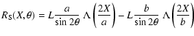
If one calibrates the focal plane in terms of angular units,
![]() and
and
![]() ,
the intensity
,
the intensity
![]() can be written
as:
can be written
as:
We consider for later use several properties of
![]() ,
for the general case in which P(x,y) presents a non-uniform complex transmission.
For this we make use of the two integrated quantities
,
for the general case in which P(x,y) presents a non-uniform complex transmission.
For this we make use of the two integrated quantities
![]() and
and
![]() that play an important role in the efficiency of
a telescope:
0pt
that play an important role in the efficiency of
a telescope:
0pt
The intensity at the center of the diffraction pattern is
given by:
In terms of signal and image processing, the PSF is a function
whose integral equals 1. We obtain such a function, which we
denote
![]() by dividing
by dividing
![]() by
by
![]() .
If we divide
.
If we divide
![]() by
by
![]() we obtain a function that is equal to
1 at the origin and which we denote
we obtain a function that is equal to
1 at the origin and which we denote
![]() .
These
three functions are related to one another by the relation:
.
These
three functions are related to one another by the relation:
Rather than using an angle to determine the resolution of a
telescope, one may use an angular surface ![]() for characterizing the spread of the PSF on the sky. Generalizing the
concept of equivalent width used in Fourier transform theory to
two dimensions, the equivalent angular surface
for characterizing the spread of the PSF on the sky. Generalizing the
concept of equivalent width used in Fourier transform theory to
two dimensions, the equivalent angular surface ![]() (or
equivalent solid angle) may be written as:
(or
equivalent solid angle) may be written as:
For a perfect telescope with a circular aperture, the intensity in
the focal plane can be written as:
The Airy pattern presents relatively strong wings that
hamper the observation of a close-by faint source like an exoplanet. The envelope of the Airy
wings decreases only as the cube of the
distance from the center. Rings of the diffraction pattern remain above 10-3 up to the
![]() ring, and decrease below 10-4 after the
ring, and decrease below 10-4 after the
![]() ring only. The diffraction pattern drops below 10-5 only at a distance
greater than
ring only. The diffraction pattern drops below 10-5 only at a distance
greater than
![]() ,
and would require a distance of
,
and would require a distance of
![]() to reach a value of 10-9, comparable to what is expected for a terrestrial
exoplanet. This effect is strong enough to consider the perturbations
produced by other distant bright stars in the field.
to reach a value of 10-9, comparable to what is expected for a terrestrial
exoplanet. This effect is strong enough to consider the perturbations
produced by other distant bright stars in the field.
A reduction of the strength of the Airy wings is
possible, at the cost of a widening of the central part of the
pattern (and therefore of ![]() ), modifying the pupil in shape
or transmission. The first use of such apertures seems to have
been published by Couder & Jacquinot (1939) who used a
square aperture for the detection of faint spectral lines with a
dynamic range up to 104. They wrote the PSF as the following
product of a function of
), modifying the pupil in shape
or transmission. The first use of such apertures seems to have
been published by Couder & Jacquinot (1939) who used a
square aperture for the detection of faint spectral lines with a
dynamic range up to 104. They wrote the PSF as the following
product of a function of ![]() with a function of
with a function of ![]() of
the form:
of
the form:
Nisenson & Papaliolios (2001), in their project of an Apodized Square Aperture (ASA),
use this same shaped aperture for which the effect of wing reduction is enforced by
an apodization with two separable functions of ![]() and
and ![]() .
As in
the Couder & Jacquinot example, the aperture is
utilized at
.
As in
the Couder & Jacquinot example, the aperture is
utilized at
![]() of the axes.
of the axes.
A unified presentation of diffraction patterns of shaped and
apodized apertures can be presented using the Radon transform.
This can be obtained by expressing the focal plane intensity in
radial coordinates. For that, we make use of well known
properties of two-dimensional Fourier transforms, in particular
the so-called central slice theorem. This theorem allows us to
write the diffraction pattern in the direction ![]() as the
one-dimensional Fourier transform of the Radon transform of the
aperture. This can be demonstrated as follows. The Fourier
transform
as the
one-dimensional Fourier transform of the Radon transform of the
aperture. This can be demonstrated as follows. The Fourier
transform
![]() of the aperture transmission function
P(x,y) can be written as:
of the aperture transmission function
P(x,y) can be written as:
![\begin{figure}
\par {\includegraphics[width=6.7cm,clip]{2311fi01.eps} }
\end{figure}](/articles/aa/full/2005/17/aa2311/img90.gif) |
Figure 1:
Illustration of the computation of the aperture
Radon transform
|
| Open with DEXTER | |
![\begin{figure}
\par {\includegraphics[width=6.1cm,clip]{2311fi02.eps} }
\end{figure}](/articles/aa/full/2005/17/aa2311/img92.gif) |
Figure 2:
Radon transform
|
| Open with DEXTER | |
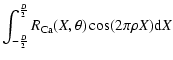
An illustration of the computation of the Radon transform
![]() is given in Fig. 1. It corresponds, for given X and
is given in Fig. 1. It corresponds, for given X and ![]() to the integral of the aperture
transmission function along a line (segment AB in
Fig. 1) perpendicular to the direction of
diffraction. The result that would be obtained for a clear
elliptic aperture is drawn in Fig. 2. In medical
tomography, this integral is called a projection; in this domain,
the interest is in the inversion of the Radon transform to
retrieve P(x, y) knowing
to the integral of the aperture
transmission function along a line (segment AB in
Fig. 1) perpendicular to the direction of
diffraction. The result that would be obtained for a clear
elliptic aperture is drawn in Fig. 2. In medical
tomography, this integral is called a projection; in this domain,
the interest is in the inversion of the Radon transform to
retrieve P(x, y) knowing
![]() .
This is mainly done
numerically, using filtered back-projection. It might
be of interest for astronomy if we seek to find the aperture that produces a
given PSF, but this delicate inverse problem (which does not
necessarily have a solution) will not be treated here.
.
This is mainly done
numerically, using filtered back-projection. It might
be of interest for astronomy if we seek to find the aperture that produces a
given PSF, but this delicate inverse problem (which does not
necessarily have a solution) will not be treated here.
Let us illustrate the Radon approach for the examples of a circular aperture, a square aperture and a Gaussian shaped aperture.
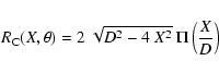
A clear circular
aperture can be taken as the basis for an un-shaped, un-apodized
aperture. Its Radon transform is independent of ![]() ,
and
simply equal to the cord of the circle:
,
and
simply equal to the cord of the circle:
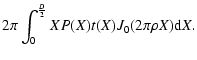
The one-dimensional Fourier transform of
![]() gives
the amplitude of the Airy function (Eq. (10)). If we
apply to this aperture a circular-symmetric apodization function
t(r), its Radon transform
gives
the amplitude of the Airy function (Eq. (10)). If we
apply to this aperture a circular-symmetric apodization function
t(r), its Radon transform
![]() will be an even
function of X, independent of
will be an even
function of X, independent of ![]() .
The circular diffraction
pattern can be computed using either Eq. (13) or by
the Hankel transform of P(r) t(r):
.
The circular diffraction
pattern can be computed using either Eq. (13) or by
the Hankel transform of P(r) t(r):
The treatment of an elliptical aperture (our example in
Fig. 1) could be done as a generalization of that of
a circular aperture. The circular symmetry is obviously lost, but
the value of
![]() ,
given in the caption of
Fig. 2, resembles that obtained for a circle; most
of the above results remain valid after a geometrical
transformation that consists of a similitude in the direction of
one of the axes of the ellipse.
,
given in the caption of
Fig. 2, resembles that obtained for a circle; most
of the above results remain valid after a geometrical
transformation that consists of a similitude in the direction of
one of the axes of the ellipse.
![\begin{figure}
\par {\includegraphics[width=7.7cm,clip]{2311fi03.eps} }
\end{figure}](/articles/aa/full/2005/17/aa2311/img108.gif) |
Figure 3:
Illustration of the Radon approach for a square aperture.
Top left: gray level representation of the Radon transform
|
| Open with DEXTER | |
A square aperture can be considered
as the simplest shaped aperture. Its throughput compared with the
circular aperture is less by ![]() (square inscribed in the
circular aperture). After a few computations, the formula below
can be derived to give the Radon transform of a square:
0pt
(square inscribed in the
circular aperture). After a few computations, the formula below
can be derived to give the Radon transform of a square:
0pt
Various kinds of apodization can be used together with a
rectangular aperture. Nisenson and Papaliolios for ASA proposed
to use Sonine apodizations, of the form
![]() .
These apodizations were compared to
prolate spheroidal apodizations by Soummer et al. (2002),
who also give expressions for various apodizations and
corresponding PSFs.
.
These apodizations were compared to
prolate spheroidal apodizations by Soummer et al. (2002),
who also give expressions for various apodizations and
corresponding PSFs.
A shaped aperture can be constructed using simple or very complex
contours. The elliptic aperture given as an example in
Fig. 1 is a simple modification of the circular
aperture, as already discussed. To the contrary, the aperture
proposed by Kasdin et al. (2003) uses masks with 6 to
8 elongated transparent zones. In such a case, it is difficult
to find an analytical expression for the Radon transform, and the
computation must be made numerically. This is already the case for
the aperture drawn in Fig. 4
whose contour is defined by two truncated
Gaussian curves of the form
![]() .
The resulting
figure is not convex; for some values of
.
The resulting
figure is not convex; for some values of ![]() and X, the
integration line (a line such as AB in Fig. 1)
crosses the aperture in 4 points. The corresponding value for
and X, the
integration line (a line such as AB in Fig. 1)
crosses the aperture in 4 points. The corresponding value for
![]() is double peaked, and gives strong diffraction arms
outside the region where
is double peaked, and gives strong diffraction arms
outside the region where ![]() is close to 0.
is close to 0.
| |
Figure 4:
Left: shaped aperture (Gaussian contour) with its
corresponding diffraction pattern inside, in a
representation similar to that of Jacquinot (1950).
Middle: Radon transform
|
| Open with DEXTER | |
As already indicated, several recent studies have been made on
various shaped apertures (Kasdin et al. 2003; Vanderbei
et al. 2003b,a). These authors emphasize
two advantages of shaped apertures compared to apodized ones. The
first is the simplicity of fabrication, which is obvious. The
second is that, for a similar result, shaped apertures provide a
better intensity throughput than apodized apertures, because the
term
|P(x,y)|2 makes the intensity flux
![]() to be
smaller than
to be
smaller than
![]() for an apodized aperture, while
for an apodized aperture, while
![]() for a shaped aperture. With the Radon approach
of Eqs. (13) and (14), it is clear that
different shaped or apodized
apertures can lead to the same value of
for a shaped aperture. With the Radon approach
of Eqs. (13) and (14), it is clear that
different shaped or apodized
apertures can lead to the same value of
![]() for a given direction
for a given direction ![]() .
But different apertures cannot
give the same
.
But different apertures cannot
give the same
![]() for all
for all ![]() values, unless they
are identical. This derives from the inverse properties of both
Fourier and Radon transforms. A shaped aperture cannot wholly
replace an apodized aperture and vice versa.
values, unless they
are identical. This derives from the inverse properties of both
Fourier and Radon transforms. A shaped aperture cannot wholly
replace an apodized aperture and vice versa.
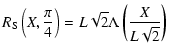
An illustration of this is made in Fig. 5, which
compares the diffraction patterns of two apertures included in a
rectangle of surface S. One aperture is apodized by a linear
function in one direction (of the form 1-2|x|/L, L being the
length of the rectangle); the other aperture is shaped in the
form of a rhombus. Both apertures give the same triangle function
for R(X,0). The value I(0,0) of the diffraction pattern at the
center is the same for these two apertures and equals 1/4 (times
the constant factor
![]() ). The throughput
favors the shaped aperture, as claimed by the authors using these
techniques: it is of 1/2 for the shaped aperture (shaping
reduces the aperture area by a factor 2), against only 1/3 for
the apodized aperture (result of the integration of
(1-2|x|/L)2). But this apparent gain is misleading, and
expresses only the fact that the intensity is uselessly spread in
the other directions by the shaped aperture. This is clearly
visible in Fig. 5, where the diffraction takes the
shape of an X elongated in the vertical direction, preventing any
useful planet detection in this region. The apodized aperture is
much more efficient for the whole plane on average. It makes it
possible to discover an exoplanet in a wider region. This can be
quantified using the Strehl factor
). The throughput
favors the shaped aperture, as claimed by the authors using these
techniques: it is of 1/2 for the shaped aperture (shaping
reduces the aperture area by a factor 2), against only 1/3 for
the apodized aperture (result of the integration of
(1-2|x|/L)2). But this apparent gain is misleading, and
expresses only the fact that the intensity is uselessly spread in
the other directions by the shaped aperture. This is clearly
visible in Fig. 5, where the diffraction takes the
shape of an X elongated in the vertical direction, preventing any
useful planet detection in this region. The apodized aperture is
much more efficient for the whole plane on average. It makes it
possible to discover an exoplanet in a wider region. This can be
quantified using the Strehl factor ![]() that strongly favors
the apodized aperture for which
that strongly favors
the apodized aperture for which
![]() against only 1/2for the shaped aperture.
against only 1/2for the shaped aperture.
Similar conclusions can be drawn for the other shaped apertures recently
proposed in the literature. In fact, to give better useful throughput
than an apodized aperture and the same diffraction pattern in a given direction
![]() a shaped aperture should be able to produce a value
a shaped aperture should be able to produce a value
![]() ,
with k greater than 1. This is not possible since the maximal value cannot exceed
the length of the aperture in the transverse direction. The
interest of a shaped aperture that remains is its ease of fabrication.
,
with k greater than 1. This is not possible since the maximal value cannot exceed
the length of the aperture in the transverse direction. The
interest of a shaped aperture that remains is its ease of fabrication.
![\begin{figure}
\par {\includegraphics[width=8.1cm,clip]{2311fi05.eps} }
\end{figure}](/articles/aa/full/2005/17/aa2311/img123.gif) |
Figure 5:
Top: two aperture transmissions included in a rectangle and
giving exactly the same triangle function for
|
| Open with DEXTER | |
Now let us consider the more general case of apodization. If we
seek to have a point spread function with reduced side-lobes in a
given direction ![]() ,
then we want a smooth value for
,
then we want a smooth value for
![]() in that direction. Since the work of Duffieux
(1946), it is known that the diffracted amplitude in
the far wings decreases as a power series of the form
f(n-1)
x-n, where f(n) is the value of the
in that direction. Since the work of Duffieux
(1946), it is known that the diffracted amplitude in
the far wings decreases as a power series of the form
f(n-1)
x-n, where f(n) is the value of the ![]() derivative
of the transmission at the edge of the aperture (for a full
aperture with no central obscuration). This result is derived from
repeated integration by parts of the diffraction integral written
as a Fourier transform. The same result applies for the Fourier
transform of
derivative
of the transmission at the edge of the aperture (for a full
aperture with no central obscuration). This result is derived from
repeated integration by parts of the diffraction integral written
as a Fourier transform. The same result applies for the Fourier
transform of
![]() .
A square aperture gives a decreasing
amplitude in 1/x along the axes because the Radon transform
.
A square aperture gives a decreasing
amplitude in 1/x along the axes because the Radon transform
![]() is not zero at X=L/2 (Eq. (11)). With
this idea in mind, one would propose apodizing functions equal to
zero at the edge of the aperture with the first non-zero
derivative as high as possible. Jacquinot & Roizen-Dossier
(1964) pointed out that this goal is difficult to
realize in practice, because the optical density of an absorbing
medium cannot rise from 0 to infinity from the center to the
edge of the aperture. As a consequence, the transmission at the
margin of the aperture may be very low, but not zero. However, the
overall shape of the aperture may compensate that effect. Indeed,
because of the integration in Eq. (9), a strictly
convex two-dimensional aperture (boundary containing no line
segment) gives a value of zero for
is not zero at X=L/2 (Eq. (11)). With
this idea in mind, one would propose apodizing functions equal to
zero at the edge of the aperture with the first non-zero
derivative as high as possible. Jacquinot & Roizen-Dossier
(1964) pointed out that this goal is difficult to
realize in practice, because the optical density of an absorbing
medium cannot rise from 0 to infinity from the center to the
edge of the aperture. As a consequence, the transmission at the
margin of the aperture may be very low, but not zero. However, the
overall shape of the aperture may compensate that effect. Indeed,
because of the integration in Eq. (9), a strictly
convex two-dimensional aperture (boundary containing no line
segment) gives a value of zero for
![]() at the edge for
any
at the edge for
any ![]() value.
value.
| |
Figure 6:
Example of projections
|
| Open with DEXTER | |
Several apertures recently proposed, such as the checkerboard
aperture of Vanderbei et al. (2004), do not obey that
requirement and present discontinuities because they are made of
disjoint transmission regions. These discontinuities induce
step-like variations in
![]() that produce ghosts toward
some directions, or diffracted amplitudes for circular concentric
rings (Vanderbei et al. 2003a,b). In the
latter case,
that produce ghosts toward
some directions, or diffracted amplitudes for circular concentric
rings (Vanderbei et al. 2003a,b). In the
latter case,
![]() can be written as a weighted sum of
functions of the form given in Eq. (15). An elementary
representation of such an aperture is the classical circular
aperture with central obstruction that can be written as
can be written as a weighted sum of
functions of the form given in Eq. (15). An elementary
representation of such an aperture is the classical circular
aperture with central obstruction that can be written as
![]() ,
where D and d are the outer and
inner diameters of the aperture. This function is continuous, but
not its derivative at the points |X|=d/2, as it can be seen for
the dashed curves of Fig. 6. To reduce the side
lobes, Jacquinot & Roizen-Dossier (1964) proposed to
use pupil transmissions that decrease both toward the edge
and toward the center of the aperture; for that kind of
apodization they used
a function of the form J2(r). In
Fig. 6 we have drawn for comparison the results on
the projections for the two cases of apodization (we used a
simple polynomial function in this example). The projection
corresponding to a double apodization presents a smooth
structure, while that corresponding only to a single apodization
presents a structure with unwanted peaks.
,
where D and d are the outer and
inner diameters of the aperture. This function is continuous, but
not its derivative at the points |X|=d/2, as it can be seen for
the dashed curves of Fig. 6. To reduce the side
lobes, Jacquinot & Roizen-Dossier (1964) proposed to
use pupil transmissions that decrease both toward the edge
and toward the center of the aperture; for that kind of
apodization they used
a function of the form J2(r). In
Fig. 6 we have drawn for comparison the results on
the projections for the two cases of apodization (we used a
simple polynomial function in this example). The projection
corresponding to a double apodization presents a smooth
structure, while that corresponding only to a single apodization
presents a structure with unwanted peaks.
![\begin{figure}
\par {\includegraphics[width=5.1cm,clip]{2311fi07.eps} }
\end{figure}](/articles/aa/full/2005/17/aa2311/img127.gif) |
Figure 7:
Principle of a spiral aperture whose projections
|
| Open with DEXTER | |
A difficulty that remains is the practical implementation of these continuous apodizations. Good results seem to have been obtained in the past by Jacquinot who used a special apparatus. Recent developments have been made that use interferometric apodizations, as proposed by Aime et al. (2001) and Martinache (2003). The reader will find several other techniques in the selection of papers by Mills & Thompson (2003) already quoted. Some of the techniques proposed are very surprising, such as the apodization using frustrated total reflection proposed by Diels (1975). Nevertheless, it might be interesting to use discrete pupil masks because they appear to be easy to realize from an engineering point of view. In that case we may try to overcome the problem of discontinuities. As a line of investigation one might imagine a discrete aperture drawn continuously in the plane. An example of that is the one in the form of a spiral drawn with a pencil of variable width in Fig. 7. Note that this figure is given only for illustration, and no theory was developed for it by the author. More complex Hilbert plane-filling curves might also be used for the same purpose. We do not intend to develop their study here, and come back to apertures with variable transmission.
For an even pattern,
![]() must be even. In that case, the
modulus squared of the real and imaginary parts of the transform
add independently, and there is no advantage for
must be even. In that case, the
modulus squared of the real and imaginary parts of the transform
add independently, and there is no advantage for
![]() not to be real. This result was already obtained by
Dossier et al. (1954) using a different reasoning. It might in
principle present negative parts corresponding to phase
not to be real. This result was already obtained by
Dossier et al. (1954) using a different reasoning. It might in
principle present negative parts corresponding to phase ![]() ,
but this is unlikely to be realized because of the difficulty of
obtaining achromatic phase shifters. We therefore come to the
conclusion that the apodizing function should have a real
transmission between 0 and 1. It should be noted moreover that all
of the classical apodizing functions proposed in the literature of
signal processing (Bartlett, Blackman, Cosine, Gaussian, Hamming,
Hanning, Welch or others) described for example in Harris
(1978) are positive-only functions.
,
but this is unlikely to be realized because of the difficulty of
obtaining achromatic phase shifters. We therefore come to the
conclusion that the apodizing function should have a real
transmission between 0 and 1. It should be noted moreover that all
of the classical apodizing functions proposed in the literature of
signal processing (Bartlett, Blackman, Cosine, Gaussian, Hamming,
Hanning, Welch or others) described for example in Harris
(1978) are positive-only functions.
Jacquinot & Roizen-Dossier (1964) consider several techniques for a systematic search for pupil functions with given apodizing properties, such as to have a dark region in the diffraction pattern, an idea further envisaged by Malbet et al. (1995), or to consider several criteria, among them the rate of decrease of energy already discussed, the spreading factor, or the maximum encircled energy. For the latter case, they failed to describe the prolate spheroidal functions that were discovered at that time by Slepian (1964) and Slepian & Pollak (1961) and whose application to optics was later reviewed by Frieden (1971).
![\begin{figure}
\par {\includegraphics[width=6.5cm,clip]{2311fi08.eps} } \end{figure}](/articles/aa/full/2005/17/aa2311/img129.gif) |
Figure 8:
Examples of prolate
apodization functions for a circular aperture. Top: radial cuts of the transmission in amplitude, for a
telescope of diameter 1 (radius 0.5). Bottom: corresponding PSFs, normalized to 1 at the origin
(
|
| Open with DEXTER | |
| |
Figure 9:
Representation on a semi-logarithmic
scale of (1) the aperture equivalent resolving solid angle |
| Open with DEXTER | |
An example of prolate spheroidal function and corresponding PSF is
given in Fig. 8. For it, we used a special program
written by P.E. Falloon (Falloon et al. 2003) in
Mathematica (Wolfram 1999) to compute prolate
circular spheroidal functions. The behavior of prolate apodization
is quite different to the other apodizations. Indeed, the rate of
attenuation of the wings remains r-3 as for the
Airy pattern, but starts at a much lower level. This is not surprising
because prolate apodizations do not end with zero at the edge of the aperture,
and we refer the reader to the reasoning conducted above on the behavior of apodizations
and strictly convex apertures.
For a circular prolate spheroidal function,
the values of
![]() ,
,
![]() and
and ![]() are represented in
Fig. 9 as a function of the parameter c that
defines the strength of the apodization (see for example Frieden
(1971) for description of this parameter). In the same
graph, we have plotted the decrease of the level of the wings
compared to that of the Airy function. For some aspects, the
prolate functions may be considered as the best apodizers (they
maximize the encircled energy). However, their importance for
apodization is not so fundamental as in coronagraphy (Soummer et al. 2002).
are represented in
Fig. 9 as a function of the parameter c that
defines the strength of the apodization (see for example Frieden
(1971) for description of this parameter). In the same
graph, we have plotted the decrease of the level of the wings
compared to that of the Airy function. For some aspects, the
prolate functions may be considered as the best apodizers (they
maximize the encircled energy). However, their importance for
apodization is not so fundamental as in coronagraphy (Soummer et al. 2002).
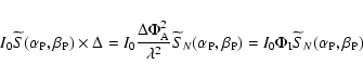
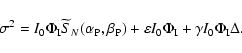
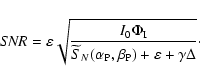
The detection of a signal embedded in noise is a classical problem of signal detection theory (Michel & Ferrari 2003). For large difference between the planet and the background and a large number of collected photons a classical signal-to-noise analysis can be utilized.
The intensity produced in the focal plane by the star is
![]() ,
as described by Eq. (2).
The constant term I0 depends on the brightness of the star,
and must be expressed in number of photons. If
,
as described by Eq. (2).
The constant term I0 depends on the brightness of the star,
and must be expressed in number of photons. If
![]() is
the intensity ratio between the planet and the star, the function
corresponding to a planet at the position
is
the intensity ratio between the planet and the star, the function
corresponding to a planet at the position
![]() is
is
![]() .
To obtain a simple
expression for the SNR of the experiment, we make two simplifying
assumptions. We assume that the residual diffraction wings of the
star can be approximated as a local constant background of value
.
To obtain a simple
expression for the SNR of the experiment, we make two simplifying
assumptions. We assume that the residual diffraction wings of the
star can be approximated as a local constant background of value
![]() ,
where
,
where
![]() corresponds to a local mean
of
corresponds to a local mean
of
![]() ,
integrated over a region of size
,
integrated over a region of size
![]() .
Moreover, we make the optimistic assumption that all
the light of the planet can be collected in a pixel, or a group of
pixels, of angular equivalent surface
.
Moreover, we make the optimistic assumption that all
the light of the planet can be collected in a pixel, or a group of
pixels, of angular equivalent surface ![]() .
For simplicity of
notations, the overall efficiency of the optical system and
detector is assumed to be 1; if not, this would change only the
value of I0.
.
For simplicity of
notations, the overall efficiency of the optical system and
detector is assumed to be 1; if not, this would change only the
value of I0.
![\begin{figure}
\par {\includegraphics[width=6cm,clip]{2311fi10.eps} } \end{figure}](/articles/aa/full/2005/17/aa2311/img137.gif) |
Figure 10:
Schematic representation of a planet over a strong
background due for example to the wings of the diffraction pattern of
the star. We assume in this model that all the photons
from the planet gather in a surface |
| Open with DEXTER | |
| |
Figure 11:
Representation of the logarithm of the SNR as a function of
the strength of apodization (parameter c) for a prolate apodized circular telescope, as given by
Eq. (20),
for the case of a background free observation
( |
| Open with DEXTER | |
| |
Figure 12:
Similar to Fig. 11,
for a fixed value
|
| Open with DEXTER | |
With this model the expected number of photons collected for the
planet is (optimistically) estimated to be
![]() .
Within the resolution surface
.
Within the resolution surface ![]() ,
the
number of photons due to the diffraction of the star is given by
the volume of the cylinder below the planet as schematized in
Fig. 10:
,
the
number of photons due to the diffraction of the star is given by
the volume of the cylinder below the planet as schematized in
Fig. 10:
A strong apodization is more effective than a weak one, and permits
considerable improvement of the SNR. For low c values (up to 4or so), the apodization is not efficient since
![]() decreases as fast as the wings. For very large values of c, the
SNR decreases when the number of photons in the wings under the
planet is comparable to that in the planet, leading to an optimal
c value. For a small dynamical range between the sources,
apodization is not efficient. This is the case for example for
decreases as fast as the wings. For very large values of c, the
SNR decreases when the number of photons in the wings under the
planet is comparable to that in the planet, leading to an optimal
c value. For a small dynamical range between the sources,
apodization is not efficient. This is the case for example for
![]() (double star of 5 mag difference),
at least for the separation chosen (
(double star of 5 mag difference),
at least for the separation chosen (
![]() )
in
Fig. 11. From this example we may conclude that in
general the larger the magnitude difference between the star and
the planet, the stronger the apodization to
use.
)
in
Fig. 11. From this example we may conclude that in
general the larger the magnitude difference between the star and
the planet, the stronger the apodization to
use.
The effect of the background may reduce the interest of
apodization because it reintroduces the effect of the equivalent
area ![]() .
We show it in an example in Fig. 12,
where we have represented the SNR for
.
We show it in an example in Fig. 12,
where we have represented the SNR for
![]() and
different values of the background coefficient
and
different values of the background coefficient ![]() .
In that
case the SNR is both sensitive to the throughput and to the
equivalent surface of resolution
.
In that
case the SNR is both sensitive to the throughput and to the
equivalent surface of resolution ![]() .
The optimum is obtained
for a lower value of the parameter c; it still corresponds to a
strong apodization. A very strong background (large
.
The optimum is obtained
for a lower value of the parameter c; it still corresponds to a
strong apodization. A very strong background (large ![]() values) makes apodization useless.
values) makes apodization useless.
It is possible to obtain a simplified form for the SNR if we make
the assumption that both
![]() and
and
![]() remain
small compared to the wings of the PSF. In that case,
Eq. (20) reduces to a function
remain
small compared to the wings of the PSF. In that case,
Eq. (20) reduces to a function
![]() that
only depends, for the circular prolate apodization, on the
parameter c and the distance star to planet
that
only depends, for the circular prolate apodization, on the
parameter c and the distance star to planet ![]() (
(![]() here stands
for
here stands
for
![]() ):
):
![\begin{figure}
\par {\includegraphics[width=6.8cm,clip]{2311fi13.eps} }
\end{figure}](/articles/aa/full/2005/17/aa2311/img158.gif) |
Figure 13:
Representation on a logarithmic scale
of the term
|
| Open with DEXTER | |
The assumptions we have used to derive
Eq. (20) are
optimistic (all the flux of the planet within ![]() )
and
cannot be verified in practice. It is possible however to use a
matched filter, convolving the image with the PSF, or an estimate
of the PSF (Aime 2004). This will not change the level
of the background. It will slightly modify the maximum collected
flux for the planet. As described by Aime & Soummer
(2003), a new quantity
)
and
cannot be verified in practice. It is possible however to use a
matched filter, convolving the image with the PSF, or an estimate
of the PSF (Aime 2004). This will not change the level
of the background. It will slightly modify the maximum collected
flux for the planet. As described by Aime & Soummer
(2003), a new quantity
![]() should be substituted
to
should be substituted
to
![]() ,
of the form:
,
of the form:
The results presented in this paper can be divided in two parts, the first being a Radon presentation of aperture diffraction effects, and the second a presentation of SNR for apodized apertures.
We have shown that the use of the Radon transform permits a better understanding of diffraction patterns of shaped and apodized apertures, mainly because it makes it possible to reduce the two-dimensional problem to an ensemble of one-dimensional projections. Not all the possibilities allowed by this new approach have been exploited in this paper. We used it for a comparison between shaped, discrete and apodized apertures. Our conclusion favors the apertures with continuous variable transmission, in contradiction with recent publications on this topic. This assumes, of course, that apertures with perfectly controlled transmission can be realized in practice.
Simplified expressions for the SNR of the detection of an exoplanet have also been given. Illustrations for the optimal case of a circular aperture apodized by a prolate spheroidal function have been drawn. Aside from the fact that these functions are optimal in a particular sense for apodization, they make it possible to modulate the strength of the apodization in a continuous way. Several remarks can be made from this study. One is that the apodization must be very strong to be efficient for faint exoplanet detection. The SNR improvement can then be very large. Moreover, the apodization must be adapted to the star to planet distance. As a simple rule-of-thumb, the optimal apodization is the strongest that permits geometric observation of the planet. This conclusion greatly favors the use of the largest possible telescopes.
Acknowledgements
The author would like to thank Peter Falloon for his Mathematica program, Andrea Ferrari, Henri Lantéri and Olivier Michel for stimulating discussions. Thanks are also due to the referee Wesley Traub for very constructive comments, and in particular for his suggestion to use the étendue in Sect. 2.2.