A&A 434, 725-740 (2005)
DOI: 10.1051/0004-6361:20041079
Interplanetary flux rope ejected from an X-ray bright point
The smallest magnetic cloud source-region ever observed
C. H. Mandrini1
- S. Pohjolainen2
- S. Dasso1,3 - L. M. Green4 - P. Démoulin5
- L. van Driel-Gesztelyi5,6,7 -
C. Copperwheat6
- C. Foley6
1 - Instituto de Astronomía y Física del Espacio, CONICET-UBA,
CC. 67,
suc. 28, 1428 Buenos Aires, Argentina![[*]](/icons/foot_motif.gif)
2 -
Tuorla Observatory/VISPA, University of Turku,
21500 Piikkiö, Finland
3 -
Departamento de Física, Facultad de Ciencias Exactas y
Naturales, UBA, Buenos Aires, Argentina
4 -
The Faulkes Telescope Project, Cardiff University, 5
the Parade,
Cardiff, CF24 3YB, UK
5 -
Observatoire de Paris, LESIA, UMR 8109 (CNRS), 92195
Meudon, France
6 -
Mullard Space Science Laboratory, University College London,
Holmbury St. Mary, Dorking, Surrey RH5 6NT, UK
7 -
Konkoly Observatory, Pf. 67, 1525 Budapest, Hungary
Received 13 April 2004 / Accepted 5 January 2005
Abstract
Using multi-instrument and multi-wavelength observations
(SOHO/MDI and EIT, TRACE and Yohkoh/SXT), as well as computing the coronal
magnetic field of a tiny bipole combined with modelling of Wind in situ data, we provide evidences for the smallest event ever observed which
links a sigmoid eruption to an interplanetary magnetic cloud (MC). The tiny
bipole, which was observed very close to the solar disc centre, had
a factor one hundred less flux than a classical active
region (AR). In the corona it had a sigmoidal structure, observed mainly in
EUV, and we found a very high level of non-potentiality
in the modelled magnetic field, 10 times higher than we
have ever found in any AR. From May 11, 1998, and until its disappearance,
the sigmoid underwent three intense impulsive events.
The largest of these events
had extended EUV dimmings and a cusp. The Wind spacecraft detected 4.5 days
later one of the smallest MC ever identified (about a factor one hundred
times less magnetic flux in the axial component than that of an average MC).
The link between this last
eruption and the interplanetary magnetic cloud is supported by several
pieces of evidence: good timing, same coronal loop and MC orientation,
same magnetic field direction and magnetic helicity sign in the coronal
loops and in the MC. We further quantify this link by estimating the
magnetic flux (measured in the dimming regions and in the MC) and the
magnetic helicity (pre- to post-event change in the solar corona and helicity
content of the MC).
Within the uncertainties, both magnetic fluxes and helicities are in reasonable
agreement, which brings further evidences of their link.
These observations show that the ejections of tiny magnetic flux ropes
are indeed possible and put new constraints on CME models.
Key words: Sun: magnetic fields - Sun: corona
Coronal mass ejections (CMEs) are commonly thought to be phenomena
that involve a large-scale reconfiguration of the solar corona,
accompanied by significant disturbances in the solar wind. However,
there is a small subset of events, the so-called narrow CMEs, which do
not conform to this picture. Narrow CMEs are arbitrarily defined as
events whose apparent width is 150 or less and are usually referred
to as rays, spikes, fans, etc. (Munro & Sime 1985; Howard et al. 1985). Within
this category there seems to be two types of ejections: the ones that
exhibit no interior structure and have jet-like characteristics, and
those that are structured and do not show any obvious difference with
large CMEs (Gilbert et al. 2001; Dobrzycka et al. 2003; Harrison et al. 2001). Coronal jets
and CMEs are entirely different phenomena. Jets are thought to be the
result of reconnection between open and closed field lines where the
plasma can be strongly heated and accelerated (Shibata et al. 1992).
CMEs, on the other hand, are often attributed to the release of
magnetic stress stored in a twisted flux tube or in a sheared arcade,
and they involve the ejection of part of the magnetic flux and twist
of the source region into the interplanetary space
(see e.g. Mikic & Linker 1994; Gibson & Low
1998; Antiochos et al.
1999; Lin & Forbes 2000).
Strongly non-potential bipolar magnetic configurations usually have
coronal loops that have a sigmoidal shape when viewed from above.
Sigmoids are preferentially observed in soft
X-rays (Sterling & Hudson 1997). However, in some cases, sigmoids do
appear in EUV images (see e.g. Sterling et al. 2000). Rust & Kumar (1996)
found that many large transient brightenings in X-rays associated with
CMEs were S-shaped. Though the sigmoid - CME connection is still
statistically ambiguous (Glover et al. 2000; Canfield et al. 1999), it has been
suggested that the magnetic helicity content in S-shaped magnetic
configurations may reach a threshold leading to instability and
eruption (van Driel-Gesztelyi et al. 2000;
Török & Kliem 2003 and references therein). In
the same way as CMEs can go from large-scale to very narrow events,
the scale of sigmoidal structures can range from interconnecting
loop size to the size of a typical AR (e.g. Siarkowski et al. 2002).
CMEs appear in the interplanetary medium as interplanetary CMEs (ICMEs).
A subset of these ICMEs, called magnetic clouds (MCs), has
well defined characteristics: a coherent rotation of the magnetic
field vector, an enhanced field strength, as well as, a proton
temperature lower than in the surrounding solar wind
(Burlaga et al. 1981). This subset has been thoroughly studied. There is
increasing evidence that the helicity sign of MCs matches that of
their solar source region (Marubashi 1997; Yurchyshyn et al. 2001; Rust 1994; Bothmer & Schwenn 1994).
Most of the MC studies have so far focused on large scale events which
are observed during a few days (see e.g. Zhao et al. 2001; Lepping et al. 1990), but
recently much smaller interplanetary flux ropes have also been
detected (Shimazu & Marubashi 2000). The statistical distributions of the MC main
physical characteristics, such as their spatial extension, magnetic flux
and helicity, are presently poorly known.
Recognizing the broad spatial and temporal scales in CME source regions,
CMEs and ICMEs, we can ask the following questions:
- 1.
- What is the smallest magnetic bipole that can produce a CME
and launch a twisted flux tube into the interplanetary space?
- 2.
- What is the smallest magnetic flux tube ejected in a
CME that can reach the Earth and still be recognizable as a MC?
![\begin{figure}
\par\includegraphics[width=8.5cm,clip]{1079fi1t.eps}\par\vspace*{...
...m}\includegraphics[width=6.8cm,clip]{1079fi1b.eps}\hspace*{1cm}}
\end{figure}](/articles/aa/full/2005/17/aa1079/Timg16.gif) |
Figure 1:
SXT full disc image at the time of maximum extension of the
sigmoidal X-ray bright point ( top) and the closest in time MDI
magnetogram ( bottom). The bright point is associated to a very small
AR located at disc centre (both shown within the tiny boxes), which
is very far from other ARs. |
| Open with DEXTER |
During a survey of X-ray bright points that showed enhanced emission
at cm- and mm-wavelengths (Pohjolainen 2000), we observed
an isolated radio bright point near the center of the disc on May 11,
1998. We found multi-wavelength evidence of its
eruptive nature, such as elongated sigmoidal loops which later
disappeared, EUV dimmings and cusp formation (in the largest event).
Later, the ejected plasma and magnetic field were
observed in the interplanetary space as a
small MC. The bright point location is shown in soft X-rays just before its
largest eruption, together with a full disc magnetogram,
in Fig. 1. It was well isolated from ARs
present on the Sun. It was also located almost at the disc centre in an
ideal position for any ejecta to reach the Earth.
We first describe, in Sect. 2, the global
evolution of the small bipolar AR at the photospheric level
(magnetic field) and in the corona (EUV and X-rays) from its birth to
its complete decay. Then, the coronal eruptions are analyzed in
Sect. 3. We describe the evidence for the
ejections and quantify the amount of magnetic flux and helicity
involved. We concentrate in the study of the largest event
(in terms of time integrated X-ray flux and EUV dimming extension).
In Sect. 4, we analyze the
interplanetary data plausibly associated with this coronal ejection.
In particular, we derive the same physical quantities as on
the Sun. In Sect. 5, we link the
events observed in the corona and the interplanetary space. Finally,
in Sect. 6, we
conclude that the ejection
differs only in scale from other CME events, being
the same true for its associated MC. We briefly
discuss our results in the context of CME models.
We follow the evolution of the photospheric magnetic field using the
data from the Michelson Doppler Imager (MDI, Scherrer et al. 1995) on
board the Solar and Heliospheric Observatory (SOHO). The magnetograms
are computed from the data taken in five narrowband (94 mÅ)
filtergrams at different positions along the Ni I 6767.8 Å absorption line, formed in the mid-photosphere. The pixel size
of the full disc magnetograms is 1.98 arcsec. MDI returns the
longitudinal magnetic flux density averaged over the pixel field of
view, and from this the flux within a required area can be computed.
To measure the magnetic flux, a polygonal contour, defined by eye,
is fitted around the bipole and the flux is summed within it. In this
way we minimize the contribution of the background field and of the
noise in low field regions ( G). Measurements in the surrounding
quiet Sun regions of the same size give a flux below 3%
of the bipole maximum flux. We correct
all the magnetic field measurements following the results
of Berger & Lites (2003), who analyzed co-temporal and co-spatial MDI and
Advanced Stokes Polarimeter (ASP) data. All the MDI measurements are
below 1200 G, so the relationship between the two instruments is
linear, and we simply multiply the magnetic field measurements by a
factor 1.45 (since Berger & Lites (2003) have found
G). Measurements in the surrounding
quiet Sun regions of the same size give a flux below 3%
of the bipole maximum flux. We correct
all the magnetic field measurements following the results
of Berger & Lites (2003), who analyzed co-temporal and co-spatial MDI and
Advanced Stokes Polarimeter (ASP) data. All the MDI measurements are
below 1200 G, so the relationship between the two instruments is
linear, and we simply multiply the magnetic field measurements by a
factor 1.45 (since Berger & Lites (2003) have found
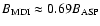 ). According to our measurements, the magnetic flux
of the bipole at peak evolution (average between positive and absolute
value of the negative fluxes, corrected for the flux underestimation
by MDI) was
). According to our measurements, the magnetic flux
of the bipole at peak evolution (average between positive and absolute
value of the negative fluxes, corrected for the flux underestimation
by MDI) was
 Mx. This peak flux puts this bipole
into the "small active region'' category that are defined to be in a
flux range of
Mx. This peak flux puts this bipole
into the "small active region'' category that are defined to be in a
flux range of
 Mx
(Schrijver & Zwaan 2000). These small ARs are frequently spotless or at
most contain pores. In the MDI white-light images this bipole
appeared spotless and even poreless during its entire existence.
Mx
(Schrijver & Zwaan 2000). These small ARs are frequently spotless or at
most contain pores. In the MDI white-light images this bipole
appeared spotless and even poreless during its entire existence.
The lifetime of ARs is roughly proportional to their flux content at
maximum development. Flux decay rate is between
 Mx/day (Golub 1980; Harvey 1993, respectively). For an AR
having a magnetic flux of
Mx at peak evolution,
the entire lifetime from birth to disappearance is short since the bipole
is expected to exist for about 1.5 - 3 days. In this particular
case, we indeed observed the bipole for 64 h (2.7 days, see
Fig. 2).
Mx/day (Golub 1980; Harvey 1993, respectively). For an AR
having a magnetic flux of
Mx at peak evolution,
the entire lifetime from birth to disappearance is short since the bipole
is expected to exist for about 1.5 - 3 days. In this particular
case, we indeed observed the bipole for 64 h (2.7 days, see
Fig. 2).
![\begin{figure}
\par\hspace*{2mm}\includegraphics[width=7.6cm,clip]{1079fi2t.eps}\par\vspace*{3mm}
\includegraphics[width=7.9cm,clip]{1079fi2b.eps}
\end{figure}](/articles/aa/full/2005/17/aa1079/Timg22.gif) |
Figure 2:
Magnetic ( top) and X-ray flux evolution ( bottom) from
the emergence to the disappearance of the small active region.
The positive (negative) magnetic flux is shown with continuous
(dashed) line.
There are three main bursts in X-rays (marked with arrows in the bottom
figure), which all occurred on May 11: the first at  01:00 UT,
the second
at 07:00 UT, and the third
at 09:00 UT. 01:00 UT,
the second
at 07:00 UT, and the third
at 09:00 UT. |
| Open with DEXTER |
We analyze the evolution of the X-ray flux of this small spotless
AR with the Yohkoh/Soft X-ray Telescope (SXT, Tsuneta et al. 1991).
The full-disc images have a pixel size of 5 arcsec. We used the software
SXT_FLUX with a fixed temperature of 2 MK for this AR, which we obtained from
the temperature
analysis using the thin aluminum (Al1) and the Dagwood filters (Al-Mg).
Outside flaring times (i.e. outside X-ray peaks), the X-ray flux
is correlated in time with the total magnetic flux
(Fig. 2). This is in agreement with several
previous studies. Harvey (1997) showed that the total magnetic
flux and the intensity increase of an X-ray bright point, related to
an emerging bipole, were almost linearly
proportional. Fisher et al. (1998) found that the X-ray luminosity
( )
of solar ARs is best correlated with the total unsigned
magnetic flux (
)
of solar ARs is best correlated with the total unsigned
magnetic flux (
 )
of the region. The
)
of the region. The
 relationship was found to follow a power-law with an exponent of 1.19.
Pevtsov et al. (2003) extended this result to a broad range of structures on the
Sun (quiet Sun, X-ray bright points, active regions, and
integrated solar disc) and to active stars (dwarf and pre-main-sequence).
relationship was found to follow a power-law with an exponent of 1.19.
Pevtsov et al. (2003) extended this result to a broad range of structures on the
Sun (quiet Sun, X-ray bright points, active regions, and
integrated solar disc) and to active stars (dwarf and pre-main-sequence).
However, there appear to be differences between the shapes of the magnetic
and X-ray flux evolution curves. Magnetic flux peaks about eleven hours
after the start of emergence, then decreases steadily. The X-ray flux, outside
flaring times, reaches maximum ten hours later than the magnetic
flux, which may be regarded as the storage time of the free magnetic energy.
The soft X-ray light curve presents several peaks
(Fig. 2). The first small flare event is
observed as early as about two hours after the appearance of the XBP,
and about eight hours after the start of the emergence of the bipole
on 10 May. The most intense events are observed during May 11
(Fig. 2). The exact times of the X-ray bursts are
difficult to define because of the low temporal cadence of SXT
full-disc images.
The first event started between the images taken at
00:42 UT and 00:51 UT. At 01:08 UT, the SXT flux had gone down to the
pre-event level, so its maximum duration was 26 min. This first
X-ray burst was also observed by the Nobeyama Radioheliograph
(Nishio et al. 1994)
at 17 GHz (1 s time cadence). From the constructed radio flux
curve, the burst began at 00:45 UT, peaked at 00:48 UT and ended at
00:58 UT, having a total duration of 13 min.
Two close in time X-ray bursts followed the first one.
The second event occurred between 06:00 UT and 08:00 UT, while the third
one started between SXT full-disc images at 08:03 UT and 08:44 UT and had a
maximum between 08:03 UT and 09:16 UT. The post-maximum evolution of this
event was imaged with a higher temporal cadence and we can define its end as
11:00 UT. Then, its duration was of about 3 h. Unfortunately, this
third burst occurred too late for Nobeyama and was not imaged in radio.
The orientation of the magnetic bipole was observed to change
with time (Fig. 3), the axis joining both polarities
rotated. Such rotation could come from the emergence of a non-planar
magnetic flux tube (as studied for ARs, López Fuentes et al. 2003). However,
in the present case most of the rotation is likely to be apparent and
probably due to the emergence of a strongly twisted flux tube, as
discussed below.
The presence of twist in an emerging flux tube can influence the
distribution of the line-of-sight magnetic field in such a way that,
for a negative twist, the preceding polarity extends along the
northern boundary of the following polarity (forming an elongated
"magnetic tongue''). This has been proposed by
López Fuentes et al. (2000, see their Fig. 5 and corresponding text).
In the two first magnetograms of Fig. 3, only
the upper part of the flux
tube (i.e. above the flux tube axis) has emerged across the photosphere.
At this time, mostly the
azimuthal component (associated to the twist) is contributing to the
longitudinal field (which mainly corresponds to the vertical component
because of the near central disc position).
As the emergence proceeds, the axial magnetic component of the flux tube
contributes more to the vertical photospheric component, forming the
classical separating polarities in magnetic bipoles (see magnetograms at
12:47 and
19:11 UT in Fig. 3). At these times, the photospheric
magnetic distribution is formed by two separating polarities and by
two magnetic tongues. As emergence continues, the magnetic tongues
retract (see magnetograms from 1:39 UT to 12:51 UT on May 11) because (i) the
azimuthal component is less important closer to the central part of
the flux tube and (ii) it has a smaller vertical projection in the legs of the
flux tube.
In the case of a strongly twisted flux tube, this evolution leads to an
apparent rotation of the photospheric magnetic polarities by about 90 degrees. The orientation (or chirality) of the magnetic tongues is directly
linked to the sign of the twist (López Fuentes et al. 2000). Therefore, we conclude from
the evolution of the longitudinal field distribution that the emerging flux
tube had a strong negative twist.
The complete evolution of the EUV emission of this small AR is best
covered by the observations obtained with the SOHO/Extreme-Ultraviolet
Imaging Telescope (EIT, Delaboudiniere et al. 1995). EIT observes the full
Sun regularly with four different filters and with a pixel size of 2.6 arcsec
(Fig. 4). Globally
the EUV emission followed the evolution of the photospheric magnetic field
(Fig. 3); in particular, the emission extends and rotates in
parallel to the photospheric "boundary conditions''.
![\begin{figure}
\par\includegraphics[width=7.5cm,height=18cm,clip]{1079fi3.eps}
\end{figure}](/articles/aa/full/2005/17/aa1079/Timg26.gif) |
Figure 3:
Photospheric magnetograms from SOHO/MDI showing the
full evolution of the bright point region from May 10 to 12, 1998.
The field of view is
 arcsec
(1.98 arcsec per pixel), the
maps have been coaligned and derotated to central meridian position
(11 May 04:15 UT). arcsec
(1.98 arcsec per pixel), the
maps have been coaligned and derotated to central meridian position
(11 May 04:15 UT). |
| Open with DEXTER |
On top of the previously described global behavior, there is also a
specific evolution of the EUV emission. This evolution is not directly
linked to the co-temporal photospheric magnetic field, but rather to
the magnetic stress accumulation in the corona, and later to the
global magnetic instability.
The small AR was first observed as a bright point in EUV on May 10, but soon
after distinct elongated loops began to form (Fig. 4).
By 19:10 UT on May 10, the emission resembles a sigmoidal structure. This
shape is also present in the EIT images at 00:35 UT, 00:53 UT and 8:31 UT on
May 11
(Fig. 5). The loops are better seen with the
Transition Region and Coronal Explorer data (TRACE, Handy et al. 1999) since
TRACE has  5 times better spatial resolution than EIT (but TRACE
observations were unfortunately limited to the time around 00:38 UT on
May 11, and so do not make it possible to follow the AR evolution).
A central elongated loop is present connecting the positive and negative
polarities of the small AR (Fig. 8, top). J-shaped loops,
as those expected in eruptive twisted bipolar configurations
(Démoulin et al. 1996), are seen on the northern part. Elongated
sigmoidal and/or J-shaped structures are considered to be signatures
of eruptive phenomena.
In the view of Rust & Kumar (1996) and Pevtsov et al. (1996) these structures are
erupting loops or ends of the erupting flux rope (in this way we have
named the loops in Fig. 5). However,
Démoulin et al. (1996) and Titov & Démoulin (1999) suggested by computing the magnetic
field topoloqy (i.e. the quasi-separatrix layers and the separatrices
associated to the bald patches, respectively) in a twisted magnetic
configuration that the elongated sigmoids are not the erupting loops but
enhanced current density layers in which the main energy release occurs. The
results of these topological studies are supported by the recent numerical
simulations of Fan & Gibson (2003), Gibson et al. (2004) and
Kliem et al. (2004). For the observations described in the present paper both
interpretations are plausible, since in both cases a sigmoidal or J-shaped
structure is an indicator of a twisted flux rope that tends to instability.
5 times better spatial resolution than EIT (but TRACE
observations were unfortunately limited to the time around 00:38 UT on
May 11, and so do not make it possible to follow the AR evolution).
A central elongated loop is present connecting the positive and negative
polarities of the small AR (Fig. 8, top). J-shaped loops,
as those expected in eruptive twisted bipolar configurations
(Démoulin et al. 1996), are seen on the northern part. Elongated
sigmoidal and/or J-shaped structures are considered to be signatures
of eruptive phenomena.
In the view of Rust & Kumar (1996) and Pevtsov et al. (1996) these structures are
erupting loops or ends of the erupting flux rope (in this way we have
named the loops in Fig. 5). However,
Démoulin et al. (1996) and Titov & Démoulin (1999) suggested by computing the magnetic
field topoloqy (i.e. the quasi-separatrix layers and the separatrices
associated to the bald patches, respectively) in a twisted magnetic
configuration that the elongated sigmoids are not the erupting loops but
enhanced current density layers in which the main energy release occurs. The
results of these topological studies are supported by the recent numerical
simulations of Fan & Gibson (2003), Gibson et al. (2004) and
Kliem et al. (2004). For the observations described in the present paper both
interpretations are plausible, since in both cases a sigmoidal or J-shaped
structure is an indicator of a twisted flux rope that tends to instability.
![\begin{figure}
\par\includegraphics[width=7.5cm,height=18cm,clip]{1079fi4.eps}
\end{figure}](/articles/aa/full/2005/17/aa1079/Timg28.gif) |
Figure 4:
Coronal evolution as seen in EUV with the SOHO/EIT
(same field of view and treatment as in Fig. 3,
2.62 arcsec per pixel). All the images shown here are taken with
the 284 Å filter, except the one on
11 May at 11:08 UT where the wavelength is 195 Å. |
| Open with DEXTER |
From previous studies (see Introduction), we expect to see the sigmoidal
loops best defined at higher temperatures than those observed by EIT and
TRACE, like in SXT images. Unluckily these very small events were only imaged
by SXT in full-disc images in which the spatial resolution is low compared
to that of the EUV instruments. In X-rays mainly an elongated structure is
seen (Figs. 1 and 13, top).
A small event can be observed in EIT images at 01:00 UT on
11 May; the 284 Å image at 01:10 UT in Fig. 4
shows the corresponding weak "flare'' loops. This event is related
to the first X-ray burst starting after 00:42 UT in the SXT curve (see
Fig. 2 and Sect. 2.3).
During the event
there is a shortening of the emitting region and the formation of a
dimming region (Fig. 5, top).
Next, the second X-ray burst is associated to the weakest EUV evolution
of the three events. Mostly a small shortening of the emitting region is
seen
between 6:18 and 6:35 UT.
![\begin{figure}
\par\includegraphics[width=17cm,clip]{1079fi5.eps}
\end{figure}](/articles/aa/full/2005/17/aa1079/Timg29.gif) |
Figure 5:
EIT 195 Å images in contrast-enhanced reversed colors
(enhanced emission in black, reduced in white) of the bright point
during the first and third X-ray bursts indicated in
Fig. 2, bottom. The field of view is
 arcsec in all images. However, because during the first
burst the dimming stretches northward and during the third burst it
does it southward, we have centered differently the top and bottom
row images. The x axis runs from -100 (-25) to 50 (125) arcsec, while
the y axis runs from 0 (-25) to 135 (110) arcsec, for the top
( bottom) row images. arcsec in all images. However, because during the first
burst the dimming stretches northward and during the third burst it
does it southward, we have centered differently the top and bottom
row images. The x axis runs from -100 (-25) to 50 (125) arcsec, while
the y axis runs from 0 (-25) to 135 (110) arcsec, for the top
( bottom) row images. |
| Open with DEXTER |
The EUV emission shows elongated sigmoidal loops in later images (this is
more evident in the image at 8:31 UT on 11 May in
Fig. 5). Then, a highly non-potential
configuration was still present (and partly rebuild) before the third X-ray
event (Sect. 2.3). This third event is
associated to the largest changes in EUV emission (shortening of the emitting
region and appearance of a cusp and extended dimmings as shown in
Fig. 5, bottom).
In the EIT image at 11:08 UT (see Fig. 4), well after
the third X-ray burst, the elongated loops have disappeared.
The last images in
Fig. 4 show how the EUV brightness slowly
decreases and the bright point regains its compact structure again,
before disappearing completely.
Dimmings, i.e. local decreases in emission that indcate loss and/or
depletion of mass, are often observed in connection with eruptive events
(Thompson et al. 2000; Sterling & Hudson 1997; Zarro et al. 1999). Dimming regions have especially been
identified after the estimated rising time of a CME, being best observed on
the disc during halo events. In the studied case, EUV dimmings were clearly
observed associated with the events starting after 00:42 and 08:03 UT (first
and third events), while they were not observed after the second X-ray burst
starting after 06:00 UT.
The top row of images in Fig. 5 illustrates the
first event. At 00:35 UT the bright point is relatively intense in an
extended area. Then, the X-ray burst occurs and only the central part
remains bright. A compact dimming region is also observed extending towards
the North-East, while no reduced emission appears to the South-West. The
dimming region has a loop-like shape and does not seem to overlay much of
the original EIT core brightness. No cusp is seen associated with this
event.
The evolution of the dimming regions corresponding to the third X-ray
burst (starting after 08:03 UT) is illustrated in the
bottom row of Fig. 5. The image at 08:31 UT shows
the erupting loops and an elongated bright core. By 08:48 UT, these loops
have disappeared, the central part of the AR has brightened further
and extended dimmings are visible both at the North-East and South-West.
In the third image at 09:05 UT, the dimmings are well defined, they
are more marked than in the previous case and a cusp structure has formed
above the bright point.
Summarizing, the largest event is the third one in terms of integrated
X-ray flux, EIT brightness disappearance around the core of the AR and EIT
dimming extension. The other two events might have been associated to the
eruption of large scale loops, which involved only a small fraction of the
bipole magnetic flux. The third event implies a more global instability of
the bipole's magnetic configuration. We analyze the associated dimmings
in detail in the next section.
Dimmings are classically interpreted as a transfer of plasma from
the low corona into the interplanetary medium, due to the transition from
closed to "open'' field lines (e.g., Sterling & Hudson 1997). However, it is
worth noting that an expansion of the flux tubes, initially containing the
emitting plasma, is sufficient to produce a decrease of the plasma density
and, therefore, of the emissivity (that scales with the density to the second
power). Gibson & Low (2000) have shown this by calculating the X-ray emission in
their
analytical 3D model of an expanding magnetic flux rope. The density depletion
produced the typical skewed asymmetry of the observed twin dimmings in
eruptions. Then, the "opening'' of the field lines to the interplanetary
space is just the
limit of a very large expansion, but this limit is not necessarily reached
in all the dimming regions.
The magnetic flux contained in a solar ejecta is an important global
quantity that can be used to link the coronal observations to the
interplanetary ones. An upper limit to this quantity can be estimated
considering the magnetic flux contained in the dimmings (assuming that
the photospheric magnetic flux is not underestimated). As shown in
Fig. 6, the dimmings cover both part of the small AR polarities and the surrounding quiet Sun regions. The magnetic
field is mainly unipolar above each AR polarity, while it has strongly
mixed polarities above the quiet regions; this implies that flux
measurements at the AR and the quiet regions have different degrees of
uncertainty.
Above each AR polarity, the largest uncertainty comes from the
location of the dimming boundary since they are time dependent and mostly clear
only in difference images taken with a significant time difference (a
few tens of minutes). A smaller uncertainty comes from the co-alignment
between EIT and
MDI that we checked independently (so, outside the main bipole), using the
expected association between network magnetic field and brightenings.
Considering that the dimming boundaries are determined in the magnetograms
with a precision of  2 EIT pixels, we obtain a flux uncertainty
of about
2 EIT pixels, we obtain a flux uncertainty
of about
 Mx. The magnetic flux in the dimmings above
the AR bipole are almost balanced:
Mx. The magnetic flux in the dimmings above
the AR bipole are almost balanced:
 Mx, which is about 60% the magnetic flux present in each polarity
at that time.
Mx, which is about 60% the magnetic flux present in each polarity
at that time.
![\begin{figure}
\par\includegraphics[width=8.5cm,clip]{1079fi6.eps}
\end{figure}](/articles/aa/full/2005/17/aa1079/Timg32.gif) |
Figure 6:
Top: difference images from EIT 195 Å at
08:48-08:31 UT showing the extension
of the dimmings after the event starting after 08:03 UT
(see Fig. 2, bottom).
Bottom: MDI high resolution magnetogram closest in time with the
overlaid contour
of the dimmings. We have separated the dimmings North-East and
South-West of the bipole and for each the extension above
the small AR (continuous white/black lines on the negative/positive
polarity) from that above the quiet Sun (dashed lines).
Both images are
arcsec in size. |
| Open with DEXTER |
The amount of flux found in the dimmings in the quiet Sun regions,
 Mx, is comparable in magnitude to the above
value
Mx, is comparable in magnitude to the above
value
 for both positive and negative
polarities separately (see Fig. 7 for
for both positive and negative
polarities separately (see Fig. 7 for
 ), but positive and negative flux are almost balanced.
Moreover, this flux is present in many small and nearby polarities. Part of
this field is noise and part has a solar origin, being formed by
small scale connections. In both cases, the associated flux is not part of
the "open'' flux. In order to avoid these sources of flux we compute the
fluxes taking only the magnetogram pixels which are above a given
), but positive and negative flux are almost balanced.
Moreover, this flux is present in many small and nearby polarities. Part of
this field is noise and part has a solar origin, being formed by
small scale connections. In both cases, the associated flux is not part of
the "open'' flux. In order to avoid these sources of flux we compute the
fluxes taking only the magnetogram pixels which are above a given
 (Fig. 7). The North (resp. South)
dimming has a slightly negative (resp. positive) dominance in agreement
with the expected dominance due to flux diffusion from the small AR nearby
polarity. However, this dominance is weak for all the
values and there is a sharp decrease in the measured flux from
to 15 G, confirming that most of the flux is in
weak field regions.
(Fig. 7). The North (resp. South)
dimming has a slightly negative (resp. positive) dominance in agreement
with the expected dominance due to flux diffusion from the small AR nearby
polarity. However, this dominance is weak for all the
values and there is a sharp decrease in the measured flux from
to 15 G, confirming that most of the flux is in
weak field regions.
![\begin{figure}
\par\hspace{0cm}
\includegraphics[width=8cm,clip]{1079fi7t.eps}\par\vspace*{3mm}
\includegraphics[width=8cm,clip]{1079fi7b.eps}
\end{figure}](/articles/aa/full/2005/17/aa1079/Timg37.gif) |
Figure 7:
Flux, in units of 1019 Mx, measured in the
dimmings in the quiet Sun (so, excluding the portion overlying
the small AR, see the dashed lines shown in
Fig. 6). Positive and negative field values
are summed up
separately and represented with continuous and dashed lines,
respectively.
Low magnetic flux densities are mostly due to noise or
low scale magnetic connectivities. To derive the large
scale flux only, the magnetic flux densities are filtered using
a minimum threshold value. |
| Open with DEXTER |
We conclude that the net flux in the dimmings above the
quiet solar regions is small, 0.5 up to
 Mx,
so less than 8% of the flux in the dimmings over the small AR. Then, the
total net flux in the dimmings (quiet Sun regions and part of AR polarities)
is
Mx,
so less than 8% of the flux in the dimmings over the small AR. Then, the
total net flux in the dimmings (quiet Sun regions and part of AR polarities)
is
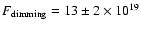 Mx.
Mx.
![\begin{figure}
\par\includegraphics[width=8.5cm,clip]{1079fi8t.ps}\par\vspace*{3mm}
\includegraphics[width=8.5cm,clip]{1079fi8b.ps}
\end{figure}](/articles/aa/full/2005/17/aa1079/Timg40.gif) |
Figure 8:
Top: TRACE 195 Å observation at 00:38 UT on May 11
(reversed color) with two isocontours (grey lines) of the
photospheric field taken with MDI at 00:03 UT (positive:
continuous, negative: dashed). Bottom: the same image with
more isocontours (25, 50, 75, 100, 150, 200,
grey lines) and computed field lines
superimposed (the thin lines have been
computed using
 Mm-1 and the thick
lines using Mm-1 and the thick
lines using
 Mm-1). Notice the global
S shape of the emission, which is a consequence of the
strong non-potentiality of the magnetic field configuration.
Both x and y axes are measured in Mm. Mm-1). Notice the global
S shape of the emission, which is a consequence of the
strong non-potentiality of the magnetic field configuration.
Both x and y axes are measured in Mm. |
| Open with DEXTER |
Coronal observations enable us to identify the few magnetic
flux-tubes which are significantly heated, and therefore are denser
and hotter than the surrounding ones.
But the variable emission along the loops, the multiple loops along the
line-of-sight, and the
limited spatial resolution all contribute to degrade the information.
We can obtain complementary information by computing the coronal
magnetic field. Using MDI magnetograms, we have extrapolated the
observed photospheric line of sight component of the field to the
corona under the linear (or constant  )
force-free field
assumption:
)
force-free field
assumption:
 .
We have
used a fast Fourier transform method as proposed by
Alissandrakis (1981).
.
We have
used a fast Fourier transform method as proposed by
Alissandrakis (1981).
The value of
is chosen so as to best fit
the observed coronal loops at a given time
(Fig. 8). High resolution images are needed to
identify independent loops. They were obtained with TRACE only in a short
time interval before the first X-ray burst.
The value of
is determined through an
iterative process. First, we compute the coronal field assuming a
given value for ,
then we compare the computed field lines to
the observed TRACE coronal loops and, finally, through successive
steps we select the value of
that gives the best global fit
(Green et al. 2002).
As usually found before in other ARs,
is higher in the
core of the region
Mm-1 (thick lines in
Fig. 8) than in the peripheries
Mm-1 (thin lines). We point out that the values of used to model TRACE loops are about ten times higher than any other value we
have used before to model coronal field observations, meaning that the coronal
field is strongly non-potential. The central field lines are S-shaped, while
the surrounding lines are J-shaped. By comparing the magnetic extrapolation
with the observed loops in Fig. 8 we get a better
idea of the highly sheared magnetic configuration.
An important physical quantity to link coronal observations to
interplanetary ones is the magnetic helicity, because it is an
almost conserved quantity.
Once the coronal model is determined, we compute the relative coronal
magnetic helicity,
 ,
following Berger (1985). When
exceeds a certain critical value (
,
following Berger (1985). When
exceeds a certain critical value (
 ), which
depends on the size of the integration box,
may take very
high unphysical values (see Green et al. 2002, mainly their Appendix).
A way to avoid this artificial enhancement of
when
lies close to
,
which is the case for our coronal
model, is to use a linearized version of the expression given by
Berger (1985, see his Eq. (A23)) as discussed in
Green et al. (2002, see their Eq. (11)). We note that there were
typographic errors in the published equation; however,
these typos appeared only in the script
and did not influence the results. The correct expression is:
), which
depends on the size of the integration box,
may take very
high unphysical values (see Green et al. 2002, mainly their Appendix).
A way to avoid this artificial enhancement of
when
lies close to
,
which is the case for our coronal
model, is to use a linearized version of the expression given by
Berger (1985, see his Eq. (A23)) as discussed in
Green et al. (2002, see their Eq. (11)). We note that there were
typographic errors in the published equation; however,
these typos appeared only in the script
and did not influence the results. The correct expression is:
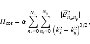 |
(1) |
where the mode
nx=ny=0 (uniform field) has no contribution.
Following this approach, we have obtained the results listed in
Table 1.
When a flux tube is ejected from the solar corona into the
interplanetary medium, it carries part of the magnetic helicity
contained in the coronal field. Therefore, we need to compute the
variation of the coronal magnetic helicity before and after an
eruptive event to compare this coronal global quantity to the
corresponding one in the associated interplanetary event. Unluckily,
TRACE images are only available before the first X-ray burst.
Furthermore, due to the low intensity and spatial resolution of both
SXT and even EIT, it is difficult to distinguish the shape of
individual coronal loops and to use their images to determine the
value of .
Table 1:
Coronal magnetic helicity and its variation. The values
have been computed using MDI magnetograms at the times shown.
This lapse of time includes the three X-ray bursts observed by
SXT (see Sect. 2.3).
The helicity values are in units of 1039 Mx2.
Taking a conservative approach to determine a lower bound for the variation
of the coronal magnetic helicity, we select the closest in time MDI
magnetogram after the third X-ray burst (starting at 8:03 UT) and,
using the previously determined values for ,
we computed
.
The results are shown in the second row of Table 1.
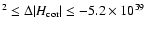
The minimum decrease of
 is in the range of
 Mx
Mx
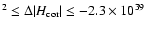 Mx2.
In fact
is expected to decrease after the eruption which implies
a larger decrease of
.
The largest possible variation is obtained if
the magnetic field fully relaxes to a potential configuration after the event.
The latter case
gives:
Mx2.
In fact
is expected to decrease after the eruption which implies
a larger decrease of
.
The largest possible variation is obtained if
the magnetic field fully relaxes to a potential configuration after the event.
The latter case
gives:
 Mx
Mx
 Mx2. The real range for
 should be somewhere in between
the two ranges of values.
should be somewhere in between
the two ranges of values.
We analyze interplanetary data around the expected
time of arrival, 2-5 days later than the coronal event, with
the hope to identify the interplanetary manifestation of
the main sigmoidal eruption observed at 9:00 UT
on 11 May (third X-ray burst). From 10:00 UT on 13 May to
04:00 UT on 16 May, the spacecraft Wind
(located in the vicinity of the Lagrangian point, L1)
observed
low values of the radial velocity ( )
of the solar wind
(300 km s
)
of the solar wind
(300 km s
 km s-1). A very extended
region containing plasma with a high intensity
and disordered magnetic field, and low
proton
km s-1). A very extended
region containing plasma with a high intensity
and disordered magnetic field, and low
proton  (being
the ratio of the plasma to
the magnetic pressure), was also observed by Wind
between 15-17 May, 1998. The signatures just described are
typical of complex interplanetary ejecta. We selected one
minute resolution magnetic data along this period, and found that
the duration of the complex ejecta is around 50 h.
The data
were downloaded from the public site:
http://cdaweb.gsfc.nasa.gov/cdaweb/istp-public/.
(being
the ratio of the plasma to
the magnetic pressure), was also observed by Wind
between 15-17 May, 1998. The signatures just described are
typical of complex interplanetary ejecta. We selected one
minute resolution magnetic data along this period, and found that
the duration of the complex ejecta is around 50 h.
The data
were downloaded from the public site:
http://cdaweb.gsfc.nasa.gov/cdaweb/istp-public/.
Despite the fact that to identify an individual flux rope
within a complex ejecta at 1 AU is highly improbable
(Burlaga et al. 2002), in this particular case we are
able to isolate a small event lasting from 22:00 UT on 15 May to
01:50 UT on 16 May (Fig. 9), around 4 days and
14 h (110 h) after the sigmoidal eruption.
We found this small interplanetary
event by scanning the full temporal evolution
of the ejecta and separating the data in different sections.
Considering an average speed of
 km s-1, we
expect a travel time of
km s-1, we
expect a travel time of
 h from the corona to 1 AU;
then, the small event is a good candidate to be the interplanetary
manifestation of the coronal eruption
since we found a very good agreement with the estimated
delay. The identified interplanetary event shows a large and coherent
rotation of the component
h from the corona to 1 AU;
then, the small event is a good candidate to be the interplanetary
manifestation of the coronal eruption
since we found a very good agreement with the estimated
delay. The identified interplanetary event shows a large and coherent
rotation of the component
 ,
for about 4 h (beginning
and end indicated by dashed vertical lines in the two upper panels of
Fig. 9). This is consistent with the observation of a
cylindrical flux rope as it crosses the Wind spacecraft.
The coherent rotation of the magnetic field vector (Fig. 9,
bottom panel), together with a high magnetic intensity and low proton
temperature, indicate that this small event falls within the definition
of MCs (Burlaga et al. 1981).
This is one of the smallest MCs identified in in situ data
till now. The velocity profile of the cloud (not shown)
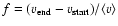
is almost linear with an average velocity (v)
350 km s-1. It is expanding, with an expansion
factor
,
for about 4 h (beginning
and end indicated by dashed vertical lines in the two upper panels of
Fig. 9). This is consistent with the observation of a
cylindrical flux rope as it crosses the Wind spacecraft.
The coherent rotation of the magnetic field vector (Fig. 9,
bottom panel), together with a high magnetic intensity and low proton
temperature, indicate that this small event falls within the definition
of MCs (Burlaga et al. 1981).
This is one of the smallest MCs identified in in situ data
till now. The velocity profile of the cloud (not shown)
is almost linear with an average velocity (v)
350 km s-1. It is expanding, with an expansion
factor
 (
(
 ).
).
![\begin{figure}
\par\includegraphics[width=8.8cm,clip]{1079fi9t.ps}\par\vspace*{3mm}
\includegraphics[width=8.8cm,clip]{1079fi9b.ps}
\end{figure}](/articles/aa/full/2005/17/aa1079/Timg60.gif) |
Figure 9:
Interplanetary magnetic field data obtained
by the Wind spacecraft. The two upper panels show
the complex ejecta (with the small MC located in between
the dashed lines), and the three lower panels are a
zoom on the small MC. We plot the magnetic
field intensity (|B|) and its components
in Geocentric Solar Ecliptic (GSE) coordinates as
a function of time. |
| Open with DEXTER |
When modeling an MC, we need to define a system of coordinates fixed to
the cloud. Assuming that the MC has a cylindrical helical magnetic structure, the
natural coordinates to describe its magnetic field are the polar ones
(r,  ,
z), such that
,
z), such that
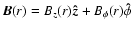 .
We can define a cartesian system of coordinates fixed to the cloud, such
that
.
We can define a cartesian system of coordinates fixed to the cloud, such
that
 is parallel to the axis of the cloud and
Bz is positive at this axis.
is parallel to the axis of the cloud and
Bz is positive at this axis.
 is the unit vector defined by the projection of the spacecraft trajectory
orthogonal to
,
and
is the unit vector defined by the projection of the spacecraft trajectory
orthogonal to
,
and
 is such that the system is right-handed.
When the spacecraft's path intersects the axis of the ideal cloud defined
above, the magnetic field data obtained by the spacecraft will show:
 ,
a large and coherent variation of
,
a large and coherent variation of
 from positive to negative (or from negative to positive, depending on the
sign of the magnetic helicity), and an intermediate and coherent variation
of
from positive to negative (or from negative to positive, depending on the
sign of the magnetic helicity), and an intermediate and coherent variation
of
 ,
from low values at one cloud edge, taking the
largest value at its axis and returning to low values at the other edge
(Bothmer & Schwenn 1998).
,
from low values at one cloud edge, taking the
largest value at its axis and returning to low values at the other edge
(Bothmer & Schwenn 1998).
We determine the orientation of the observed magnetic cloud using a minimum
variance (MV) analysis of the magnetic observations (Sonnerup & Cahill 1967).
This method finds the direction (
 )
in which the mean
quadratic deviation of the field,
)
in which the mean
quadratic deviation of the field,
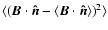 ,
is minimum (maximum). It is
possible to show that this is equivalent to finding the eigen-vector
corresponding to the smallest (highest) eigenvalue of the covariance matrix
,
is minimum (maximum). It is
possible to show that this is equivalent to finding the eigen-vector
corresponding to the smallest (highest) eigenvalue of the covariance matrix
 .
As we mentioned above, when the minimum
distance from the spacecraft to the axis of the flux tube is close to zero,
the largest (resp. smallest) change of
.
As we mentioned above, when the minimum
distance from the spacecraft to the axis of the flux tube is close to zero,
the largest (resp. smallest) change of  comes from the
component of the field associated with By (resp. Bx).
Thus, this MV method determines the direction of the maximum
(
), intermediate
(
), and minimum
(
)
variance of the field. A more complete
discussion of the MV method applied to interplanetary flux tubes can be
found in the appendix of Bothmer & Schwenn (1998).
comes from the
component of the field associated with By (resp. Bx).
Thus, this MV method determines the direction of the maximum
(
), intermediate
(
), and minimum
(
)
variance of the field. A more complete
discussion of the MV method applied to interplanetary flux tubes can be
found in the appendix of Bothmer & Schwenn (1998).
In our event, we find a well-defined direction for the axis of the MC
(corresponding to the intermediate eigen-vector) since we get an
intermediate to minimum eigenvalues ratio of 6. We define the MC axis
orientation as follows: the angle  between the ecliptic plane and
the MC axis, and the angle
between the ecliptic plane and
the MC axis, and the angle  between
 and
the projection of the MC axis on the ecliptic plane (measured positive when
counterclockwise). We find that
and
the projection of the MC axis on the ecliptic plane (measured positive when
counterclockwise). We find that
 and
and
 ,
so the projection of the axis of the cloud on the ecliptic
plane lies almost along
;
in particular, with the
magnetic field pointing towards
,
so the projection of the axis of the cloud on the ecliptic
plane lies almost along
;
in particular, with the
magnetic field pointing towards
 .
.
In this approach, the spacecraft impact parameter (the
minimum distance from the spacecraft trajectory to the axis of the cloud),
p, is not
determined and we set it equal to zero, noting that the large angle rotation
of the field (147 ,
see left upper panel of
Fig. 10) indicates that the ratio between the impact
parameter and the radius of the cloud (p/R) should be small. This field
rotation also implies that the sign of the helicity is negative. Next, from
the measured velocity, the spacecraft trajectory through the cloud
and the time along which
Wind observed the cloud, we estimate a radius
,
see left upper panel of
Fig. 10) indicates that the ratio between the impact
parameter and the radius of the cloud (p/R) should be small. This field
rotation also implies that the sign of the helicity is negative. Next, from
the measured velocity, the spacecraft trajectory through the cloud
and the time along which
Wind observed the cloud, we estimate a radius
 AU, which implies a very small MC.
![\begin{figure}
\par\includegraphics[width=8.8cm,clip=]{1079f10t.ps}\par\vspace*{3mm}
\includegraphics[width=8.8cm,clip=]{1079f10b.ps}
\par\end{figure}](/articles/aa/full/2005/17/aa1079/Timg79.gif) |
Figure 10:
Magnetic field components in local MC coordinates.
The two upper panels show the hodograms for the MC.
The central and lower panels show the evolution of the
magnetic field components (with the orientation of the cloud
given by the minimum variance method, see
Sect. 4.2).
The observed magnetic data are drawn with thick
lines, and the best solutions fitted using Lundquist's model
are shown with thin lines. |
| Open with DEXTER |
In situ measurements of interplanetary magnetic flux tubes at 1
AU are consistent with several axially symmetric magnetic field
models. The most frequently used is the linear force-free model
of Lundquist (1950),
,
with
constant
(e.g., Burlaga et al. 1981; Burlaga 1988; Lepping et al. 1990). For
helical-cylindrical configurations
of the field, the amount by which a given field line is twisted per
unit length, i.e., the twist
 ,
depends only on r. In particular for the Lundquist's model, the
twist when
,
depends only on r. In particular for the Lundquist's model, the
twist when  0 is
0 is
 .
A cylindrical non-linear force-free field with a uniform twist,
i.e.
.
A cylindrical non-linear force-free field with a uniform twist,
i.e.
 (Gold & Hoyle 1960), is also
used to model interplanetary flux tubes
(e.g., Farrugia et al. 1999).
The cylindrical non force-free model proposed by
Hidalgo et al. (2002,2000) assumes a constant current density
such that
(Gold & Hoyle 1960), is also
used to model interplanetary flux tubes
(e.g., Farrugia et al. 1999).
The cylindrical non force-free model proposed by
Hidalgo et al. (2002,2000) assumes a constant current density
such that
 ,
where
,
where  and jz are constants.
The magnetic field of these three different cylindrical flux tube
configurations can be obtained as a function of r (the radius),
B0 (the field at the flux tube axis), and  (the twist at the flux
tube axis), for detailed expressions see Dasso et al. (2003b).
(the twist at the flux
tube axis), for detailed expressions see Dasso et al. (2003b).
We use the orientation found from the MV method to model the observed
field, according to the three models described above, and we obtain the two
physical parameters (
 )
that best fit the observations following
the method discussed in Dasso et al. (2003a,b). The two lower
panels in Fig. 10 correspond to
and
for the small MC. The observed data are shown with thick
lines and the curves obtained using the parameters fitted to the Lundquist's
model are shown with thin lines. The other two models (Gold-Hoyle &
Hidalgo et al.) give similar curves.
)
that best fit the observations following
the method discussed in Dasso et al. (2003a,b). The two lower
panels in Fig. 10 correspond to
and
for the small MC. The observed data are shown with thick
lines and the curves obtained using the parameters fitted to the Lundquist's
model are shown with thin lines. The other two models (Gold-Hoyle &
Hidalgo et al.) give similar curves.
Table 2 shows the fitted values for
and B0
for the three models. The value of B0 is very similar in the three
models (14-16 nT). The twist of the field lines at the center
of the tube is lower for Hidalgo's et al. model and larger (70% with respect to its lowest value) for Gold-Hoyle's model.
Magnetic flux and magnetic helicity (
 )
are
two important global physical quantities that characterize the magnetic field
configuration in interplanetary clouds. They are also useful to link
interplanetary events to their coronal
source region.
)
are
two important global physical quantities that characterize the magnetic field
configuration in interplanetary clouds. They are also useful to link
interplanetary events to their coronal
source region.
Using the three models described in the previous section, we can find
analytical expressions for the flux (Fz) of Bz
(i.e., along the flux tube) and also for the flux
(
 )
of
)
of  per unit length along the MC.
The value of Fz can be computed directly from the distribution of
Bz for every model. Concerning
per unit length along the MC.
The value of Fz can be computed directly from the distribution of
Bz for every model. Concerning
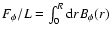
 ,
for the Lundquist's model, we
have:
,
for the Lundquist's model, we
have:
![$F_{\phi}^L/L = B_0 [1-J_0(\alpha R)]/\alpha$](/articles/aa/full/2005/17/aa1079/img89.gif) ,
where J0
is the Bessel function of the first kind and zero order. For the Gold-Hoyle
model, we
find:
,
where J0
is the Bessel function of the first kind and zero order. For the Gold-Hoyle
model, we
find:
 .
While,
for the Hidalgo's et al. model, we have:
.
While,
for the Hidalgo's et al. model, we have:
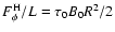 .
.
Table 2:
Geometrical (obtained from the minimum variance method)
and physical parameters (fitted with a least-square method)
for the small MC. L, G, and H refer to Lundquist, Gold
and Hoyle, and Hidalgo et al. model, respectively.
The geometrical parameters are:
the angle
between the axis of the tube and the ecliptic
plane, the angle
between the projection of the axis on the
ecliptic plane and the abscissa of GSE (anti-clockwise as seen from
the positive
 axis), and the flux tube radius (R).
The two physical parameters are:
the twist per unit length ()
and
the intensity of the field (B0), both at the flux tube centre.
In the last three columns,
we give the computed magnetic flux in the Bz component
(Fz), in the
component per unit length
(
)
and the magnetic helicity per unit length
(
axis), and the flux tube radius (R).
The two physical parameters are:
the twist per unit length ()
and
the intensity of the field (B0), both at the flux tube centre.
In the last three columns,
we give the computed magnetic flux in the Bz component
(Fz), in the
component per unit length
(
)
and the magnetic helicity per unit length
(
 ).
).
In a cylindrical magnetic field configuration, a simple
expression for the relative helicity content per unit length in the cloud is
given by:
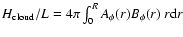 ,
where
,
where  is the component
 of the potential
vector.
Thus, for the Lundquist's model, the helicity writes:
of the potential
vector.
Thus, for the Lundquist's model, the helicity writes:
 ,
where J1 is the Bessel function of the first kind and
first order. The variables
,
where J1 is the Bessel function of the first kind and
first order. The variables
 and
and
 are
dimensionless quantities. For the Gold-Hoyle model, the helicity is
given by:
are
dimensionless quantities. For the Gold-Hoyle model, the helicity is
given by:
![$H_{\rm cloud}^{\rm G}/L
= ( 8\pi [\ln(1+ U^2/4)]^2 U^{-4} )
B_0^2 R^4 \tau_0$](/articles/aa/full/2005/17/aa1079/img98.gif) .
Finally, for the Hidalgo's et al. model we have:
.
Finally, for the Hidalgo's et al. model we have:
 .
.
The magnetic flux of Bz has a narrow range of values in the
force-free cases (seventh column in Table 2),
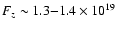 Mx, but it changes by - 30% for
Hidalgo's et al. model. Fz for this small MC is about one hundredth of
the average value for large MCs (
Mx, but it changes by - 30% for
Hidalgo's et al. model. Fz for this small MC is about one hundredth of
the average value for large MCs (
 Mx). The same
behaviour is found for the magnetic flux of
per unit length
for the two force-free models,
Mx). The same
behaviour is found for the magnetic flux of
per unit length
for the two force-free models,
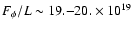 Mx/AU; while it changes only
by 15% for Hidalgo's et al. model.
Mx/AU; while it changes only
by 15% for Hidalgo's et al. model.
The magnetic field of the flux tube is left-handed so
is
negative, and it is in the range
 Mx2/AU for the three models (last column in
Table 2). Note that the two force-free models give practically
the same magnetic helicity, while the non-force free model gives a lower
value for
Mx2/AU for the three models (last column in
Table 2). Note that the two force-free models give practically
the same magnetic helicity, while the non-force free model gives a lower
value for
 by 7%. The magnetic helicity per
unit length for this event is smaller than for typical MCs by three orders of
magnitude, being the mean value of the helicity in clouds
by 7%. The magnetic helicity per
unit length for this event is smaller than for typical MCs by three orders of
magnitude, being the mean value of the helicity in clouds
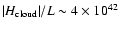 Mx2/AU (van-Driel Gesztelyi et al. 2003).
In Sect. 3 we have shown that the small AR at disc
centre on 11 May 1998 produced three main X-ray bursts. The third one was
the most significant in X-ray total flux, in EUV evolution and also in
evidences for eruption. This coronal eruption and the interplanetary MC,
described in Sect. 4, have properties that indicate
their probable association:
- -
- Location: eruption very close to the disc centre; as ejections travel
dominantly in the radial direction it implies that the event could
be observed by Wind.
- -
- Timing: four and half days travel time what is expected for a slow CME
travelling at about the speed of the slow solar wind
(e.g., Vrsnak & Gopalswamy 2002) as measured in situ by Wind.
- -
- The orientation of the MC axis is approximately the same as the
direction of the elongated coronal sigmoid. Furthermore, the
signs of the axial magnetic field in the MC and of the AR polarities
are the same.
- -
- The sign of the magnetic helicities of the MC and the small AR are in
agreement.
Any of the above correspondences between the physical characteristics
on the Sun and in the interplanetary medium could happen by chance.
However, the probability that all
these characteristics coincide simultaneously just by chance is
small. We conclude that the observed small MC is most
probably the consequence of the observed coronal eruption.
This is summarized in Fig. 11.
Furthermore, from the interplanetary magnetic field (Fig. 9),
the orientation of the MC
and the geometry
of the coronal magnetic field (Fig. 8), we can
deduce that the Wind spacecraft crossed the positive (western) leg of the
flux rope. This is coherent with the position of the small active region
at the time of the eruption (2 degrees of longitude East on the Sun) if the
ejection occurred mostly in the radial direction.
Several ARs were present on the Sun at the time of our X-ray bursts
and a number of flares in the high-B to low-C GOES range occurred from May 11
to May 12 (see http://www.sec.noaa.gov/weekly/pdf1998/prf1185.pdf). The
third X-ray burst discussed here could be identified as the B6.9 GOES event
reported by
NOAA that was not associated to any of the numbered ARs on the disc
and reached maximum at 09:03 UT.
Within the next 34 h there were 7 more flare events, 5 of them slightly more
intense, while the other two of similar magnitude as the third X-ray burst.
Of these events,
the B8.4 flare starting on 11 May at 12:54 UT and the C1.2 flare starting on
12 May at 05:07 UT can be regarded as long-duration events, which are usually
thought to be eruptive (see some examples in van Driel-Gesztelyi et al. 2000).
However, these two events (as most of the events during 11 and 12 May)
occurred in AR 8218, which was located at S20E15 on 11 May at
08:00 UT (see Fig. 1). The loops in AR 8218, as those in another
decaying not numbered AR located at S25W20,
had a global forward
S-shape which is considered as an indication of positive
twist (see Pevtsov & Balasubramaniam 2003, and references therein). Since the SXT image in
Fig. 1 has been enhanced in order to better show the
small bright point, saturating brighter loops, we refer the reader to
http://surfwww.mssl.ucl.ac.uk/surf/sxt/images/sxt_980511.120226.gif
for a better view of the loops in AR 8218. This positive twist in southern
hemisphere ARs is what is expected according to the hemispheric chirality
rules (Pevtsov & Balasubramaniam 2003). Therefore, none of the events occurring in AR 8218
could have given origin to the small MC observed by Wind, which had a negative
magnetic helicity.
Concerning the orientation of the elongated coronal sigmoid, if the
flux tube goes through a kink instability during the eruption
(as suggested by some numerical simulations, see e.g. Török & Kliem 2004; Fan & Gibson 2003)
part of the negative twist would be traded for a negative writhe; this will
turn the flux tube axis clockwise.
However, we have no evidence that the
ejected flux tube was kinked and, furthermore, numerical
simulations do not follow the evolution in the interplanetary space.
Moreover, we concluded that the spacecraft crossed the western leg
of the flux rope (i.e., the calculated MC orientation corresponds to
the orientation of that portion of the flux tube);
so, the orientation of the leading part of the flux rope is not known.
![\begin{figure}
\par\includegraphics[width=8.8cm,clip]{1079f11.eps}
\end{figure}](/articles/aa/full/2005/17/aa1079/Timg106.gif) |
Figure 11:
Schematic global view of the magnetic cloud and its
source region (notice that in this figure the solar North is to
the left). The MC leading part is represented by continuous lines,
while dashed lines are used closer to the Sun since, considering the
photospheric magnetic observations, the MC should be
detached from its solar source by the time it was observed by the
Wind spacecraft. |
| Open with DEXTER |
Next, we attempt to quantify this link with the measured magnetic fluxes
and helicities. For the comparison of the coronal and interplanetary
magnetic helicities, the main unknown is the distribution of the twist
along the interplanetary
flux rope. Even supposing a uniform distribution, the MC length is unknown.
In large-scale
MCs, there is frequently evidence of their magnetic connection to the Sun
when they are observed at 1 AU (e.g. presence of bi-streaming electrons).
This leads to an MC length slightly larger than 2 AU. However, for the studied
MC, we know that the photospheric magnetic bipole disappeared about one day
after the eruption (Fig. 2), so the erupting flux rope
was well detached from its original solar source when it was observed
in situ 4.5 days after the coronal eruption. A simple
proportionality gives a length of 0.5 AU. However, after reconnection
with large-scale field lines, the magnetic twist contained in the ejected
flux tube propagates along the new connections as a torsional Alfvén wave.
Taking a typical Alfvén velocity of 100 km s-1, the twist can
propagate on both sides of the flux tube over a length of 0.2 AU in
3.5 days. We conclude that the probable length of the observed MC is
between 0.5 and 1 AU.
![\begin{figure}
\par\includegraphics[width=7cm,clip=]{1079f12t.eps}\par\vspace*{3mm}
\includegraphics[width=7cm,clip=]{1079f12b.eps}
\end{figure}](/articles/aa/full/2005/17/aa1079/Timg107.gif) |
Figure 12:
A sketch showing the way a magnetic flux tube
can be formed by magnetic reconnection in an expanding sheared arcade
(Démoulin et al. 1996). The upper and lower figures
show two field lines belonging to the expanding
arcade ( top), and a small arcade and flux tube ( bottom), before
and after reconnection respectively. PIL indicates the photospheric
inversion line. Further reconnection between the
flux tube and the large scale
arcade will increase the number of turns in the flux
tube.
Coronal dimmings are expected to form in all the expanding
arcade. However, only a
fraction of the photospheric flux of the dimmings contributes to
the longitudinal flux of the twisted flux tube; the remaining part is
transferred (through reconnection) to the magnetic flux in the azimuthal
component. |
| Open with DEXTER |
We found that the flux in the dimmings is
Mx. To which of the two flux values
computed for the MC should this value be compared will depend on the way the
ejection occurs. If the MC would result from a simple expansion of coronal
loops, then
 would correspond to the flux of the axial field component of
the MC (Bz). However, we have found that Fz is
only one tenth of
.
If the ejection is the result of the
expulsion of a twisted flux tube formed during the eruption by successive
reconnections in a sheared magnetic arcade (as suggested by Démoulin et al. 1996; Titov & Démoulin 1999, see a
sketch in Fig. 12), which we consider
as the plausible scenario in our case (see the discussion in
Sect. 2.5); then,
should be closer to the value of the flux in the azimuthal
component of the cloud (). The value of
is in the range 19 to
would correspond to the flux of the axial field component of
the MC (Bz). However, we have found that Fz is
only one tenth of
.
If the ejection is the result of the
expulsion of a twisted flux tube formed during the eruption by successive
reconnections in a sheared magnetic arcade (as suggested by Démoulin et al. 1996; Titov & Démoulin 1999, see a
sketch in Fig. 12), which we consider
as the plausible scenario in our case (see the discussion in
Sect. 2.5); then,
should be closer to the value of the flux in the azimuthal
component of the cloud (). The value of
is in the range 19 to
 Mx AU-1. Considering a length
between 0.5
and 1 AU for the cloud, we find:
Mx AU-1. Considering a length
between 0.5
and 1 AU for the cloud, we find:
 Mx
Mx
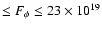 Mx, so
  is in
good agreement with
.
is in
good agreement with
.
The estimated cloud helicity is
 to
to
 Mx2, so in the range of 0.5-1.3 the
variation of helicity found at the coronal level (
in
Table 1). These values are also in good agreement.
Mx2, so in the range of 0.5-1.3 the
variation of helicity found at the coronal level (
in
Table 1). These values are also in good agreement.
From the common properties between the magnetic configuration in the corona
and the interplanetary space (listed in the first paragraph of this section),
but also evidenced by the same order of
magnetic fluxes and helicities, we
conclude that
the observed coronal eruption (third X-ray burst in
Fig. 2) was indeed observed in the interplanetary space
as a small MC. Such link could be found for such a tiny event mostly because
the small AR was well isolated at disc centre, but also because a large
variety of complementary solar observations, with a good time coverage, were
available.
![\begin{figure}
\par\includegraphics[width=8.5cm,clip]{1079f13.ps}
\end{figure}](/articles/aa/full/2005/17/aa1079/Timg115.gif) |
Figure 13:
Comparison to the event studied by
Manoharan et al. (1996). The left (resp. right) column
correspond to X-ray images at the beginning (resp. after)
the eruption. The top row shows the studied X-ray bright point,
as observed in SXT full disc images (the field of view is about
 arcsec).
The middle and bottom rows are the SXT partial frame images
of the event studied by Manoharan et al. (the field of view is about arcsec).
The middle and bottom rows are the SXT partial frame images
of the event studied by Manoharan et al. (the field of view is about
 arcsec). The original images
are shown in the bottom row, while their spatial resolution has been
degraded (rebinned) by a factor 8 in
the middle row (to account both for the difference in the observed
resolution, a factor 2, and spatial extension of the ARs, about
a factor 4). arcsec). The original images
are shown in the bottom row, while their spatial resolution has been
degraded (rebinned) by a factor 8 in
the middle row (to account both for the difference in the observed
resolution, a factor 2, and spatial extension of the ARs, about
a factor 4). |
| Open with DEXTER |
The studied small AR, observed from 10 to 12 May 1998 by SOHO, TRACE
and Yohkoh, was especially interesting for the following reasons. First,
its full evolution, from birth to full disappearance, could be observed close
to the disc centre. Second, it contrasts with previous studies by its
lifetime and the amount of its magnetic flux since both are a factor one hundred
lower than in earlier full-evolution studies of ARs (Démoulin et al. 2002; Green et al. 2002).
Third, it is a simple and isolated magnetic bipole, well separated from
other ARs (by at least half solar radius) but it was still eruptive. Finally,
an associated magnetic cloud (MC) could be identified in the interplanetary
medium; this MC is also a factor
one hundred smaller (in magnetic flux) than most MCs analyzed so far.
The history of this small AR can be briefly summarized as follows.
The evolution of the photospheric magnetic field is consistent with
the emergence of a strongly twisted  loop. The coronal EUV and X-ray
emissions
show elongated S-shaped structures situated along
the magnetic inversion line
of the photospheric bipole; this characterizes a
strongly non-potential
coronal magnetic field. Three major X-ray bursts occurred during the AR's
lifetime. All of them
are associated with a shortening of the coronal loops, which
characterizes a relaxation to a lower magnetic energy state. Two of these
bursts are associated with observed dimmings in EUV. Only the third burst
is associated with the formation of a cusp in the EUV emission.
This third burst also shows the most important change of shape in the EUV
and the most extended dimmings (with two extended lobes); therefore,
we conclude that
this event was the largest eruption of this small AR.
loop. The coronal EUV and X-ray
emissions
show elongated S-shaped structures situated along
the magnetic inversion line
of the photospheric bipole; this characterizes a
strongly non-potential
coronal magnetic field. Three major X-ray bursts occurred during the AR's
lifetime. All of them
are associated with a shortening of the coronal loops, which
characterizes a relaxation to a lower magnetic energy state. Two of these
bursts are associated with observed dimmings in EUV. Only the third burst
is associated with the formation of a cusp in the EUV emission.
This third burst also shows the most important change of shape in the EUV
and the most extended dimmings (with two extended lobes); therefore,
we conclude that
this event was the largest eruption of this small AR.
The above summary indicates that the third event has all the observational
signatures of classical eruptive events. We compare its X-ray evolution
to a
large-scale case (extending to one solar radius) analyzed by
Manoharan et al. (1996). In both cases the magnetic bipole was mostly East-West
with an inversion line slightly inclined in the North-South direction, and
both cases
have negative magnetic helicity (inverse-S shaped coronal
emission). The high-resolution observations (SXT partial frame) of the
25 October 1994 event let us
identify two sets of bright loops: long, sigmoidal ones
and short, sheared ones (Fig. 13, bottom left). Mainly the
short ones, analogous to classical flare loops, remain later on in the event
(Fig. 13, bottom right). The sigmoidal loops progressively
decrease in brightness as they expand (implying a decrease of plasma
density and, then, of emission). There has most probably been
an ejection towards the
interplanetary space, but the associated CME could not be identified because
observations were not available. These high-resolution observations
let us characterize
the reconnection process among the sheared loops of the
bipole: as the ejection took place, the reconnection enlarged
(or at least
formed) a twisted flux tube; the new reconnected loops can be identified as the
sigmoidal and short loops (see e.g. Démoulin et al. 1996). The presence
of two sets of loops is much less obvious if we simply degrade the original
images to meet the observing conditions of the much smaller 11 May 1998 event
(Fig. 13, middle row). Here, we mainly observe the transition
from an
elongated X-ray emission (with a brighter core) to a compact emission. This
is the main characteristic of the 11 May event (Fig. 13, top
row). We conclude that we have basically the same phenomenon, but
rescaled. The main difference between the two top rows of
Figure 13, the contrast of the sigmoidal loops, is likely to be
a direct effect of the scaling: in the 11 May case there is much less
energy release involved; so, cooler but also much less dense coronal
loops were formed, both effects contributing to a lower emission in the
SXT detection range.
In the interplanetary medium, we plausibly find the associated ejecta
because it shares the characteristics expected for an eruption from the small
AR (Sect. 5). This small MC is also a small-scale
version of previously observed
classical MCs (even if it is embedded in a much larger event). This broadens
our view of solar eruptions: they could also be of small scale. Indeed,
taking into account the frequency of small scale bipoles on the Sun, we
expect that such small ejected flux tubes would be relatively frequent in the
interplanetary space (while present studies are biased by focusing
on large-scale events, which are easier
to identify). The relative global importance of these
small-scale events in terms of magnetic flux, energy and helicity, remains
to be investigated.
Such small events present a challenge for CME models,
which have been developed for large scale magnetic configurations.
However, since the event is very small and not fully covered
by high spatial and temporal
resolution data, a confrontation with any current CME
model is difficult and, then, non-conclusive. Such confrontation would
need a 3D MHD simulation of the event.
Still, the analyzed event brings two constraints.
First, the observations show that the
magnetic stress is brought with the magnetic field by emergence and
not by shearing motions due to differential rotation, which inputs a
negligible amount
of helicity on a time scale of one day. This confirms previous results
obtained on classical ARs (Chae et al. 2001; Nindos & Zhang 2002; Démoulin et al. 2002; Green et al. 2002).
Second, the comparison of the magnetic fluxes indicates that an important
fraction of the ejected flux rope is formed by reconnection
of sheared arcade-like
field lines.
Finally, to understand better this kind of small events, we certainly need
coronal observations with both a better sensitivity (dynamic range)
and spatial resolution. The next missions, Solar B and Solar Orbiter,
are well suited to continue this research. Moreover, observing the
associated CME is still a challenge. The configuration of the two
spacecrafts of STEREO would allow us to observe such event also from a
lateral point of view, from which it is easier to detect the scattered
light of such a small halo CME.
Acknowledgements
The authors thank the referee, B. Kliem, for very constructive comments
on the paper. The authors thank the SOHO/MDI and EIT consortia
for their data, the Mullard Space Science Laboratory (MSSL) Solar UK
Research Facility (SURF) for YOHKOH/SXT, and the NASA's Space Physics
Data Facility (SPDF) for the interplanetary observations. The Nobeyama
Radioheliograph is operated by Nobeyama Radio Observatory/NAOJ.
SOHO is a joint project by ESA and NASA.
S.P. acknowledges a joint travel grant from CIMO (Finland) and EGIDE
(France).
P.D. and C.H.M. acknowledge financial support from ECOS (France) and
SECyT (Argentina) through their cooperative science program (A01U04).
C.H.M. and L.v.D.G. thank TET (Hungary)
and SECyT for financial support through their cooperation program
(AR03/02 and HU/A01/UIII/01).
P.D. and L.v.D.G. acknowledge travel support from the Royal Society
Joint project (MSSL/UCL-Observatoire de Paris-Meudon).
C.H.M. is grateful for an MSSL/UCL visitor's grant.
S.D. thanks the Observatoire de Paris, Meudon, for support during his
visit.
L.v.D.G. was supported by the Hungarian Government grant OTKA
T-038013. C.H.M. and S.D. thank the Argentinean
grants: UBACyT X329, PIP 2693 and PIP 2388 (CONICET),
and PICT 12187 and PICT 14163 (ANPCyT).
-
Alissandrakis, C. E. 1981, A&A, 100, 197 [NASA ADS] (In the text)
- Antiochos,
S. K., Devore, C. R., & Klimchuk, J. A. 1999,
ApJ, 510, 485 [NASA ADS] [CrossRef] (In the text)
- Berger, M. A.
1985, ApJS, 59, 433 [NASA ADS] [CrossRef] (In the text)
- Berger, T. E.,
& Lites, B. W. 2003, Sol. Phys., 213, 213 [NASA ADS] [CrossRef] (In the text)
- Bothmer, V.,
& Schwenn, R. 1994, Space Sci. Rev., 70, 215 [NASA ADS] [CrossRef]
- Bothmer, V.,
& Schwenn, R. 1998, Ann. Geophys., 16, 1 [NASA ADS] (In the text)
- Burlaga, L.,
Sittler, E., Mariani, F., & Schwenn, R. 1981, J. Geophys. Res.,
86, 6673 [NASA ADS] (In the text)
- Burlaga,
L. F. 1988, J. Geophys. Res., 93, 7217 [NASA ADS]
- Burlaga,
L. F., Plunkett, S. P., & St. Cyr, O. C.
2002, J. Geophys. Res. (Space Physics), 107, 1266 [NASA ADS] (In the text)
- Canfield,
R. C., Hudson, H. S., & McKenzie, D. E. 1999,
Geophys. Res. Lett., 26, 627 [NASA ADS] [CrossRef]
- Chae, J., Wang, H.,
Qiu, J., et al. 2001, ApJ, 560, 476 [NASA ADS] [CrossRef]
-
Démoulin, P., Priest, E. R., & Lonie, D. P.
1996, J. Geophys. Res., 101, 7631 [NASA ADS] [CrossRef] (In the text)
-
Démoulin, P., Mandrini, C. H., van Driel-Gesztelyi, L.,
et al. 2002, A&A, 382, 650 [EDP Sciences] [NASA ADS] [CrossRef]
- Dasso, S.,
Mandrini, C. H., & Démoulin, P. 2003a, in Solar Wind
Ten, AIP Conf. Proc., 546, 786
- Dasso, S.,
Mandrini, C. H., Démoulin, P., & Farrugia, C. J.
2003b, J. Geophys. Res. (Space Physics), 108, 1362 [NASA ADS] (In the text)
-
Delaboudiniere, J.-P., Artzner, G. E., Brunaud, J.,
et al. 1995, Sol. Phys., 162, 291 [NASA ADS] [CrossRef] (In the text)
- Dobrzycka, D.,
Raymond, J. C., Biesecker, D. A., Li, J., &
Ciaravella, A. 2003, ApJ, 588, 586 [NASA ADS] [CrossRef]
- Fan, Y., & Gibson,
S. E. 2003, ApJ, 589, L105 [NASA ADS] [CrossRef] (In the text)
- Farrugia,
C. J., Janoo, L. A., Torbert, R. B., et al.
1999, in Solar Wind Nine, AIP Conf. Proc., 471, 745
(In the text)
- Fisher, G. H.,
Longcope, D. W., Metcalf, T. R., & Pevtsov,
A. A. 1998, ApJ, 508, 885 [NASA ADS] [CrossRef] (In the text)
- Gibson, S. E.,
& Low, B. C. 1998, ApJ, 493, 460 [NASA ADS] [CrossRef] (In the text)
- Gibson, S. E.,
& Low, B. C. 2000, J. Geophys. Res., 105,
18187 [NASA ADS] [CrossRef] (In the text)
- Gibson, S. E.,
Fan, Y., Mandrini, C. H., Fisher, G., & Démoulin, P.
2004, ApJ, 617, 600 [NASA ADS] [CrossRef] (In the text)
- Gilbert,
H. R., Serex, E. C., Holzer, T. E., MacQueen,
R. M., & McIntosh, P. S. 2001, ApJ, 550, 1093 [NASA ADS] [CrossRef]
- Glover, A., Ranns,
N. D. R., Harra, L. K., & Culhane, J. L.
2000, Geophys. Res. Lett., 27, 2161 [NASA ADS] [CrossRef]
- Gold, T., &
Hoyle, F. 1960, MNRAS, 120, 89 [NASA ADS] (In the text)
- Golub, L. 1980, Royal
Society of London Philosophical Transactions Series A, 297,
595 [NASA ADS]
- Green, L. M.,
López Fuentes, M. C., Mandrini, C. H., et al.
2002, Sol. Phys., 208, 43 [NASA ADS] [CrossRef] (In the text)
- Handy, B. N.,
Acton, L. W., Kankelborg, C. C., et al. 1999,
Sol. Phys., 187, 229 [NASA ADS] [CrossRef] (In the text)
- Harrison,
R. A., Bryans, P., & Bingham, R. 2001, A&A, 379,
324 [EDP Sciences] [NASA ADS] [CrossRef]
- Harvey, K. L.
1993, Ph.D. Thesis
- Harvey, K. L.
1997, in Magnetic Reconnection in the Solar Atmosphere, ASP Conf.
Ser., 111, 9
(In the text)
- Hidalgo,
M. A., Cid, C., Medina, J., & Viñas, A. F. 2000,
Sol. Phys., 194, 165 [NASA ADS] [CrossRef]
- Hidalgo,
M. A., Cid, C., Medina, J., Viñas, A. F., &
Sequeiros, J. 2002, J. Geophys. Res., 107
- Howard,
R. A., Sheeley, N. R., Michels, D. J., & Koomen,
M. J. 1985, J. Geophys. Res., 90, 8173 [NASA ADS]
- Kliem, B., Titov,
V. S., & Török, T. 2004, A&A, 413, L23 [EDP Sciences] [NASA ADS] [CrossRef] (In the text)
- López Fuentes,
M. C., Démoulin, P., Mandrini, C. H., &
van Driel-Gesztelyi, L. 2000, ApJ, 544, 540 [NASA ADS] [CrossRef] (In the text)
- López Fuentes,
M. C., Démoulin, P., Mandrini, C. H., Pevtsov,
A. A., & van Driel-Gesztelyi, L. 2003, A&A, 397,
305 [EDP Sciences] [NASA ADS] [CrossRef] (In the text)
- Lepping,
R. P., Burlaga, L. F., & Jones, J. A. 1990, J.
Geophys. Res., 95, 11957 [NASA ADS]
- Lin, J., & Forbes,
T. G. 2000, J. Geophys. Res., 105, 2375 [NASA ADS] [CrossRef] (In the text)
- Lundquist, S.
1950, Ark. Fys., 2, 361 [MathSciNet] (In the text)
- Manoharan,
P. K., van Driel-Gesztelyi, L., Pick, M., & Démoulin,
P. 1996, ApJ, 468, L73 [NASA ADS] [CrossRef] (In the text)
- Marubashi, K.
1997, in Coronal Mass Ejections, Geophysical Monograph, 99,
147
- Mikic, Z., &
Linker, J. A. 1994, ApJ, 430, 898 [NASA ADS] [CrossRef] (In the text)
- Munro, R. H.,
& Sime, D. G. 1985, Sol. Phys., 97, 191 [NASA ADS] [CrossRef]
- Nindos, A., &
Zhang, H. 2002, ApJ, 573, L133 [NASA ADS] [CrossRef]
- Nishio, M.,
Nakajima, H., Enome, S., et al. 1994, in Proc. Kofu Symp.,
19
(In the text)
- Pevtsov,
A. A., & Balasubramaniam, K. S. 2003, Adv. Space
Res., 32, 1867 [NASA ADS] [CrossRef] (In the text)
- Pevtsov,
A. A., Canfield, R. C., & Zirin, H. 1996, ApJ, 473,
533 [NASA ADS] [CrossRef] (In the text)
- Pevtsov,
A. A., Fisher, G. H., Acton, L. W., et al.
2003, ApJ, 598, 1387 [NASA ADS] [CrossRef] (In the text)
-
Pohjolainen, S. 2000, A&A, 361, 349 [NASA ADS] (In the text)
- Rust, D. M. 1994,
Geophys. Res. Lett., 21, 241 [NASA ADS] [CrossRef]
- Rust, D. M., &
Kumar, A. 1996, ApJ, 464, L199 [NASA ADS] [CrossRef] (In the text)
- Scherrer,
P. H., Bogart, R. S., Bush, R. I., et al. 1995,
Sol. Phys., 162, 129 [NASA ADS] [CrossRef] (In the text)
- Schrijver,
C., & Zwaan, C. 2000, in Solar and stellar magnetic activity
(Cambridge University Press), Cambridge Astrophysical Ser., 34
(In the text)
- Shibata, K.,
Ishido, Y., Acton, L. W., et al. 1992, PASJ, 44,
L173 [NASA ADS] (In the text)
- Shimazu, H.,
& Marubashi, K. 2000, J. Geophys. Res., 105,
2365 [NASA ADS] [CrossRef] (In the text)
- Siarkowski,
M., Gburek, S., & Rudawy, P. 2002, Adv. Space Res., 30,
589 [NASA ADS] [CrossRef] (In the text)
- Sonnerup,
B. U., & Cahill, L. J. 1967, J. Geophys. Res., 72,
171 [NASA ADS] (In the text)
- Sterling,
A. C., & Hudson, H. S. 1997, ApJ, 491, L55 [NASA ADS] [CrossRef] (In the text)
- Sterling,
A. C., Hudson, H. S., Thompson, B. J., & Zarro,
D. M. 2000, ApJ, 532, 628 [NASA ADS] [CrossRef] (In the text)
- Török, T.,
& Kliem, B. 2003, A&A, 406, 1043 [EDP Sciences] [NASA ADS] [CrossRef] (In the text)
- Török, T.,
& Kliem, B. 2004, Publications of the Astronomy Deparment of
the Eotvos Lorand University, 14, 165 [NASA ADS]
- Thompson,
B. J., Cliver, E. W., Nitta, N., Delannée, C., &
Delaboudinière, J. P. 2000,
Geophys. Res. Lett., 27, 1431 [NASA ADS] [CrossRef]
- Titov, V. S.,
& Démoulin, P. 1999, A&A, 351, 707 [NASA ADS] (In the text)
- Tsuneta, S.,
Acton, L., Bruner, M., et al. 1991, Sol. Phys., 136,
37 [NASA ADS] [CrossRef] (In the text)
-
van-Driel Gesztelyi, l., Démoulin, P., & Mandrini,
C. H. 2003, Adv. Space Res., 32, 1855 [NASA ADS] [CrossRef] (In the text)
- van
Driel-Gesztelyi, L., Manoharan, P. K., Démoulin, P.,
et al. 2000, Journal of Atmospheric and Terrestrial Physics,
62, 1437 [NASA ADS] (In the text)
- Vrsnak, B., &
Gopalswamy, N. 2002, Journal of Geophysical Research (Space
Physics), 107 (A2), 1019
(In the text)
- Yurchyshyn,
V. B., Wang, H., Goode, P. R., & Deng, Y. 2001, ApJ,
563, 381 [NASA ADS] [CrossRef]
- Zarro, D. M.,
Sterling, A. C., Thompson, B. J., Hudson, H. S.,
& Nitta, N. 1999, ApJ, 520, L139 [NASA ADS] [CrossRef]
- Zhao, X. P.,
Hoeksema, J. T., & Marubashi, K. 2001,
J. Geophys. Res., 106, 15643 [NASA ADS] [CrossRef]
Copyright ESO 2005
![\begin{figure}
\par\includegraphics[width=8.5cm,clip]{1079fi1t.eps}\par\vspace*{...
...m}\includegraphics[width=6.8cm,clip]{1079fi1b.eps}\hspace*{1cm}}
\end{figure}](/articles/aa/full/2005/17/aa1079/img16.gif)
![\begin{figure}
\par\hspace*{2mm}\includegraphics[width=7.6cm,clip]{1079fi2t.eps}\par\vspace*{3mm}
\includegraphics[width=7.9cm,clip]{1079fi2b.eps}
\end{figure}](/articles/aa/full/2005/17/aa1079/img22.gif)
![\begin{figure}
\par\includegraphics[width=7.5cm,height=18cm,clip]{1079fi3.eps}
\end{figure}](/articles/aa/full/2005/17/aa1079/img26.gif)
![\begin{figure}
\par\includegraphics[width=7.5cm,height=18cm,clip]{1079fi4.eps}
\end{figure}](/articles/aa/full/2005/17/aa1079/img28.gif)
![\begin{figure}
\par\includegraphics[width=17cm,clip]{1079fi5.eps}
\end{figure}](/articles/aa/full/2005/17/aa1079/img29.gif)
![\begin{figure}
\par\includegraphics[width=8.5cm,clip]{1079fi6.eps}
\end{figure}](/articles/aa/full/2005/17/aa1079/img32.gif)
![\begin{figure}
\par\hspace{0cm}
\includegraphics[width=8cm,clip]{1079fi7t.eps}\par\vspace*{3mm}
\includegraphics[width=8cm,clip]{1079fi7b.eps}
\end{figure}](/articles/aa/full/2005/17/aa1079/img37.gif)
![\begin{figure}
\par\includegraphics[width=8.5cm,clip]{1079fi8t.ps}\par\vspace*{3mm}
\includegraphics[width=8.5cm,clip]{1079fi8b.ps}
\end{figure}](/articles/aa/full/2005/17/aa1079/img40.gif)
![\begin{figure}
\par\includegraphics[width=8.8cm,clip]{1079fi9t.ps}\par\vspace*{3mm}
\includegraphics[width=8.8cm,clip]{1079fi9b.ps}
\end{figure}](/articles/aa/full/2005/17/aa1079/img60.gif)
![\begin{figure}
\par\includegraphics[width=8.8cm,clip=]{1079f10t.ps}\par\vspace*{3mm}
\includegraphics[width=8.8cm,clip=]{1079f10b.ps}
\par\end{figure}](/articles/aa/full/2005/17/aa1079/img79.gif)
![\begin{figure}
\par\includegraphics[width=8.8cm,clip]{1079f11.eps}
\end{figure}](/articles/aa/full/2005/17/aa1079/img106.gif)
![\begin{figure}
\par\includegraphics[width=7cm,clip=]{1079f12t.eps}\par\vspace*{3mm}
\includegraphics[width=7cm,clip=]{1079f12b.eps}
\end{figure}](/articles/aa/full/2005/17/aa1079/img107.gif)
![\begin{figure}
\par\includegraphics[width=8.5cm,clip]{1079f13.ps}
\end{figure}](/articles/aa/full/2005/17/aa1079/img115.gif)