A&A 433, 365-374 (2005)
DOI: 10.1051/0004-6361:20042043

Solar atmospheric model with spicules applied to radio observation

C. L. Selhorst¹ - A. V. R. Silva² - J. E. R. Costa¹

1 - CRAAM, Instituto Nacional de Pesquisas Espaciais, São José dos Campos, SP 12201-970, Brazil
2 - CRAAM, Universidade Presbiteriana Mackenzie, São Paulo, SP 01302-907, Brazil

Received 21 September 2004 / Accepted 30 November 2004

Abstract
An atmospheric model was constructed in order to reproduce quantitatively the observations at 17 GHz from Nobeyama Radio Heliograph, namely the brightness temperature at disk center (from 1.4 to 400 GHz), center-to-limb brightening distribution, and radius derived from 17 GHz solar maps. The two dimensional solar atmospheric model, that takes into account the curvature of the Sun, includes spicules, which physical characteristics (such as size, temperature, density, position, and inclination angle) were randomly attributed. After the interferometer instrumental response is taken into account, the results showed than an atmospheric model without spicules produces 36% of limb brightening, approximately the value observed at the solar poles. However, the inferred solar radius from the model (970'') was 6'' smaller than the mean value derived from the solar maps. An improvement of the model is made by including spicules. Results from this upgraded model showed that depending on their physical parameters, limb brightening and solar radius values are obtained in agreement with the radio observations (except for polar regions).

Key words: Sun: atmosphere - Sun: photosphere- Sun: chromosphere - Sun: corona - Sun: radio radiation

1 Introduction

As can be seen on almost any high resolution image of the Sun at 17 GHz from the Nobeyama Radio Heliograph (NoRH), the brightness of the disk increases toward the limb. This limb brightening, enhanced in Fig. 1, is expected due to the positive temperature gradient in the chromosphere and corona. Such a brightening, however, is thought to be homogeneous throughout the solar limb. Selhorst et al. (2003) studied in detail the limb brightening observed in the Nobeyama maps and concluded that this brightening was neither constant in time nor in space. Their main findings were: (1) the brightening at the poles were usually more intense than at other limb regions of the Sun (active regions excluded) being on average 25% brighter than the mean disk brightness, whereas this excess brightness reached 15% for the equatorial regions and 10% for the intermediate regions; (2) the brightness of the polar regions was seen to be anti-correlated with the solar activity cycle, and positively correlated with the number of polar faculae.

	Figure 1: NoRH map of the Sun at 17 GHz, with the brightness close to the limb enhanced.
Open with DEXTER

Several semi-empirical models have been proposed for the solar atmosphere based on spectral line observations, among which the VAL (Vernazza et al. 1973, 1976, and 1981) and FAL (Fontenla et al. 1990, 1991, and 1993) series may be mentioned. VAL II (Vernazza et al. 1976) was built based on optical continuum (0.125-500 $\mu$m) with the goal of modeling the photosphere and temperature minimum region. Once extreme ultraviolet observations became available, which showed the inhomogeneous nature of the chromosphere, the VAL III (Vernazza et al. 1981) model was put forward, separated in six different components (A-F) in an attempt to describe the distinct regions of the higher solar atmosphere. These models also take into consideration observations of spectral lines of several atoms and ions.

One of the first models, denominated HSRA (Harvard Smithsonian Reference Atmosphere), developed by Gingerich et al. (1971), modeled the low chromosphere using extreme ultraviolet observations. This model extends from -159 km up to 1900 km and is in good agreement with the observations between 0.4 and 10 $\mu$m. A more recent series of atmospheric models was performed by Fontenla and collaborators (1990, 1991, and 1993). These models used optical and ultraviolet spectral line measurements, as well as continuum observations. As the VAL III model, FAL II and III was also divided in different components representing quiet sun, dark and bright regions, as well as plages.

Despite the success of the model cited above for optical and ultraviolet observations, they are unable to describe the radio observations. The radio data are very reliable because it measures the true electron temperature since it is due to free-free emission. Zhang et al. (2001) discuss the discrepancy between ultraviolet and radio observations of the Sun at 20 and 6 cm. The authors attribute this difference to an underestimation of the Fe abundance used in the calculation of the UV line emission. In the majority of cases, the predicted limb brightening is always much larger than what is observed. Presently, there is no model capable of explaining all the radio observations at various frequencies. Moreover, only the brightness temperature at disk center is considered by the majority of these models. Ewell et al. (1993) take into consideration both the brightness temperature at disk center and radius determination from submillimetric observations.

In 1991, Zirin and collaborators (Zirin et al. 1991) measured the brightness temperature at the solar disk center for 20 frequencies from 1.4 to 18 GHz, based on which they proposed a chromospheric model. This model assumes a constant temperature gradient of 3 K/km and a density scale height of 700 km. It is based on this model that the NoRH 17 GHz maps are normalized to 10⁴ K, as described in Shibasaki (1998).

Because of the discrepancy between the submillimetric wavelength observations (200 $\mu$m to 3 mm) and the VAL models predictions, Ewell et al. (1993) developed the "Caltech Irreference Chromospheric Model'' (CICM). This model uses a single parameter, namely the electron density scale height, in order to fit the submillimetric limb height. This model situates the transition region at about 5000 km.

The two models mentioned above are restricted to a straight band of the solar atmosphere between the photosphere and the transition region. It is true that the corona and high transition region contributions to the radio brightness temperature at disk center is small. This is not the case, however, when the emission close to the solar limb is considered due to the solar curvature.

To explain the discrepancy between the radio observations and the atmospheric models, several authors have proposed the existence of chromospheric structures which alter the atmosphere locally. Among these features, spicules have been used in atmospheric models in an attempt to explain the radio and infrared observations.

Elzner (1976) studied the influence of spicules, uniformly distributed throughout the solar atmosphere. The spicules were modeled as cylinders perpendicular to the solar surface, which number increased with height in the atmosphere. Calculations showed that the limb brightening at 5 GHz decreased from 43% for a model without spicules to 25% (for a 7500 K spicule), however observations showed no more than 15% of limb brightening (Fürst et al. 1974).

In order to match the far infrared observations, Braun & Lindsey (1987) proposed a plane-parallel model with VAL-C densities and temperatures up to 1000 km, where above this height the atmosphere is composed of randomly distributed cylindrical spicules. The best agreement with the data was obtained for 7000 K optically thick spicules with heights up to 7000 km. Roellig et al. (1991) included the effect of H and H^- free-free opacity in the Braun & Lindsey (1987) model in order to fit observations at 30-670 $\mu$m wavelengths.

Since no single model explains the radio observations from microwaves all the way to submillimetric wavelengths, we propose a new model heavily based on the high resolution 17 GHz data, which takes into consideration three kinds of data: (i) brightness temperature at disk center (1.4-400 GHz); (ii) radius measurements (17 GHz); and (iii) brightness distribution close to the limb (17 GHz), namely limb brightening. The influence of spicules is also taken into account by this model.

The model is described in next section and compared with brightness temperature data at several radio frequencies. Section 2.1 discusses the discrepancy between the model and the 17 GHz maps limb observations. The influence of the presence of spicules is shown in Sect. 3, whereas the bi-dimensional model is presented in Sect. 4. Finally, the last section contains the discussion and main conclusions of this work.

   
2 Basic atmospheric model without spicules

Since the NoRH maps at 17 GHz are normalized to 10⁴ K according to the Zirin et al. (1991) model, we start with this model. However, no estimates for the density and temperature values for the transition region and corona are made in this model. Gabriel (1992), on the other hand presents a model for the quiet solar atmosphere based on ab initio calculation and spectral line intensities.

In this work, we do not account for the effects of the strong magnetic fields in active regions, we only tried to model the quiet Sun atmosphere. In order to model the full solar atmosphere from the photosphere to the corona, we propose a hybrid model with 50 km spatial resolution, where (1) the photosphere up to 1800 km is represented by the FAL C (Fontenla et al. 1993) model; (2) the chromosphere from 1800 to 3500 km is based on the Zirin et al. (1991) model; and (3) the transition region and corona above 3500 km up to 40 000 km is taken from the Gabriel (1992) model. In the computation of the bremsstrahlung radiation by the model, we assume that the atmosphere is basically composed of hydrogen (Z= 1.178), and considered only the proton density, since it is much larger than that of ions.

In order to make a continuous model at the boundary regions between the FAL C and the Zirin models, we modify the Zirin model slightly by considering the density and temperature of the atmosphere between 1000 and 3500 km to vary exponentially. The density decreases with a scale height of 750 km, whereas the temperature increases with a scale height of 3800 km. Here, the plasma is considered to be fully ionized above 1000 km. The base of the transition region is kept at 3500 km, as in the Zirin et al. (1991) model.

	Figure 2: Temperature ( top) and density ( bottom) distribution for the photosphere and chromosphere regions.
Open with DEXTER

For the transition and coronal regions (3500-40 000 km), we use the Gabriel (1992) model, however in order to better fit the data, the density was reduced by about 30% (lower panel of Fig. 2). Nevertheless, the density values obtained are still compatible with coronal values, the smallest density value of our model being 1.6 $\times$ 10⁸ cm^-3 at 40 000 km. If instead a modification in the temperature distribution were performed in order to fit the observations, the changes would have to be much greater.

Table 1: Modeled temperature and densities representing the quiet Sun atmosphere as a function of height above the solar surface.

The resulting temperature, electron and proton density distributions as function of height above the solar surface (defined as the point of unity optical depth at a wavelength of 500 nm, similar to Fontenla et al. 1993) are shown in Fig. 2. In the model the densities and temperature are specified every 50 km, totaling up to 800 points in order to reach coronal heights of 40 000 km. The regions of the atmosphere based on the FAL (photosphere) and Gabriel (corona) model were obtained by linear interpolation of the values listed on Table 2 - model C (Fontenla et al. 1993) and Table 1 (Gabriel 1992), respectively. Due to space limitation, only values at specified heights are listed on Table 1. The total range can be easily obtained by linear interpolation from the values listed on the table.

Table 2: Spicule temperature variation results.

Once the model has been established, the brightness temperature as a function of wavelength is calculated assuming thermal bremsstrahlung as the emission mechanism:

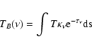$$% T_{B}(\nu)=\int{T \kappa_\nu \rm {e}^{-\tau_\nu} ds}$$ (1)

where $\kappa_\nu$ is the free-free absorption coefficient (given by Zirin 1988), $\tau_\nu=\int{\kappa_\nu {\rm d}s}$ is the optical depth, and T is the physical temperature of the medium. The integrals are performed along the line-of-sight.

	Figure 3: Brightness temperature of the solar disk center at various frequencies from 1.4 to 405 GHz represented by symbols. The solid curve shows the result obtained from our model.
Open with DEXTER

The hybrid model described above fits the brightness temperature of radio observations from 1.4 to 400 GHz very well as is shown in Fig. 3. As for 17 GHz, most of the emission arises from a region 2900 km above the solar surface, where  $\tau\sim 1$. In this region, the temperature is about 9600 K whereas the density (electrons and ions) is 9.3 $\times$ $10^9~{\rm cm}^{-3}$, yielding a brightness temperature of 10 390 K, which is very close to the value of 10⁴ K adopted by NoRH 17 GHz maps.

Once the atmospheric temperature and density profiles as a function of height have been established (see Table 1), two bi-dimensional matrices, representing one quadrant of the Sun, were created one for the temperature and another for the product of the electron and proton densities, $n_{\rm e} n_{\rm p}$, where each matrix pixel represents a square area of 50 $\times$ 50 km². In order to save computational time and memory due to the large number of empty pixels (e.g. regions below the solar surface) since we are only interested in the solar atmosphere, we divided the solar atmosphere into 7 smaller matrices both for the temperature and density product. These matrices follow the solar spherical curvature, as can be seen in Fig. 4. Since we have to follow the radiation path near the solar limb, the region covered by the matrices is slightly larger than one quadrant (90$^\circ$), in fact it ranges from polar angles $-10^\circ$ through $100^\circ$.

	Figure 4: Representation of the 2-D solar atmosphere showing the regions covered by the temperature and density matrices. In this picture, Earth direction is to the right, making disk center at $0^\circ$ and limb at the top, at $90^\circ$.
Open with DEXTER

In order to calculate the brightness temperature as a function of distance from disk center all the way to the limb, the opacity integral and that of Eq. (1) are estimated along the horizontal lines of the 7 matrices described above. We have computed the brightness temperature every 14 lines, which corresponds to a distance of 700 km (approximately 1''). This value was chosen based on the spatial resolution of the NoRH maps, which is of 10''. Nevertheless, we cannot increase the pixel size (50 km) of the matrices because of the transition region which is in reality very thin and would otherwise be suppressed from the simulation (that is, its width would be much smaller than on pixel).

	Figure 5: Center-to-limb variation of the brightness temperature at 17 GHz, obtained from the model described in the text. The solid line is the result of the convolution of the model results (crosses) with the 10'' Nobeyama synthesized beam.
Open with DEXTER

  
2.1 Comparison with 17 GHz limb observations

Figure 5 shows the results for the calculation of the brightness temperature from disk center to the limb. The result is folded at disk center in order to simulate the observations, that is, from one limb to the opposite one. From this simulation it is possible to measure the brightness temperature at disk center and at the limb, or in other words the temperature excess above disk center values, and also the radius of the Sun defined as the distance where the disk center intensity falls to half its value. These results are listed on Table 2.

As can be seen from the figure, a limb brightening of 100% (crosses) with respect to the values at disk center is obtained from the model. Since this result was obtained with a spatial resolution of 1'', and the NoRH observations have a resolution of 10'', we have convolved this result with a 10'' FWHM Gaussian beam. The result of this convolution is shown as a solid line in Fig. 5. The excess temperature at the limb now has decreased to 36% above disk center values.

Despite the good agreement at disk center, $T_B\sim 10^4$ K, the values at the limb are of the order of the maximum values measured at the polar limbs of NoRH maps (Selhorst et al. 2003) and much larger than those of 10-15% observed at equatorial limb regions (in the absence of active regions). The limb brightening width of 34'', that is the distance where the intensity is half the maximum value of the excess above quiet Sun, is also much smaller than that measured from 17 GHz maps, which is on average 66 $\pm$ 16 arcsec (Selhorst et al. 2003). As for the radius determined after the convolution, the measured value of 970'' from this simulation is at least 5'' smaller than the mean solar radius measured from 17 GHz maps (Selhorst et al. 2004). Before convolution, a radius of 966.5'' was measured, increasing the discrepancy with observations even more.

  
3 Inclusion of spicules in the 1-D model

As can be seen from the results of the model described in the previous section, a spherically symmetric homogeneous atmosphere is not a good representation of the 17 GHz observations. In order to obtain a model closer to reality, we decided to create an inhomogeneous atmosphere by including spicules. Observations of spicules, mainly in H$\alpha$, show them as elongated structures lasting from 5 to 15 min, and covering from 1 to 10% of the solar surface (Sterling 2000). Since spicules reach heights greater than 3000 km above the solar surface, they are present in the regions where the 17 GHz emission is produced.

In the model, spicules are represented as cylinders of constant density and temperature plasma with solar composition, inclined with respect to the solar surface. Here, it is assumed that at the location of the spicules, the atmospheric material is substituted by that of the spicule, that is, the density and temperature values of the matrices are replaced by those of the spicules. A further assumption is that the rest of the atmosphere is unaltered. As spicules are chromospheric structures commonly observed in H$\alpha$, we define the base of the spicules at 1000 km above the photosphere, following Braun & Lindsey (1987).

A first test of the spicules influence on the 17 GHz emission was to simulate the effect the total height reached by the spicule would cause in the brightness temperature measured at disk center. The results of the simulation are shown in Fig. 6. In each panel, the height reached by a spicule starts at 1000 km and increases up to a maximum value of 10 000 km, the curves represent spicule temperature varying between 7000 and 13 000 K, with a 1500 K step. Each panel shows the results for a constant density, which varies from panel to panel in steps of 10¹⁰ cm^-3, starting at 2 $\times$ 10¹⁰ cm^-3. The main results obtained from this test for the brightness temperature, T_B, measured at disk center are:

• for heights varying from 1000 up to approximately 2500 km, the brightness temperature is not altered since the spicules are completely below the region where the 17 GHz is formed (2900 km), thus the brightness is determined by the atmosphere;
• the largest variations occur when the height of the spicule reaches 2500 up to 3700 km ( $\tau\sim 1$). For larger heights, the brightness temperature barely alters, since the spicule material is optically thick and the area covered by the spicules basically does not increase at disk center;
• for the same density, T_B increases as the spicule temperature increases;
• the brightness temperature increases as the spicule density increases up to 4 $\times$ 10¹⁰ cm^-3, and decreases for larger density values.

	Figure 6: The plots show the effect of the brightness temperature measured at disk center as a function of the spicule height for different values of spicules temperature and density.
Open with DEXTER

The temperature and height values used in the characterization of spicules are the ones commonly found in the literature (Coates 1958; Beckers 1968 and 1972; Cheng 1992; Sterling 2000; Saito et al. 2001), however there are few estimates as to their density. For a spicule composed mainly of hydrogen, the density is 3-18 $\times$ 10¹⁰ cm^-3. The plots in Fig. 6 show that densities higher than 8 $\times$ 10¹⁰ cm^-3 would decrease the brightness temperature to very low values even for hot spicules, that would reduce the disk center brightness temperature and completely suppress the limb brightening.

   
4 Results of 2-D model with spicules

The 2-D model of the solar atmosphere with spicules was constructed by randomly distributing spicules within the temperature and density matrices (Fig. 7). The brightness temperature as function of distance from disk center was calculated in the same way as in the homogeneous atmosphere (Sect. 2). The total number of spicules included in the model was equivalent to 10% of the solar surface covered by spicules.

Initially, the simulations were performed with spicules of constant height, width, temperature, and density, except for their locations and inclination angle that were randomly attributed. Eventually, the other physical properties (height, width, temperature, and density) were also varied. An example of the spicule distribution over the solar atmosphere can be seen in Fig. 7.

	Figure 7: Distribution of spicules over the solar limb.
Open with DEXTER

The result of a single simulation is shown in Fig. 8, where the center-to-limb brightness temperature variation is depicted by crosses. The dispersion of the points reflects the presence or absence of a spicule crossing that particular line-of-sight. Depending on the physical characteristics of the spicule it may yield a brightness temperature higher or lower than the surrounding atmosphere. Many simulations with spicules of random parameters were performed, and the mean of the brightness temperature distribution was calculate in order to obtain the final center-to-limb brightness temperature, $T_{\rm b}(r)$, for the model. The mean  $T_{\rm b}(r)$ is shown in Fig. 9 (crosses), along with the result from the convolution with a 10'' beam representing the NoRH observations (solid line).

	Figure 8: Brightness temperature center-to-limb variation for a single simulation using the atmospheric model with spicules.
Open with DEXTER

	Figure 9: Center-to-limb brightness temperature distribution for a mean of 28 simulations using the atmospheric model with spicules (crosses). The solid line depicts the convolution of the brightness temperature with a 10'' Gaussian beam representing the NoRH spatial resolution.
Open with DEXTER

The total number of center-to-limb brightness temperature simulations, N, was determined by a convergence criterion in which the mean of N simulations is calculated; from which the rms of the 400 points closest to disk center is determined; this rms and that calculated from N+1 simulations should be less than 0.0003. Usually, it suffices to perform 20-40 simulations. In the following sections we present the results obtained from varying each of the spicule physical properties such as temperature, density, width, and height.

4.1 Effects of spicule parameter variation

The first line of Table 2 lists the results from the homogeneous model, i.e., from a spiculeless atmosphere. The next four lines of the table list the simulation results with spicules 500 km wide and 5000 km high, electron and ion density of 4 $\times$ 10¹⁰ cm^-3 and random inclination from 30 to 150$^\circ$with respect to the solar surface are shown in Fig. 10 and listed in Table 2. Each panel of the figure depicts the brightness temperature variation as function of disk center distance for different spicule temperatures, starting at 6000 K (Fig. 10a) and increasing by steps of 2000 K up to 12 000 K (Fig. 10d).

These results show that as the spicule temperature increases so do the quiet Sun brightness temperature and limb brightening, whereas the limb brightening width decreases.The solar radius measured at half quiet Sun value increases slightly with spicule temperature.

Before studying the effect of spicule density variation, the height of the spicule was chosen as a random value in the range of 5000 to 7000 km. The spicule electron and ion densities were considered to be equal. The results of varying the spicule density from 2 to 6 $\times$ 10¹⁰ cm^-3 are displayed in Table 2 and in Fig. 11. The simulations yield similar results to the 1-D model, i.e., that both the central disk brightness temperature and limb brightening increase with the spicule density up to 4 $\times$ 10¹⁰ cm^-3, and decreases thereafter. For the same temperature and density (10 000 K and 4 $\times$ 10¹⁰ cm^-3) as the previous simulation, the solar radius increased by 2'' indicating that the solar radius at 17 GHz reflects the average height reached by spicules.

Next, the effect of different spicule widths were analyzed. The spicule width is the only fixed parameter, starting at 500 km and increasing in steps of 200 km. In each simulation, spicule height varies randomly from 5000 to 7000 km, inclination from 30$^\circ$ to 150$^\circ$ as before, temperature from 7000 to 13 000 K, and density from 2 to 6 $\times$ 10¹⁰ cm^-3. Since the number of spicules was kept constant, an increase in their width implies that a larger area of the solar surface is covered. The results listed on Table 2 show very little variation in disk center brightness temperature (within the uncertainty), limb brightening (2%), and solar radius.

	Figure 10: Brightness temperature center-to-limb variation, mean from a set of simulations using the atmospheric model with spicules of different temperatures.
Open with DEXTER

	Figure 11: Brightness temperature center-to-limb variation, mean from a set of simulations using the atmospheric model with spicules of different densities.
Open with DEXTER

4.2 Influence of spicule height

A more detailed study of the influence of spicule height is performed, since there was an indication that the solar radius is sensitive to the average height of the spicules. New simulations were made, with all parameters, except the width, varying randomly. The only difference is that the upper limit to the spicule height increases by factors of 1000 km in each set of simulations.

In Fig. 12 and last lines of Table 2, the results show that neither the disk center brightness temperature nor the limb brightening are affected by the spicule height. These limb brightening values are compatible to what is observed in the equatorial and  $\pm45^\circ$ limb (Selhorst et al. 2003). The calculated solar radius values, however, reinforce our previous result that the 17 GHz radius increases as the spicule reaches higher in the chromosphere. These results agree with Horne et al. (1981) who proposed that spicules are optically thick at 235 GHz, and are responsible for the increase in the apparent radius of the Sun. Moreover, eclipse observation (Belkora et al. 1992) showed a very good correspondence between the extension of the solar limb at 3 mm and the height of H$\alpha$ spicules.

	Figure 12: Solar radius dependence on average spicule height, h.
Open with DEXTER

4.3 Comparison with 17 GHz observations

A comparison with observations is shown in Fig. 13, as a gray line whereas the model is depicted as the solid black line. The observation is a scan through the solar equator of a 17 GHz solar map taken during the last solar minimum, when there were no active regions near the equatorial limb. The intensity, or brightness temperature, is normalized to the quiet Sun value taken as the most common value of the map. The model result plotted on this figure was obtained by varying randomly all physical parameters of the spicules (except the width which is kept at 500 km): temperatures of 7000-13 000 K, densities in the range 2-6 $\times$ 10¹⁰ cm^-3, inclination angle between  $30^\circ{-}150^\circ$, and heights of 5000 to 7000 km. The agreement of the model with the data is remarkable, reproducing very well the 12% limb brightening and its width observed in the solar map of this day.

	Figure 13: Comparison between the observational profile at the equator (gray) and the mean of the simulations (black).
Open with DEXTER

  
5 Discussion and conclusions

A model for the solar atmosphere, from the photosphere all the way to the corona, was constructed taking into account three observational radio data: (i) brightness temperature of quiet Sun (1.4-400 GHz); (ii) limb brightening (17 GHz); and (iii) solar radius at half the quiet Sun value (17 GHz). The model presented here is based on previous models for the photosphere (Fontenla et al. 1993), chromosphere (Zirin 1988; Zirin et al. 1991), and corona (Gabriel 1992).

The first model was spherically symmetric, without any structures such as spicules, and is described by temperature and density matrices which values are given in Table 1. In this model, the transition region occurs at 3500 km above the solar surface and is about 100 km wide. This transition region is about 1000 km higher than that typically used in the VAL and FAL models. The VAL C model locates the transition region at approximately 2300 km above the photosphere. This discrepancy may be due to underestimated abundances of metals used in the UV line calculation (Zhang et al. 2001).

The model presented here may be seen as a representation of the dynamic nature of the chromosphere (Carlsson & Stein 1995), where each individual simulation represents a snapshot of the time-variable atmosphere. The authors show that the temperature enhancement at 2000 km proposed by the FAL model is not real and may be produced by temporally varying waves, while the effective temperature of the chromosphere below 1800 km is still decreasing. We point out that our model is not in disagreement with the temperature distribution proposed by Carlsson & Stein (1995). First, our model locates the transition region at 3500 km, and not at around 2000 km as in the FAL model, and second, the region below 2000 km is optically thick to the 17 GHz emission. In order to test the decreasing temperature distribution set forth by Carlsson & Stein (1995), observations at higher frequencies are needed. This will be investigated in a future work.

The brightness temperature as a function of distance from disk center was calculated by integrating along parallel paths. The main results from this model were:

• Very good agreement with the quiet Sun brightness temperatures reported in the literature at several frequencies from 1 to 400 GHz. At 17 GHz, $T_{\rm b}=10~392$ K that is compatible with the quoted value of 10⁴ K.

• A limb brightening of 36% above quiet Sun values, after convolution with a 10'' FWHM Gaussian representing the synthesized beam of NoRH. This result resembles that of the solar poles, however, it is somewhat larger than the brightening observed at equatorial ($\sim$15%) and intermediate ($\sim$10%) regions (see Selhorst et al. 2003).

• The solar radius obtained from the model was ($\sim$970''), which is at least 5'' smaller than the mean observed value (Selhorst et al. 2004).

Since the limb brightening was too large, we decided to introduce spicules in our model. Several authors have claimed that spicules were responsible for a decrease in the limb brightening of radio observations, especially at microwaves (Elzner 1976; Fürst et al. 1974; Braun & Lindsey 1987). Spicules were modeled as cylindrical structures of constant density (electron equals ion density) and temperature, starting at 1000 km from the solar photosphere and inclined with respect to it. It was assumed that at any given time, 10% of the solar surface was covered by spicules. The physical characteristics of each spicule (such as density, temperature, height, and inclination angle) were attributed randomly. The spicule width was kept at a constant value of 500 km in the simulations.

The center-to-limb brightness temperature distribution was determined in the same was as in the first model, and the results showed that:

• The quiet Sun brightness temperature and limb brightening increase as the temperature of the spicule increases.

• The quiet Sun brightness temperature and limb brightening increase with density up to 4 $\times$ 10¹⁰ cm^-3, and decreases for higher spicule density values.

• The solar radius at 17 GHz is determined by the average height of the spicules, increasing as the height increases.

• Limb brightening values of 12% are obtained by varying randomly the physical parameters of spicules. This limb brightness temperature increase agrees with observations at 17 GHz, except for the polar regions.

In conclusion, the atmospheric model, from the photosphere to the coronal levels, presented here is able to reproduce well the quiet Sun brightness temperature at disk center from 1 to 400 GHz, the measured radius at 17 GHz, and the limb brightening observed in NoRH solar maps, except the polar regions which will be discussed elsewhere (Selhorst et al. 2005). Nevertheless, in order to reproduce the observations at radio wavelengths, it was necessary to include absorbing chromospheric structures such as spicules. The spicules parameters had random values in the range commonly found in the literature. As a final note, we point out that this model should also be able to reproduce the photospheric line observations since our model uses the values from Fontenla et al. (1993) model.

Acknowledgements

C.L.S. acknowledges support from the Brazilian agency FAPESP, grant number 01/02106-3. The Nobeyama Radioheliograph is operated by NAOJ/Nobeyama Solar Radio Observatory.

References

• Beckers, J. M. 1968, Sol. Phys., 3, 367 [NASA ADS] (In the text)
• Beckers, J. M. 1972, ARA&A, 10, 73 [NASA ADS] (In the text)
• Beckman, J. E., Clark, C. D., & Ross, J. 1973, Sol. Phys., 31, 319 [NASA ADS] [CrossRef]
• Belkora, L., Hurford, G. J., Gary, D. E., & Woody, D. P. 1992, ApJ, 400, 692 [NASA ADS] [CrossRef] (In the text)
• Braun, D., & Lindsey, C. 1987, ApJ, 320, 898 [NASA ADS] [CrossRef] (In the text)
• Carlsson, M., & Stein, R. F. 1995, ApJ, 440, L29 [CrossRef] (In the text)
• Cheng, Q. 1992, A&A, 266, 537 [NASA ADS] (In the text)
• Coates, R. J. 1958, ApJ, 128, 83 [NASA ADS] [CrossRef] (In the text)
• Elzner, L. R. 1976, A&A, 47, 9 [NASA ADS] (In the text)
• Ewell, M. W., Zirin, H., Jensen, J. B., & Bastian, T. S. 1993, ApJ, 403, 426 [NASA ADS] [CrossRef] (In the text)
• Fontenla, J. M., Avrett, E. H., & Loeser, R. 1990, ApJ, 355, 700 [NASA ADS] [CrossRef] (In the text)
• Fontenla, J. M., Avrett, E. H., & Loeser, R. 1991, ApJ, 377, 712 [NASA ADS] [CrossRef] (In the text)
• Fontenla, J. M., Avrett, E. H., & Loeser, R. 1993, ApJ, 406, 319 [NASA ADS] [CrossRef] (In the text)
• Fürst, E., Hachenberg, O., & Hirth, W. 1974, A&A, 36, 123 [NASA ADS] (In the text)
• Gabriel, A. H. 1992, in The Sun, A Laboratory for Astrophysics, ed. J. T. Schmelz, & J. C. Brown (Kluwer Academic Publishers), 277 (In the text)
• Gingerich, O., Noyes, R. W., Kalkofen, W., & Cuny, Y. 1971, Sol. Phys., 18, 347 [NASA ADS] [CrossRef] (In the text)
• Horne, K., Hurord, G. J., Zirin, H., & de Graauw, Th. 1981, ApJ, 244, 340 [NASA ADS] [CrossRef] (In the text)
• Kuseski, R. A., & Swanson, P. N. 1976, Sol. Phys., 48, 41 [NASA ADS] [CrossRef]
• Linsky, J. L. 1973, Sol. Phys., 28, 409 [NASA ADS] [CrossRef]
• Roellig, T. L., Becklin, E. E., Jefferies, J. T., et al. 1991, ApJ, 381, 288 [NASA ADS] [CrossRef] (In the text)
• Saito, T., Kudoh, T., & Shibata, K. 2001, ApJ, 554, 1151 [NASA ADS] [CrossRef] (In the text)
• Selhorst, C. L., Silva, A. V. R., Costa, J. E. R., & Shibasaki 2003, A&A, 401, 1143 [EDP Sciences] [NASA ADS] [CrossRef] (In the text)
• Selhorst, C. L., Silva, A. V. R., & Costa, J. E. R. 2004, A&A, 420, 1117 [EDP Sciences] [NASA ADS] [CrossRef] (In the text)
• Selhorst, C. L., Silva, A. V. R., & Costa, J. E. R. 2005, in preparation (In the text)
• Shibasaki, K. 1998, in Synoptic Solar Physics, ed. K. S. Balasubramaniam, J. Harvey, & D. Rabin, ASP Conf. Ser., 140, 373 (In the text)
• Sterling, A. C. 2000, Sol. Phys., 196, 79 [NASA ADS] [CrossRef] (In the text)
• Vernazza, J. E., Avrett, E. H., & Loeser, R. 1973, ApJ, 184, 605 [NASA ADS] [CrossRef] (In the text)
• Vernazza, J. E., Avrett, E. H., & Loeser, R. 1976, ApJS, 30, 1 [NASA ADS] [CrossRef] (In the text)
• Vernazza, J. E., Avrett, E. H., & Loeser, R. 1981, ApJS, 45, 635 [NASA ADS] [CrossRef] (In the text)
• Zhang, J., Kundu, M. R., White, S. M., Dere, K. P., & Newmark, J. S. 2001, ApJ, 561, 396 [NASA ADS] [CrossRef] (In the text)
• Zirin, H. 1988, in Astrophysics of the Sun (New York, Cambridge: Cambridge University Press) (In the text)
• Zirin, H., Baumert, B. M., & Hurford, G. J. 1991, ApJ, 370, 779 [NASA ADS] [CrossRef] (In the text)