A&A 432, 921-935 (2005)
DOI: 10.1051/0004-6361:20041810
F. Fontani 1 - M. T. Beltrán 2 - J. Brand 3 - R. Cesaroni 2 - L. Testi 2 - S. Molinari 4 - C. M. Walmsley 2
1 - Dipartimento di Astronomia e Fisica dello spazio, Largo E. Fermi 2,
50125 Firenze, Italy
2 -
INAF, Osservatorio Astrofisico di Arcetri, Largo E. Fermi 5,
50125 Firenze, Italy
3 -
Istituto di Radioastronomia, CNR, via Gobetti 101, 40129 Bologna,
Italy
4 -
IFSI, CNR, via Fosso del Cavaliere, 00133 Roma, Italy
Received 6 August 2004 / Accepted 15 November 2004
Abstract
We have observed two rotational transitions of both CS
and C17O, and the 1.2 mm continuum emission towards
a sample of 130 high-mass protostellar candidates with ![]() <
<
![]() .
This work represents the first step of the extension to the southern
hemisphere of a project started more than a decade ago aimed at the
identification of massive protostellar candidates.
Following the same approach adopted for sources with
.
This work represents the first step of the extension to the southern
hemisphere of a project started more than a decade ago aimed at the
identification of massive protostellar candidates.
Following the same approach adopted for sources with
![]()
![]()
![]() ,
we have selected from the IRAS Point Source
Catalogue 429 sources which potentially are compact molecular clouds
on the basis of their IR colours. The sample has then been divided into two groups according to the colour indices [25-12] and [60-12]: the
298 sources with [25-12]
,
we have selected from the IRAS Point Source
Catalogue 429 sources which potentially are compact molecular clouds
on the basis of their IR colours. The sample has then been divided into two groups according to the colour indices [25-12] and [60-12]: the
298 sources with [25-12] ![]() 0.57 and [60-12]
0.57 and [60-12] ![]() 1.30 have been
called High sources, the remaining 131 have been called
Low sources. In this paper, we check the association
with dense gas and dust in 130 Low sources. We have obtained
a detection rate of
1.30 have been
called High sources, the remaining 131 have been called
Low sources. In this paper, we check the association
with dense gas and dust in 130 Low sources. We have obtained
a detection rate of ![]()
![]() in CS, demonstrating a tight
association of the sources with dense molecular clumps.
Among the sources detected in CS,
in CS, demonstrating a tight
association of the sources with dense molecular clumps.
Among the sources detected in CS,
![]()
![]() have also been detected in C17O and
have also been detected in C17O and ![]()
![]() in the 1.2 mm continuum.
Millimeter-continuum maps show the presence of clumps with diameters
in the range 0.2-2 pc and masses from a few
in the 1.2 mm continuum.
Millimeter-continuum maps show the presence of clumps with diameters
in the range 0.2-2 pc and masses from a few ![]() to
to
![]() ;
H2 volume densities
computed from CS line ratios lie between
;
H2 volume densities
computed from CS line ratios lie between ![]() 104.5 and 105.5 cm-3.
The bolometric luminosities of the sources, derived from IRAS data, are in the
range
104.5 and 105.5 cm-3.
The bolometric luminosities of the sources, derived from IRAS data, are in the
range
![]() ,
consistent with embedded high-mass objects.
Based on our results
and those found in the literature for other samples
of high-mass young stellar objects, we conclude that our sources are
massive objects in a very early evolutionary stage, probably
prior to the formation of an H II region. We
propose a scenario in which High and Low sources are
both made of a massive clump hosting a high-mass protostellar
candidate and a nearby stellar cluster. The difference might be due
to the fact that the 12
,
consistent with embedded high-mass objects.
Based on our results
and those found in the literature for other samples
of high-mass young stellar objects, we conclude that our sources are
massive objects in a very early evolutionary stage, probably
prior to the formation of an H II region. We
propose a scenario in which High and Low sources are
both made of a massive clump hosting a high-mass protostellar
candidate and a nearby stellar cluster. The difference might be due
to the fact that the 12 ![]() m
IRAS flux, the best discriminant between the two groups, is dominated by
the emission from the cluster in Lows and from the massive
protostellar object in Highs.
m
IRAS flux, the best discriminant between the two groups, is dominated by
the emission from the cluster in Lows and from the massive
protostellar object in Highs.
Key words: stars: formation - radio lines: ISM - ISM: molecules
Recently, an ever growing effort has been devoted to investigating
the early evolutionary stages of massive stars (
![]() ).
In particular, attention has gradually shifted from the study of newly
formed ZAMS stars to
objects in an earlier evolutionary stage, prior to the formation of
an H II region, deriving their luminosity from the release of
gravitational energy: these objects are named protostars.
The observational approach to searching for high-mass protostars was first
formulated by Habing &
Israel (1979): likely candidates must be associated
with dense circumstellar environments, not be associated with HII regions,
and they should have high luminosities.
).
In particular, attention has gradually shifted from the study of newly
formed ZAMS stars to
objects in an earlier evolutionary stage, prior to the formation of
an H II region, deriving their luminosity from the release of
gravitational energy: these objects are named protostars.
The observational approach to searching for high-mass protostars was first
formulated by Habing &
Israel (1979): likely candidates must be associated
with dense circumstellar environments, not be associated with HII regions,
and they should have high luminosities.
Following these criteria, with the aim of identifying massive protostellar
candidates (with
![]() ),
Palla et al. (1991) selected a
sample of 260 sources from the IRAS Point Source Catalogue (IRAS-PSC)
with 60
),
Palla et al. (1991) selected a
sample of 260 sources from the IRAS Point Source Catalogue (IRAS-PSC)
with 60 ![]() m flux greater than 100 Jy and colours satisfying the
criteria established by Richards et al. (1987) for
compact molecular cores. This sample was then divided into two groups
according to their [25-12] and [60-12] colours: the High sources,
which have [25-12]
m flux greater than 100 Jy and colours satisfying the
criteria established by Richards et al. (1987) for
compact molecular cores. This sample was then divided into two groups
according to their [25-12] and [60-12] colours: the High sources,
which have [25-12] ![]() 0.57 and [60-12]
0.57 and [60-12] ![]() 1.30 characteristic of association with UC H II regions (Wood & Churchwell 1989), and
the Low sources, with complementary colours. Palla et al.
found a lower association
rate with H2O masers for the Low sources, and interpreted
this as an indication of relative youth.
In order to confirm this result, and to better understand the nature of
High and Low sources, the whole sample has been studied in various
tracers, including
molecular lines and continuum emission, from centimeter to near-infrared
wavelengths (Molinari et al. 1996, 1998a, 2000,
2002; Brand et al. 2001; Zhang et al. 2001). The main findings of these studies are the following:
1.30 characteristic of association with UC H II regions (Wood & Churchwell 1989), and
the Low sources, with complementary colours. Palla et al.
found a lower association
rate with H2O masers for the Low sources, and interpreted
this as an indication of relative youth.
In order to confirm this result, and to better understand the nature of
High and Low sources, the whole sample has been studied in various
tracers, including
molecular lines and continuum emission, from centimeter to near-infrared
wavelengths (Molinari et al. 1996, 1998a, 2000,
2002; Brand et al. 2001; Zhang et al. 2001). The main findings of these studies are the following:
The results obtained for sources with
![]() suggested an extension to sources with
suggested an extension to sources with
![]() following the same approach, in order to complete this study.
With this motivation, we have applied
the selection criteria of Palla et al. (1991) to
sources of the IRAS-PSC with
following the same approach, in order to complete this study.
With this motivation, we have applied
the selection criteria of Palla et al. (1991) to
sources of the IRAS-PSC with
![]() ,
finding
298 High and 131 Low sources. It is worth noting that
the samples selected by us likely contain a higher contamination
of H II regions than those selected by
Palla et al. (1991), because surveys of H II regions south of
,
finding
298 High and 131 Low sources. It is worth noting that
the samples selected by us likely contain a higher contamination
of H II regions than those selected by
Palla et al. (1991), because surveys of H II regions south of
![]() are much less numerous than those
with
are much less numerous than those
with
![]() .
.
When identifying massive protostellar candidates, the first step is to establish an association with dense molecular clumps. Dense gas is traced by warm dust emission from a massive core at millimeter and sub-millimeter wavelengths, and by millimeter rotational and inversion transitions of various molecular species, such as CS, NH3 and C17O. In this paper we present observations obtained with the SEST-15 m telescope of rotational transitions of CS and C17O, and of the 1.2 mm continuum emission towards almost all (130 out of 131) sources belonging to the Low subsample.
All sources belonging to the High subsample have already been observed in the CS (2-1) line by Bronfman et al. (1996), who performed a complete survey in this line towards IRAS sources with [25-12] and [60-12] colours characteristic of UC H II regions with the SEST and the Onsala telescope.
Also, an alternative sample of high-mass protostellar candidates has been selected from the IRAS-PSC by Sridharan et al. (2002). They used selection criteria similar to those of Palla et al. (1991), with the important difference that they ruled out all Low sources, and therefore their sample is basically made of High sources. Then, Beuther et al. (2002a) observed the molecular environment associated with these sources in some CS lines and 1.2 mm continuum. Therefore, their results, as well as those of Bronfman et al. (1996), are of great interest for the present paper, and will be used in the following for the sake of comparison to our findings. Hereafter, the sample selected by Sridharan et al. (2002) and observed in various tracers by Beuther et al. (2002a) will be called "Sridharan/Beuther sample''. All the sources detected in the CS (2-1) line by Bronfman et al. (1996) have been observed by Faundez et al. (2004) in the 1.2 mm continuum. However, we have not used their results in this paper because their work was published after our paper was submitted. They will be discussed in a forthcoming paper (Beltran et al., in prep.) entirely devoted to the observations of the millimeter continuum (see Sect. 3.3).
Section 2 describes the observations, and Sect. 3 presents the results. In Sect. 4 we derive the physical properties of the molecular clumps, which we discuss in Sect. 5. The conclusions are summarized in Sect. 6.
Single-pointing observations of CS and C17O were obtained with the SEST (Swedish-ESO Submillimetre Telescope) 15-m telescope at ESO-La Silla, Chile. In Table 1 we give the molecular transitions observed (Col. 1), the line rest frequencies (Col. 2), the telescope half-power beam width (HPBW, Col. 3), and the channel spacing (Col. 4) and total bandwidth (Col. 5) of the spectrometer used.
All observations were carried out towards the positions of the
IRAS sources given in Table A.1. We observed using
dual beam switching
with a
![]()
![]() throw. The data were calibrated with the chopper
wheel technique (see Kutner & Ulich 1981). Pointing was checked
every 1-2 h on SiO masers at 7 mm. The pointing accuracy is
estimated to be
throw. The data were calibrated with the chopper
wheel technique (see Kutner & Ulich 1981). Pointing was checked
every 1-2 h on SiO masers at 7 mm. The pointing accuracy is
estimated to be ![]() 3
3
![]() .
.
Table 1: Observed transitions.
Observations of the CS (2-1), (3-2) and (5-4) lines were performed
from May 23 to 25, 2001, and from May 6 to 11, 2002.
We observed the (2-1), (3-2) and (5-4) lines respectively
in 130, 128 and 3 out of 131 sources of the initial sample.
The antenna temperature,
![]() and the main beam
brightness temperature
and the main beam
brightness temperature
![]() are related as:
are related as:
![]() ,
with
,
with
![]() ,
0.66 and 0.50 for CS (2-1), (3-2) and (5-4) respectively.
,
0.66 and 0.50 for CS (2-1), (3-2) and (5-4) respectively.
We simultaneously observed the (2-1) and (3-2) lines during the first
observing run, and the (2-1) and (5-4) lines during the second observing
run, using two Acusto-Optic Spectrometers: one with low spectral
resolution and large bandwidth, and a second with higher
spectral resolution and smaller bandwidth (see Table 1).
Since the
![]() was unknown for most sources we tuned the receivers to the
was unknown for most sources we tuned the receivers to the
![]() of the tangent point for the source galactic longitude
(see Table A.1).
The values of
of the tangent point for the source galactic longitude
(see Table A.1).
The values of
![]() used during the first and the second observing
runs are listed in Cols. 4 and 5, respectively.
The integration time ranged from 3 to 4.5 min.
For some lines detected at the edge of the bandwidth in the first scan
we integrated the minimum possible time to get
a low S/N detection of the CS (2-1) line in low resolution; after having
determined the
used during the first and the second observing
runs are listed in Cols. 4 and 5, respectively.
The integration time ranged from 3 to 4.5 min.
For some lines detected at the edge of the bandwidth in the first scan
we integrated the minimum possible time to get
a low S/N detection of the CS (2-1) line in low resolution; after having
determined the
![]() of the line, we then re-centered the high
resolution backend and made another measurement.
of the line, we then re-centered the high
resolution backend and made another measurement.
For 5 sources (13558-6159, 15262-5541, 16170-5053, 16402-4943, 16581-4212) observed during the first run we obtained bad quality spectra. We thus repeated the observations in the second run.
C17O (1-0) and (2-1) lines were observed in the period from
May 6 to 11, 2002. For sources previously detected in CS we have
used the LSR velocity of these lines to center the backends.
We have also observed 8 objects not detected in CS.
For these, we used the same velocity adopted for the CS observations,
computed as described in Sect. 2.1.1.
We observed the (1-0) and (2-1)
transitions simultaneously using the 3 and 1.3 mm receivers.
As for the CS lines,
![]() and
and
![]() are related as
are related as
![]() ,
with
,
with
![]() and 0.50
for the C17O(1-0) and (2-1) lines, respectively.
and 0.50
for the C17O(1-0) and (2-1) lines, respectively.
The C17O (1-0) and (2-1) rotational transitions have hyperfine structure (see e.g. Frerking & Langer 1981). To take this into account, we fitted the lines using METHOD HFS of the CLASS program, which is part of the GAG-software developed at the IRAM and the Observatoire de Grenoble. This fits the lines assuming that all components have equal excitation temperatures, that the line separations are fixed at the laboratory values, and that the line widths are identical. This method also gives an estimate of the total optical depth of the lines based on the intensity ratio of the different hyperfine components.
The 1.2 mm continuum observations were carried out with the 37-channel bolometer array SIMBA (SEST Imaging Bolometer Array) at the SEST, on July 16-20, 2002 and July 9-13, 2003.
Maps were obtained towards all sources detected in CS, with
the exception of 10555-5949, and towards 12 sources undetected in CS.
Around all IRAS sources, we mapped a region of size 900
![]()
![]() 400
400
![]() (azimuth
(azimuth ![]() elevation), which was scanned at a rate of 80
elevation), which was scanned at a rate of 80
![]() /s.
The total integration time per map was about 15 min, and
the typical noise level in the maps is 25-40 mJy/beam.
Atmospheric opacity was determined from skydips, which were taken every 2 h, and values at the zenith ranged between 0.21 and 0.50 (in 2002) and
0.13 and 0.30 (2003). The data were calibrated using observations of
Uranus, made once or twice per day; the conversion factor ranged between 58 and 75 mJy/count in 2002, and between 50 and 69 in 2003.
The pointing of the SEST was determined to be accurate
within a few arcsec, by observing a strong continuum source every 2 h.
The HPBW is
/s.
The total integration time per map was about 15 min, and
the typical noise level in the maps is 25-40 mJy/beam.
Atmospheric opacity was determined from skydips, which were taken every 2 h, and values at the zenith ranged between 0.21 and 0.50 (in 2002) and
0.13 and 0.30 (2003). The data were calibrated using observations of
Uranus, made once or twice per day; the conversion factor ranged between 58 and 75 mJy/count in 2002, and between 50 and 69 in 2003.
The pointing of the SEST was determined to be accurate
within a few arcsec, by observing a strong continuum source every 2 h.
The HPBW is ![]() 24
24
![]() .
.
All data were reduced with the program MOPSI, written by R. Zylka
(Grenoble), and according to the instructions given in the SIMBA Observers
Handbook![]() (2003).
(2003).
The observed sources are listed in Table A.1. Column 1 gives the IRAS name,
and the equatorial (J2000) coordinates of the IRAS source
are listed in Cols. 2 and 3, respectively.
In Cols. 4 and 5 we list the center velocities used for the
CS observations during the first and the second
run, respectively, chosen as explained in Sect. 2.1.1.
In Cols. 6 to 8 we present the following information: detection (Y) or
non-detection (N) in CS, C17O and 1.2 mm continuum,
respectively (N.O. means "not observed''). For the millimeter continuum,
we have considered as detected those sources which show emission
above the 3![]() level in the maps.
In Col. 9 we give the angular separation,
level in the maps.
In Col. 9 we give the angular separation, ![]() ,
between the IRAS source and the peak position of the millimeter continuum. For sources with multiple peaks (see Sect. 3.3),
,
between the IRAS source and the peak position of the millimeter continuum. For sources with multiple peaks (see Sect. 3.3), ![]() represents the separation between the IRAS position and the nearest peak.
represents the separation between the IRAS position and the nearest peak.
In Table A.2 we list the CS line parameters obtained from the
high resolution spectra. Almost all observed lines are
well fitted by Gaussians, and the parameters
have been calculated from these fits, except where specified otherwise
(see discussion below). The integrated intensities,
![]() ,
of the CS (2-1) and (3-2) lines are given
in Cols. 2 and 5, respectively;
the line peak velocities,
,
of the CS (2-1) and (3-2) lines are given
in Cols. 2 and 5, respectively;
the line peak velocities,
![]() ,
are
listed in Cols. 3 and 6, and Cols. 4 and 7 list the line
widths at half maximum, FWHM. In Cols. 2 and 5 we also give
the
,
are
listed in Cols. 3 and 6, and Cols. 4 and 7 list the line
widths at half maximum, FWHM. In Cols. 2 and 5 we also give
the ![]() level, in K km s-1, of the spectra for non-detected sources,
obtained assuming an average value of FWHM = 2.5 km s-1.
level, in K km s-1, of the spectra for non-detected sources,
obtained assuming an average value of FWHM = 2.5 km s-1.
Several spectra show multiple velocity components (16187-4932, 16254-4844, 16344-4605, 16363-4645, 16535-4300, 17036-4033, 17225-3426, 17256-3631, 17285-3346, 17355-3241). For these sources, we have performed, where possible, Gaussian fits to all components (the corresponding Gaussian parameters are listed in Table A.2). The two components detected in 16535-4300 have also been detected in the C17O lines, whereas for 16363-4645 none of them were detected in C17O. For all other sources with multiple components, only one component has also been detected in C17O. In Sect. 4, where we will derive the physical properties of the clumps, we will refer to the CS component which has also been revealed in C17O; for 16363-4645 and 16535-4300 we have chosen the strongest one.
There are cases also in which the line profiles are asymmetric or
deviate significantly from a Gaussian shape.
In some spectra the lines have two blended peaks
(e.g. 10123-5727, 17040-3959 and 17377-3109). This could be due to the
superposition of separate velocity components,
or to self-absorption. Also, a few lines present broad wings
(e.g. 13438-6203, 15579-5303, 16218-4931, and 16204-4916).
Incidentally, we note that
15579-5303 and 16204-4916 have FWHM very much higher
than all other lines (![]() 10-11 km s-1).
For these lines, the
parameters listed in Table A.2 have been derived from moment
integrals over the velocity intervals indicated in parentheses in
Cols. 3 and 7.
10-11 km s-1).
For these lines, the
parameters listed in Table A.2 have been derived from moment
integrals over the velocity intervals indicated in parentheses in
Cols. 3 and 7.
We observed the C17O (1-0) and (2-1) lines towards all of the 111 sources detected in CS, and towards 8 sources not detected in CS. Emission was detected in 84 sources, all of them previously detected in CS (see Table 2): the C17O detection rate is thus ![]()
![]() for sources detected in CS,
and
for sources detected in CS,
and ![]()
![]() for all observed sources.
In Table A.3 we give the line parameters obtained from the high
resolution spectra: in Cols. 3-6 we list integrated
intensity (
for all observed sources.
In Table A.3 we give the line parameters obtained from the high
resolution spectra: in Cols. 3-6 we list integrated
intensity (
![]() ), peak velocity (
), peak velocity (
![]() ), FWHM
and opacity (
), FWHM
and opacity (![]() )
of the
C17O (1-0) line, respectively.
Columns 8-11 show the same parameters for the C17O (2-1) line.
The integrated intensities have been computed from integrals over the
velocity ranges given in Cols. 2 and 7 of Table A.3, while for the
other parameters we have adopted the fitting procedure
described in Sect. 2.1.3.
)
of the
C17O (1-0) line, respectively.
Columns 8-11 show the same parameters for the C17O (2-1) line.
The integrated intensities have been computed from integrals over the
velocity ranges given in Cols. 2 and 7 of Table A.3, while for the
other parameters we have adopted the fitting procedure
described in Sect. 2.1.3.
In several spectra the different hyperfine components are fairly well-resolved. Two examples are shown in Fig. 1, where we have also indicated the position of the hyperfine components. Only one source, 16535-4300, presents a secondary fainter velocity component as in the corresponding CS spectra. The optical depths show that the C17O (1-0) and (2-1) lines are optically thin in almost all detected sources. Therefore, in Sect. 4.1.2 we will assume optically thin conditions when computing kinetic temperatures and column densities of the molecule.
Table 2: Number of sources detected (Y), not detected (N) or not observed (N.O.) in C17O and 1.2 mm continuum among the 111 sources detected in CS.
![\begin{figure}
\par\includegraphics[width=8cm,clip]{1810fig1.ps}\end{figure}](/articles/aa/full/2005/12/aa1810/img68.gif) |
Figure 1: Spectra of the C17O (1-0) and (2-1) lines obtained towards 08563-4225 (top panels) and 15072-5855 (bottom panels). Vertical lines under the spectra indicate the hyperfine components. |
| Open with DEXTER | |
We mapped 124 sources in the 1.2 mm continuum, among which 109 out of the 111 sources detected in CS, and a further 15 sources not detected in CS. Since the present paper is focused on the molecular emission, hereafter we will discuss only the maps of the sources detected in CS. The analysis of the 1.2 mm continuum maps of all observed sources will be available in a forthcoming paper (Beltran et al., in prep.) completely devoted to this purpose. In that work, we will also compare our data with those of Faundez et al. (2004), who observed the 1.2 mm continuum emission towards a sample of High sources.
The observations show the presence of dusty clumps in 101 out of
109 sources previously detected in CS (see Table 2),
which translates into a detection rate of ![]()
![]() .
Morphologically, the maps show a large variety of features and structures.
In several cases we detected an isolated clump, but only a small
fraction of the clumps show a simple
spherical symmetry (e.g. 17040-3959). Most of them have an
elongated shape (e.g. 15557-5337), secondary faint peaks
(e.g. 16535-4300) or a core-halo structure
(e.g. 13481-6124). Additionally, the majority of the maps shows
multiple clumps. One can distinguish between sources in which the clumps
are separable (i.e. with the contours at half of the maximum well
separated),
and sources in which they are superimposed and not separable.
In Fig. 2 we show an example of an isolated spherical clump,
17040-3959, and two examples of "clumpy'' sources: in 10123-5727 the
clumps are separable, while in 17225-3426 they are not.
.
Morphologically, the maps show a large variety of features and structures.
In several cases we detected an isolated clump, but only a small
fraction of the clumps show a simple
spherical symmetry (e.g. 17040-3959). Most of them have an
elongated shape (e.g. 15557-5337), secondary faint peaks
(e.g. 16535-4300) or a core-halo structure
(e.g. 13481-6124). Additionally, the majority of the maps shows
multiple clumps. One can distinguish between sources in which the clumps
are separable (i.e. with the contours at half of the maximum well
separated),
and sources in which they are superimposed and not separable.
In Fig. 2 we show an example of an isolated spherical clump,
17040-3959, and two examples of "clumpy'' sources: in 10123-5727 the
clumps are separable, while in 17225-3426 they are not.
As already said, a detailed analysis of these maps will be provided in a forthcoming paper. For the present discussion, we concentrate only on the continuum source associated with the line emission. Some physical parameters of the clumps, derived from the molecular line data in Sect. 4, require an estimate of the source angular diameter. Since we have not made maps in the molecular lines, this estimate has been obtained from the continuum maps, making the assumption that the millimeter continuum and the molecular lines trace the same region. Although some authors have shown that in clumps associated with high-mass YSOs dust and molecular line emission may have different distribution (e.g. Fontani et al. 2004b), typically the angular diameters of their emitting regions are comparable. Thus, the assumption that the millimeter continuum and the molecular lines trace the same region is a reasonable approximation.
The lines were observed towards the position of the IRAS source;
we have thus searched for the continuum source which is closest to the
IRAS position.
For sources with multiple clumps we have assumed that the
IRAS source is associated with a particular
continuum clump if the IRAS source lies within the clump's 3![]() contour level.
For sources in which none of the clumps includes the IRAS position,
we have not assigned any "continuum source''.
contour level.
For sources in which none of the clumps includes the IRAS position,
we have not assigned any "continuum source''.
![\begin{figure}
\par\includegraphics[width=7cm,clip]{1810fig2.ps}\end{figure}](/articles/aa/full/2005/12/aa1810/img69.gif) |
Figure 2:
Examples of various morphologies of the 1.2 mm continuum
emission. a) 1.2 mm continuum map of 17040-3959. Contour levels range from 0.09 ( |
| Open with DEXTER | |
Finally, several sources require a comment:
The main physical properties of the sources are presented in three tables: the parameters that do not depend on the source distance are listed in Table A.4; in Table A.5 we give distances, source linear diameters and luminosities, and in Table A.6 we list the mass estimates. We now outline the methods used to derive each parameter, and present the results obtained.
The physical parameters which do not depend on the source distance are listed in Table A.4: the angular diameter of the clumps (Col. 2), the 1.2 mm continuum flux densities (Col. 3), the kinetic temperature, the C17O column density and the H2 total column density of the gas derived from the C17O lines (Cols. 4-6, respectively) and the H2 volume density obtained from the CS data (Col. 7).
The angular diameters (![]() )
of the clumps identified
in the 1.2 mm continuum maps (see Sect. 3.3)
have been computed assuming the sources are Gaussian, and
deconvolving the observed contour at half maximum with
a Gaussian beam of 24
)
of the clumps identified
in the 1.2 mm continuum maps (see Sect. 3.3)
have been computed assuming the sources are Gaussian, and
deconvolving the observed contour at half maximum with
a Gaussian beam of 24
![]() .
No angular diameter has been
attributed to those sources for which the IRAS position does not lie
within the 3
.
No angular diameter has been
attributed to those sources for which the IRAS position does not lie
within the 3![]() contour of any of the clumps identified in the maps.
Moreover, we could not
compute the angular diameters of 14131-6126 and 14395-5941, because they
are not resolved (see Sect. 3.3).
The diameters range from
contour of any of the clumps identified in the maps.
Moreover, we could not
compute the angular diameters of 14131-6126 and 14395-5941, because they
are not resolved (see Sect. 3.3).
The diameters range from ![]() 10
10
![]() to
to ![]() 70
70
![]() ,
and are
distributed around
,
and are
distributed around ![]() 35
35
![]() (see Fig. 3a).
(see Fig. 3a).
In Fig. 3b we plot the distribution of the
quantity
![]() ,
where
,
where ![]() is the angular separation between
the IRAS position and the millimeter continuum peak, listed
in Table A.1.
is the angular separation between
the IRAS position and the millimeter continuum peak, listed
in Table A.1.
![]()
![]() of the sources have
of the sources have
![]() ,
implying
that the large majority of the identified clumps are indeed associated with
the corresponding IRAS source. The maximum nominal uncertainty in
the IRAS position is
,
implying
that the large majority of the identified clumps are indeed associated with
the corresponding IRAS source. The maximum nominal uncertainty in
the IRAS position is ![]() 16
16
![]() .
To estimate the effect of this
error on the quantity
.
To estimate the effect of this
error on the quantity
![]() ,
we have considered the most
pessimistic possibility by computing the distribution
of the ratio
,
we have considered the most
pessimistic possibility by computing the distribution
of the ratio
![]() :
we find that the number of sources
with
:
we find that the number of sources
with
![]() reduces to
reduces to ![]()
![]() .
However, it is very unlikely that all the IRAS positions are affected by the maximum error. An "average'' of 8
.
However, it is very unlikely that all the IRAS positions are affected by the maximum error. An "average'' of 8
![]() is more
plausible. Therefore, we have derived the distribution of
is more
plausible. Therefore, we have derived the distribution of
![]() :
in this case
the fraction of sources with
:
in this case
the fraction of sources with
![]() is
is ![]()
![]() ,
which is very close to that found if we neglect the position
uncertainty. Therefore, we believe that the uncertainty in the IRAS position do not significantly affect the distribution of
,
which is very close to that found if we neglect the position
uncertainty. Therefore, we believe that the uncertainty in the IRAS position do not significantly affect the distribution of
![]() .
.
Continuum flux densities, ![]() (Col. 3 of Table A.4),
are obtained by integrating the maps
over polygons circumscribing the identified clumps.
For isolated clumps, this polygon corresponds to
the 3
(Col. 3 of Table A.4),
are obtained by integrating the maps
over polygons circumscribing the identified clumps.
For isolated clumps, this polygon corresponds to
the 3![]() contour level; for multiple clumps, we have
determined the polygon "by eye'', trying to cut out contributions of
secondary sources close to the main clump.
contour level; for multiple clumps, we have
determined the polygon "by eye'', trying to cut out contributions of
secondary sources close to the main clump.
Columns 4 and 5 of Table A.4 list the rotation temperatures,
![]() ,
and C17O column densities,
,
and C17O column densities,
![]() ,
of the clumps derived from the
C17O data. By means of the angular diameters in Col. 2 we have corrected
,
of the clumps derived from the
C17O data. By means of the angular diameters in Col. 2 we have corrected
![]() for the beam
filling factor, thus obtaining
the source-averaged brightness temperatures for the C17O (1-0) and (2-1)
lines. The rotation temperature and C17O total column
density were computed from the line ratios assuming LTE conditions and
optically thin lines (see e.g. Hofner et al. 2000).
for the beam
filling factor, thus obtaining
the source-averaged brightness temperatures for the C17O (1-0) and (2-1)
lines. The rotation temperature and C17O total column
density were computed from the line ratios assuming LTE conditions and
optically thin lines (see e.g. Hofner et al. 2000).
We find rotation temperatures distributed around ![]() 8-10 K, with
the exception of 17256-3631, for which we obtain
8-10 K, with
the exception of 17256-3631, for which we obtain
![]() K
(see Fig. 3c). We have also computed the
H2 total column densities from
K
(see Fig. 3c). We have also computed the
H2 total column densities from
![]() ,
assuming
a mean C17O abundance relative to H2
,
assuming
a mean C17O abundance relative to H2
![]() (Wilson & Rood 1994).
They are found to be in the range
(Wilson & Rood 1994).
They are found to be in the range ![]() 1022-1024 cm-2.
The values of
1022-1024 cm-2.
The values of
![]() are of the same order as those found by
Hofner et al. (2000) in their sample of UC H II regions,
whereas those of
are of the same order as those found by
Hofner et al. (2000) in their sample of UC H II regions,
whereas those of
![]() are more than
are more than ![]() 2 times lower.
We will discuss this result in Sect. 5.1.
2 times lower.
We will discuss this result in Sect. 5.1.
![\begin{figure}
\par\includegraphics[width=7.5cm,clip]{1810fig3.ps}\end{figure}](/articles/aa/full/2005/12/aa1810/img77.gif) |
Figure 3:
Histograms of some distance-independent parameters. a) angular diameters
based on the SIMBA 1.2 mm continuum maps (HPBW |
| Open with DEXTER | |
We have used the LVG code of Cesaroni et al. (1991), with
the collisional rates from Turner et al. (1992),
to derive H2 volume densities,
![]() ,
from the CS lines.
The LVG code computes the ratio between the brightness temperature,
,
from the CS lines.
The LVG code computes the ratio between the brightness temperature,
![]() ,
of the CS (2-1) and (3-2) transitions, as a function of
the kinetic temperature,
,
of the CS (2-1) and (3-2) transitions, as a function of
the kinetic temperature, ![]() ,
the
H2 volume density, the CS average abundance, and the velocity
gradient,
,
the
H2 volume density, the CS average abundance, and the velocity
gradient,
![]() .
By comparing our data with the prediction of
the models, and assuming that
.
By comparing our data with the prediction of
the models, and assuming that
![]() from C17O, we can thus
derive an estimate of the H2 volume density.
from C17O, we can thus
derive an estimate of the H2 volume density.
We have first calculated the brightness temperature, ![]() ,
of the lines from the
measured
,
of the lines from the
measured
![]() according to the relation
according to the relation
![]() (where
(where
![]() is the Telescope HPBW and
is the Telescope HPBW and ![]() is the source size),
and computed the corresponding line ratio.
Then, assuming a mean CS abundance of 10-8 (Irvine et al. 1987),
a velocity gradient of 10 km s-1 parsec-1 (which is the
mean value of the ratio between the linewidths and the clump diameters),
and the temperature obtained from C17O (Sect. 4.1.2), we used
the LVG code to estimate the value of
is the source size),
and computed the corresponding line ratio.
Then, assuming a mean CS abundance of 10-8 (Irvine et al. 1987),
a velocity gradient of 10 km s-1 parsec-1 (which is the
mean value of the ratio between the linewidths and the clump diameters),
and the temperature obtained from C17O (Sect. 4.1.2), we used
the LVG code to estimate the value of
![]() that could reproduce the ratio
that could reproduce the ratio
![]() .
The same computation was repeated using
the dust temperature,
.
The same computation was repeated using
the dust temperature, ![]() ,
which will be derived in
Sect. 4.2.2.
For sources for which we could not derive the C17O temperature we have used
a representative temperature
,
which will be derived in
Sect. 4.2.2.
For sources for which we could not derive the C17O temperature we have used
a representative temperature
![]() K (see Fig. 3c).
The values listed in Table A.4 are the geometric mean of these
two density estimates. The ratio between the two estimates is on average a
factor of 3.
We obtain
K (see Fig. 3c).
The values listed in Table A.4 are the geometric mean of these
two density estimates. The ratio between the two estimates is on average a
factor of 3.
We obtain
![]() cm-3, as shown in
Fig. 3d.
cm-3, as shown in
Fig. 3d.
Kinematic distances, d, are listed in Col. 2 of Table A.5. They have been estimated from the CS line velocity using the rotation curve of Brand & Blitz (1993). The method is valid for distances from the galactic center between 2 and 25 kpc. We could not assign any distance to four sources (15371-5458, 17230-3531, 17410-3019 and 17425-3017), because the corresponding distance estimates were out of this interval.
For sources inside the solar circle, two solutions for the kinematic distance
(near and far) are possible. In a few cases, this ambiguity can
be solved: for sources that would be more than 150 pc from the galactic
plane (i.e. twice the scale height of the molecular disk), the near
distance was adopted. For one source (17040-3959),
the near distance implies a value of the dust mass (see Sect. 4.2.3)
which is very unlikely (![]()
![]() ), and hence the far distance
was assumed, even though it is at 80 pc from the galactic plane.
For all other sources we
could not solve the distance ambiguity, and hence in Table A.5
we give both values.
), and hence the far distance
was assumed, even though it is at 80 pc from the galactic plane.
For all other sources we
could not solve the distance ambiguity, and hence in Table A.5
we give both values.
The physical parameters which depend on the source distance are listed in two tables: Table A.5 gives the clump linear diameters, luminosities and dust temperatures (Cols. 3-5, respectively); Table A.6 lists the masses estimated from dust emission (Col. 2), the virial masses (Col. 3), and the masses derived from the C17O and CS emission (Cols. 4 and 5, respectively). For sources with distance ambiguity, near and far estimates are listed in each column of both tables.
The linear sizes have been computed from
the angular diameters listed in Table A.4, and are between ![]() 0.1 and
0.1 and ![]() 2 pc, typical of clumps hosting
young high-mass objects (see e.g. Kurtz et al. 2000).
The luminosities were calculated by integrating the IRAS flux densities. The
contribution from longer wavelengths was taken into account by extrapolating
according to a black-body function that peaks at 100
2 pc, typical of clumps hosting
young high-mass objects (see e.g. Kurtz et al. 2000).
The luminosities were calculated by integrating the IRAS flux densities. The
contribution from longer wavelengths was taken into account by extrapolating
according to a black-body function that peaks at 100 ![]() m and has the same
flux as the source at that wavelength.
The distribution of the luminosities for sources without distance
ambiguity is shown in Fig. 4a: we find
luminosities in the range
m and has the same
flux as the source at that wavelength.
The distribution of the luminosities for sources without distance
ambiguity is shown in Fig. 4a: we find
luminosities in the range ![]()
![]() .
For sources with distance ambiguity, in several cases
the far estimate is also of order
.
For sources with distance ambiguity, in several cases
the far estimate is also of order
![]() .
This confirms that the
embedded sources are indeed intermediate- or high-mass objects.
.
This confirms that the
embedded sources are indeed intermediate- or high-mass objects.
![\begin{figure}
\par\includegraphics[width=7.5cm,clip]{1810fig4.ps}\end{figure}](/articles/aa/full/2005/12/aa1810/img91.gif) |
Figure 4: a) Histogram of the luminosities for sources without distance ambiguity. b) Histogram of the dust temperature of the clumps, derived from grey-body fits to the SEDs. |
| Open with DEXTER | |
By fitting grey-bodies to the 1.2 mm continuum flux densities and
the 60 and 100 ![]() m IRAS Point Source Catalog data, we have derived
best-fit dust temperatures,
m IRAS Point Source Catalog data, we have derived
best-fit dust temperatures, ![]() .
.
We find values of ![]() distributed around
distributed around ![]() 30 K (see
Fig. 4b), significantly
higher (
30 K (see
Fig. 4b), significantly
higher (![]() a factor 3-4) than the rotation temperatures
a factor 3-4) than the rotation temperatures
![]() estimated from C17O lines (Sect. 4.1.2). This difference is likely
due to the fact that IRAS detects the
emission of warm dust inside the innermost part of the clumps, whereas the
C17O (1-0) and (2-1) lines trace the more extended and colder envelope,
because of the low excitation of the J=0,1,2 levels (
estimated from C17O lines (Sect. 4.1.2). This difference is likely
due to the fact that IRAS detects the
emission of warm dust inside the innermost part of the clumps, whereas the
C17O (1-0) and (2-1) lines trace the more extended and colder envelope,
because of the low excitation of the J=0,1,2 levels (![]() 16 K).
16 K).
![\begin{figure}
\par\includegraphics[width=6.25cm,clip]{1810fig5.ps}\end{figure}](/articles/aa/full/2005/12/aa1810/img94.gif) |
Figure 5:
SED of 16252-4853. Symbols have the meaning indicated in
the top right-hand corner. The dotted line represents the best grey-body fit
to points with
|
| Open with DEXTER | |
As previously said, the values of ![]() have been obtained by fitting only
the millimeter point and the 60 and 100
have been obtained by fitting only
the millimeter point and the 60 and 100 ![]() m IRAS points of the
SED (an example of a grey-body fit is shown in
Fig. 5).
In fact, in almost all observed sources the SED shows a shape that
cannot be fitted with a single grey-body, but rather two
grey-bodies: a "cold'' one which fits the mm data and the IRAS 60 and
100
m IRAS points of the
SED (an example of a grey-body fit is shown in
Fig. 5).
In fact, in almost all observed sources the SED shows a shape that
cannot be fitted with a single grey-body, but rather two
grey-bodies: a "cold'' one which fits the mm data and the IRAS 60 and
100 ![]() m points, and a "hot'' one, which fits the 12 and 25
m points, and a "hot'' one, which fits the 12 and 25 ![]() m data.
Various authors (see e.g. Sridharan et al. 2002) have indeed
shown that flux densities measured in different bands of the IRAS Catalogue do not necessarily arise from the same region.
Furthermore, Molinari et al. (1998b) and
Fontani et al. (2004a,b) have recently
demonstrated that in three Low sources of the sample
selected by Palla et al. (1991)
the 60 and 100
m data.
Various authors (see e.g. Sridharan et al. 2002) have indeed
shown that flux densities measured in different bands of the IRAS Catalogue do not necessarily arise from the same region.
Furthermore, Molinari et al. (1998b) and
Fontani et al. (2004a,b) have recently
demonstrated that in three Low sources of the sample
selected by Palla et al. (1991)
the 60 and 100 ![]() m emission arises from a compact core likely
hosting a massive protostar, while the emission at 12 and 25
m emission arises from a compact core likely
hosting a massive protostar, while the emission at 12 and 25 ![]() m
is due to a cluster of more evolved IR sources surrounding the core.
Therefore, the values of
m
is due to a cluster of more evolved IR sources surrounding the core.
Therefore, the values of ![]() listed in Table A.5,
derived by fitting only the points with
listed in Table A.5,
derived by fitting only the points with
![]() m, are
representative of the cold dust component.
m, are
representative of the cold dust component.
In the fits we have assumed a dust opacity
![]() ,
where
,
where
![]() ,
which implies
a gas-to-dust ratio of 100 (Kramer et al. 1998). We have also
assumed
,
which implies
a gas-to-dust ratio of 100 (Kramer et al. 1998). We have also
assumed ![]() which is a typical value derived for dusty envelopes of
massive (proto)stellar objects (Hunter 1997; Molinari et al. 2000).
which is a typical value derived for dusty envelopes of
massive (proto)stellar objects (Hunter 1997; Molinari et al. 2000).
We stress that this is a simplified approach, since these regions can be very complex (as demonstrated by various authors, see e.g. Fontani et al. 2004a,b) and a proper modeling of the SED would require many more details (source geometry, contribution of very small dust grains and PAHs). However, this approach would require a substantial number of assumptions and would go beyond the scope of this paper.
Our values of ![]() are similar to those of the Low sources
studied by Molinari et al. (2000), who derived in the
same way the temperature of the cold dust in their sources. A similar analysis
has been made by
Sridharan et al. (2002), but they fitted the SED with two grey-bodies. We stress that, even if our estimates of
are similar to those of the Low sources
studied by Molinari et al. (2000), who derived in the
same way the temperature of the cold dust in their sources. A similar analysis
has been made by
Sridharan et al. (2002), but they fitted the SED with two grey-bodies. We stress that, even if our estimates of ![]() have been derived from a single grey-body,
fitting the SED with two grey-bodies does not significantly affect
the parameters that one derives from a single grey-body fit, because
the two components refer to well-separated parts of the spectrum:
typically, the correction would be <
have been derived from a single grey-body,
fitting the SED with two grey-bodies does not significantly affect
the parameters that one derives from a single grey-body fit, because
the two components refer to well-separated parts of the spectrum:
typically, the correction would be <![]() .
Hence, our dust temperatures
can be compared to those obtained by Sridharan et al. (2002):
they derive an average value for
.
Hence, our dust temperatures
can be compared to those obtained by Sridharan et al. (2002):
they derive an average value for ![]() of the "cold'' grey-body
of
of the "cold'' grey-body
of ![]() 50 K, which is
50 K, which is ![]() 1.6 times larger than that derived in this work for our sources.
1.6 times larger than that derived in this work for our sources.
Clump masses have been estimated using 4 different methods:
In Sect. 3.3 we pointed out that a few sources have been
detected in C17O but not in the millimeter continuum, and that this
can be due to a "distance effect''. We can now justify this
statement. From Eq. (1) one
can estimate the continuum flux expected for a clump with mass M
located at the far distance, and compare this with the sensitivity
of our maps, to check if the emission is not detected because
the clump is too far away. Since we have no direct estimate
for the clump masses of these sources, we have assumed a
representative value
of 103 ![]() :
we infer that, at the far distances given in
Table A.5, for 16153-5016, 16254-4844 and 16417-4445 the
expected
fluxes are
:
we infer that, at the far distances given in
Table A.5, for 16153-5016, 16254-4844 and 16417-4445 the
expected
fluxes are ![]() 0.07 Jy, while for 15038-5828 and 16403-4614 they are
0.07 Jy, while for 15038-5828 and 16403-4614 they are
![]() 0.15 and
0.15 and ![]() 0.13 Jy, respectively. These values are comparable
to the 3
0.13 Jy, respectively. These values are comparable
to the 3![]() level in the maps, which is
level in the maps, which is
![]() 0.07 Jy beam-1. We hence conclude that the non detection
of these sources in the continuum could be due to our sensitivity
limit and the fact that they are located at the far distance.
0.07 Jy beam-1. We hence conclude that the non detection
of these sources in the continuum could be due to our sensitivity
limit and the fact that they are located at the far distance.
The most important result of this work is that a large fraction (![]()
![]() )
of the sample is associated with dense gas, as partially expected on the
basis of the criteria applied to select our sources.
In Sect. 1 we have stressed that
this work is the extension to
)
of the sample is associated with dense gas, as partially expected on the
basis of the criteria applied to select our sources.
In Sect. 1 we have stressed that
this work is the extension to
![]() of the project
started by Palla et al. (1991) in the northern hemisphere, aimed at
the identification
of precursors of UC H II regions through a comparative study of
High and Low sources.
For this reason, in the following we will compare the properties
derived in Sects. 3 and 4 to those of
other well known samples of high-mass protostellar candidates and
massive YSOs with IRAS colours typical of High sources.
of the project
started by Palla et al. (1991) in the northern hemisphere, aimed at
the identification
of precursors of UC H II regions through a comparative study of
High and Low sources.
For this reason, in the following we will compare the properties
derived in Sects. 3 and 4 to those of
other well known samples of high-mass protostellar candidates and
massive YSOs with IRAS colours typical of High sources.
The rotation temperatures derived in Sect. 4.1.2 from C17O are distributed around ![]() 8-10 K.
Molinari et al. (1996) found a mean value
of
8-10 K.
Molinari et al. (1996) found a mean value
of ![]() 22 K for their sources, without any
significant difference between High and Low sources, and
Sridharan et al. (2002)
found an average value of 19 K in their sample of massive protostar
candidates. Furthermore, Brand et al. (2001) measured
the rotation temperature in clumps associated with 6 Low sources,
finding temperatures from
22 K for their sources, without any
significant difference between High and Low sources, and
Sridharan et al. (2002)
found an average value of 19 K in their sample of massive protostar
candidates. Furthermore, Brand et al. (2001) measured
the rotation temperature in clumps associated with 6 Low sources,
finding temperatures from ![]() 20 K to
20 K to ![]() 50 K.
However, both Molinari et al. (1996) and
Sridharan et al. (2002) used NH3 lines in deriving
50 K.
However, both Molinari et al. (1996) and
Sridharan et al. (2002) used NH3 lines in deriving
![]() ,
while Brand et al. (1996) used CH3C2H lines,
which probably trace a different region of the clumps.
,
while Brand et al. (1996) used CH3C2H lines,
which probably trace a different region of the clumps.
Hofner et al. (2000) made
a survey of C17O towards UC H II regions. They observed the
C17O (1-0), (2-1) and (3-2) lines with the IRAM-30 m
and the KOSMA-3 m
telescopes. The authors found temperatures from 13 to 41 K, with a
mean value of ![]() 23 K. This value is higher than that derived by us.
However, it must be noted that the C17O (3-2)
transition likely arises from a more internal and hotter region than
that traced by the (1-0) and (2-1) lines.
To allow a consistent comparison we
have derived the rotation temperature of the sources of the Hofner et al.
(2000) sample using only the
transitions observed by us, namely the C17O (1-0) and (2-1) lines:
we thus obtain temperatures of
23 K. This value is higher than that derived by us.
However, it must be noted that the C17O (3-2)
transition likely arises from a more internal and hotter region than
that traced by the (1-0) and (2-1) lines.
To allow a consistent comparison we
have derived the rotation temperature of the sources of the Hofner et al.
(2000) sample using only the
transitions observed by us, namely the C17O (1-0) and (2-1) lines:
we thus obtain temperatures of ![]() 20 K on average. This value
is marginally lower than that obtained by Hofner et al. (2000),
and still
20 K on average. This value
is marginally lower than that obtained by Hofner et al. (2000),
and still ![]() 2 times higher than ours.
2 times higher than ours.
A possible explanation of this is that our sources are on average
less luminous than the UC H II regions observed by Hofner et al. (2000). In fact, in clumps
where the gas is heated by an embedded (proto)star with luminosity L,
the gas temperature
at a distance r from the central (proto)star is
expected to scale as (see e.g. Doty & Leung 1994)
![]() ,
where
,
where ![]() typically
varies between 0.3 and 0.5. Assuming coupling between gas
and dust, which is plausible for densities of
typically
varies between 0.3 and 0.5. Assuming coupling between gas
and dust, which is plausible for densities of ![]() 105 cm-3, this
holds also for the dust temperature. Therefore, sources with
higher luminosities are expected to be hotter at the same distance from
the central object.
Another possible explanation could be the role of the different
angular resolution of the observations: Hofner et al. (2000) observed the C17O (1-0) and (2-1) lines with an angular resolution two times better than ours. Therefore, they
were observing lines arising from a more internal, and probably hotter,
region of the clumps. On the basis of our data, it is impossible
to discriminate between the two hypothesis presented above.
105 cm-3, this
holds also for the dust temperature. Therefore, sources with
higher luminosities are expected to be hotter at the same distance from
the central object.
Another possible explanation could be the role of the different
angular resolution of the observations: Hofner et al. (2000) observed the C17O (1-0) and (2-1) lines with an angular resolution two times better than ours. Therefore, they
were observing lines arising from a more internal, and probably hotter,
region of the clumps. On the basis of our data, it is impossible
to discriminate between the two hypothesis presented above.
In Fig. 6 we show the
distributions of the linewidths (![]() )
of the CS and C17O lines (top and bottom panels, respectively), measured in
Sects. 3.1 and 3.2.
For the CS lines
)
of the CS and C17O lines (top and bottom panels, respectively), measured in
Sects. 3.1 and 3.2.
For the CS lines ![]() is on average
is on average ![]() 2.7 km s-1, with no
significant difference between the (2-1) and (3-2) transitions.
Such a mean value is much lower than that measured by
Cesaroni et al. (1991) towards a sample of UC H II regions: they
found linewidths from
2.7 km s-1, with no
significant difference between the (2-1) and (3-2) transitions.
Such a mean value is much lower than that measured by
Cesaroni et al. (1991) towards a sample of UC H II regions: they
found linewidths from ![]() 3.5 km s-1 to
3.5 km s-1 to ![]() 9 km s-1, with an
average value of
9 km s-1, with an
average value of ![]() 6 km s-1 in both
transitions. For the C17O lines, the mean value observed by us is
6 km s-1 in both
transitions. For the C17O lines, the mean value observed by us is
![]() km s-1 (see
bottom panel of Fig. 6),
km s-1 (see
bottom panel of Fig. 6), ![]() 3 times lower than that found
by Hofner et al. (2000), from observations of UC H II regions.
3 times lower than that found
by Hofner et al. (2000), from observations of UC H II regions.
A possible interpretation of these results is that the turbulence is much lower in our clumps than in those associated with UC H II regions. The turbulence in high-mass star forming regions is due to a variety of phenomena (e.g. powerful outflows, winds, infall), and is correlated to the activity of the embedded objects: less evolved objects are thought to be associated with more quiescent envelopes. Therefore, the narrower lines found in our sources suggest that the embedded objects do not contain already formed stars. This interpretation is also supported by the results of Brand et al. (2001), who came to the same conclusion for their sample of northern Low sources.
![\begin{figure}
\par\includegraphics[width=7.15cm,clip]{1810fig6.ps}\end{figure}](/articles/aa/full/2005/12/aa1810/img105.gif) |
Figure 6: Top panel: Histogram of the CS linewidths. Bottom panel: same as top panel for the C17O linewidths. |
| Open with DEXTER | |
In the top panel of Fig. 7 we plot the
linewidth of the CS (2-1) line against the [25-12] colour, and compare
our data with those of Bronfman et al. (1996).
In order to make a consistent comparison, we have plotted only
sources that have
![]() (namely
sources which have all been observed with the SEST),
and that satisfy
the criteria adopted by Palla et al. (1991) to identify compact
molecular clouds: since all Bronfman sources have colour indices
[25-12]
(namely
sources which have all been observed with the SEST),
and that satisfy
the criteria adopted by Palla et al. (1991) to identify compact
molecular clouds: since all Bronfman sources have colour indices
[25-12] ![]() 0.57 and [60-12]
0.57 and [60-12] ![]() 1.3 (see Sect. 1),
the subsample selected by
us consists of High sources. Hereafter, this subsample (190 sources)
will be called "Bronfman sample''.
It is worth noting that we cannot take out the H II regions from this
sample because of the lack of extensive surveys of H II regions south
of
1.3 (see Sect. 1),
the subsample selected by
us consists of High sources. Hereafter, this subsample (190 sources)
will be called "Bronfman sample''.
It is worth noting that we cannot take out the H II regions from this
sample because of the lack of extensive surveys of H II regions south
of
![]() .
The mean value of the data of the Bronfman sample is
.
The mean value of the data of the Bronfman sample is ![]() 3.9 km s-1
(median = 3.9 km s-1),
with a standard deviation
3.9 km s-1
(median = 3.9 km s-1),
with a standard deviation
![]() km s-1, while for our sample
we find a mean value of
km s-1, while for our sample
we find a mean value of ![]() 2.7 km s-1(median = 2.6 km s-1), with a
standard deviation
2.7 km s-1(median = 2.6 km s-1), with a
standard deviation
![]() km s-1.
km s-1.
![\begin{figure}
\par\includegraphics[width=6.15cm,clip]{1810fig7.ps}\end{figure}](/articles/aa/full/2005/12/aa1810/img109.gif) |
Figure 7:
Plot of the linewidths of the CS (2-1) transition against the
[25-12] color index. Top panel: open circles represent Low
sources observed by us; filled circles indicate potential UC H II regions observed by Bronfman et al. (1996), observed with the SEST, with
|
| Open with DEXTER | |
![\begin{figure}
\par\includegraphics[width=7.5cm,clip]{1810fig8.ps}\end{figure}](/articles/aa/full/2005/12/aa1810/img110.gif) |
Figure 8:
a) Ratio between the observed full width at zero intensity
(
|
| Open with DEXTER | |
In the bottom panel, we show a comparison between our sample and the
69 High sources of the "Sridharan/Beuther sample'' (see
Sect. 1).
The mean value that we derive for the Sridharan/Beuther sample
is ![]() 3.1 km s-1 (
3.1 km s-1 (
![]() km s-1), and the median is 3.2 km s-1.
From a purely statistical point of view, the linewidth distributions
of the three samples are mutually consistent among them.
However, from Fig. 7 one can notice that our
sources and those of the Sridharan/Beuther
sample have similar linewidths, whereas a small fraction
(11 out of 190 sources)
of the High sources of the Bronfman sample have linewidths larger
than those measured by us and by Beuther et al. (2002a).
More quantitatively, we find that approximately
km s-1), and the median is 3.2 km s-1.
From a purely statistical point of view, the linewidth distributions
of the three samples are mutually consistent among them.
However, from Fig. 7 one can notice that our
sources and those of the Sridharan/Beuther
sample have similar linewidths, whereas a small fraction
(11 out of 190 sources)
of the High sources of the Bronfman sample have linewidths larger
than those measured by us and by Beuther et al. (2002a).
More quantitatively, we find that approximately ![]() of the sources in the
Bronfman sample have
of the sources in the
Bronfman sample have
![]() km s-1,
while these percentages are <5 and <1in the Sridharan/Beuther and in our sample, respectively.
This may suggest that the High sources of the Bronfman sample
have CS linewidths slightly different from
those of the Sridharan/Beuther sample. However, as previously pointed out,
the Bronfman sample also contains H II regions, which have
been excluded from the Sridharan/Beuther sample.
For this reason, we believe that the sources
of the Bronfman sample which show larger linewidths are likely associated
with H II regions. We conclude that High and Low sources
not associated with H II regions have similar linewidths.
km s-1,
while these percentages are <5 and <1in the Sridharan/Beuther and in our sample, respectively.
This may suggest that the High sources of the Bronfman sample
have CS linewidths slightly different from
those of the Sridharan/Beuther sample. However, as previously pointed out,
the Bronfman sample also contains H II regions, which have
been excluded from the Sridharan/Beuther sample.
For this reason, we believe that the sources
of the Bronfman sample which show larger linewidths are likely associated
with H II regions. We conclude that High and Low sources
not associated with H II regions have similar linewidths.
The full width at "zero intensity'' (FWZI) of a line
provides information about the presence of non-Gaussian wings, and hence of an outflow.
Since bipolar outflows are believed to be strictly related to the
accretion process of forming stars of both low- and high-mass (see e.g.
Beuther et al. 2002b), it is important to check the
association of our sources with an outflow to better understand
their nature. For this reason, we have measured the FWZI of the CS lines and
compared them to the theoretical values expected from purely Gaussian
lines. In the ideal case of a spectrum without noise,
the wings of a Gaussian line asymptotically approach zero,
and the FWZI tends to infinity.
In the real spectra, the "zero intensity'' depends on the noise
level, and therefore the measured FWZI depends both on the FWHM
and on the signal-to-noise ratio
![]() ,
where
,
where
![]() is the line peak and
is the line peak and ![]() is the rms noise in the spectrum.
Taking as "zero intensity'' the 3
is the rms noise in the spectrum.
Taking as "zero intensity'' the 3![]() level,
one can demonstrate that the FWZI is related to the FWHM and the signal-to-noise ratio as follows:
level,
one can demonstrate that the FWZI is related to the FWHM and the signal-to-noise ratio as follows:
In Fig. 8a we plot the ratio between the observed FWZI(
![]() )
and that expected from Eq. (4) as a function
of the signal-to-noise ratio, both for the
CS (2-1) and (3-2) lines.
The values of
)
and that expected from Eq. (4) as a function
of the signal-to-noise ratio, both for the
CS (2-1) and (3-2) lines.
The values of
![]() have been computed from
the FWHM listed in Table A.2.
The
have been computed from
the FWHM listed in Table A.2.
The
![]() are computed as the separation between the first
channels on the right and
left from the line peak with intensity lower than 3
are computed as the separation between the first
channels on the right and
left from the line peak with intensity lower than 3![]() .
The significant data are those with line intensity at half
maximum >
.
The significant data are those with line intensity at half
maximum >![]() ,
i.e. with
,
i.e. with
![]() > 6.
As expected, all observed
lines have
> 6.
As expected, all observed
lines have
![]() /
/
![]() .
Figure 8b shows that the majority (
.
Figure 8b shows that the majority (![]()
![]() )
of our lines
with
)
of our lines
with
![]() has
has
![]()
![]() ,
suggesting the presence of outflows in many of our sources.
The "most frequently occurring value'' of
,
suggesting the presence of outflows in many of our sources.
The "most frequently occurring value'' of
![]() is
is
![]() 6 km s-1 for both
the CS (2-1) and (3-2) lines, in good agreement with the values
found by Brand et al. (2001) in a sample of 11 northern Low sources, in which they found an average value of 5.9 km s-1 for the CS (3-2) line.
6 km s-1 for both
the CS (2-1) and (3-2) lines, in good agreement with the values
found by Brand et al. (2001) in a sample of 11 northern Low sources, in which they found an average value of 5.9 km s-1 for the CS (3-2) line.
![\begin{figure}
\par\includegraphics[width=6.5cm,clip]{1810fig9.ps}\end{figure}](/articles/aa/full/2005/12/aa1810/img117.gif) |
Figure 9:
Plot of the bolometric luminosity against the
[25-12] color index. For sources with distance ambiguity the
near value has been adopted. Top panel: open circles represent
Low sources observed by
us; filled circles indicate High sources observed by Bronfman et al. (1996), with
|
| Open with DEXTER | |
![\begin{figure}
\par\includegraphics[width=7.8cm,clip]{1810fi10.ps}\end{figure}](/articles/aa/full/2005/12/aa1810/img119.gif) |
Figure 10:
Distribution of the ratio between the NVSS radio flux and the IRAS integrated flux for High (solid line) and Low (dashed line) sources. a) Sources detected in NVSS;
b) same as panel a) for sources detected also in dense gas
(CS for Highs, CS or NH3 for Lows; c) same as panel b) for sources with luminosities lower than
|
| Open with DEXTER | |
In order to see if High and Low sources are associated with
young stars of different masses, we verify if there is
any significant difference in
luminosity between our sources and those of the other samples
of high-mass protostellar candidates.
In Fig. 9 we compare
the bolometric luminosities of our sources with those of the Bronfman sample
(top panel), selected as explained in Sect. ![]() and
those of the Sridharan/Beuther sample (bottom panel). One can see that
the sources in our sample and in that of Sridharan/Beuther have similar
luminosities, mostly distributed between 103 and
and
those of the Sridharan/Beuther sample (bottom panel). One can see that
the sources in our sample and in that of Sridharan/Beuther have similar
luminosities, mostly distributed between 103 and
![]() (only two
of them have
(only two
of them have
![]() ).
This is consistent with the results of Palla et al. (1991), who noted that the luminosity distributions
for the sources of the High and Low groups with
).
This is consistent with the results of Palla et al. (1991), who noted that the luminosity distributions
for the sources of the High and Low groups with
![]() are similar. On the other hand,
in the Bronfman sample, which also includes H II regions,
are similar. On the other hand,
in the Bronfman sample, which also includes H II regions,
![]()
![]() of the sources have luminosities larger than
of the sources have luminosities larger than
![]() .
Therefore, the sources with the highest bolometric
luminosities are likely associated with H II regions (or equivalently
with more massive stars),
which are expected to be brighter at FIR wavelengths.
.
Therefore, the sources with the highest bolometric
luminosities are likely associated with H II regions (or equivalently
with more massive stars),
which are expected to be brighter at FIR wavelengths.
This explanation is further supported by the plots shown
in Fig. 10, in which
we present the distribution of the ratio between
the radio-continuum flux,
taken from the on-line NRAO VLA Sky Survey (NVSS) database![]() ,
and the IRAS integrated flux for both Highs
and Lows detected in the NVSS. The NVSS surveyed the sky
north of
,
and the IRAS integrated flux for both Highs
and Lows detected in the NVSS. The NVSS surveyed the sky
north of
![]() at 1.4 GHz, with an angular
resolution of
at 1.4 GHz, with an angular
resolution of ![]() 45
45
![]() .
For further details about the NVSS data,
see Condon et al. (1998).
.
For further details about the NVSS data,
see Condon et al. (1998).
In Fig. 10a we have plotted
all sources which satisfy the colour-colour criteria by Palla et al. (1991) belonging both to the northern and the southern sky.
In Fig. 10b we have plotted only those also associated
with dense gas, i.e. detected
in CS by Bronfman et al. (1996) (Highs), and detected in
CS in this work (Lows).
Since the number of Lows detected by us and in the NVSS
was low (only 6),
we have included in the analysis the Low sources
detected in NH3 by Molinari et al. (1996).
The mean values of the NVSS-to-IRAS flux ratios are
![]() 0.3 (with standard deviation
0.3 (with standard deviation
![]() )
for High sources,
and
)
for High sources,
and ![]() 0.2 (
0.2 (
![]() )
for Low sources,
for the distributions of both Figs. 10a and b.
Hence, Highs and Lows have similar distributions
of the NVSS-to-IRAS flux ratios.
Although these values are very similar, the offset between the
peaks of the distributions of Highs and Lows in
Figs. 10a and b leds us to speculate that a fraction of
the High sources has higher NVSS-to-IRAS flux ratios than
the Low sources, suggesting that the former group might be
more tightly associated with H II regions.
It is also worth noting that the distributions shown in
Figs. 10a and b contain sources of all
luminosities. In Fig. 10c
we have plotted only sources detected in dense gas
with
)
for Low sources,
for the distributions of both Figs. 10a and b.
Hence, Highs and Lows have similar distributions
of the NVSS-to-IRAS flux ratios.
Although these values are very similar, the offset between the
peaks of the distributions of Highs and Lows in
Figs. 10a and b leds us to speculate that a fraction of
the High sources has higher NVSS-to-IRAS flux ratios than
the Low sources, suggesting that the former group might be
more tightly associated with H II regions.
It is also worth noting that the distributions shown in
Figs. 10a and b contain sources of all
luminosities. In Fig. 10c
we have plotted only sources detected in dense gas
with
![]() :
this allows us to make a consistent comparison
given the lack of sources with
:
this allows us to make a consistent comparison
given the lack of sources with
![]() in the Low
sample. Although the uncertainties are very large
because the statistics are poor, especially for the Low sources,
the NVSS-to-IRAS flux ratios are distributed similarly for the two groups: the mean values are
in the Low
sample. Although the uncertainties are very large
because the statistics are poor, especially for the Low sources,
the NVSS-to-IRAS flux ratios are distributed similarly for the two groups: the mean values are ![]() 0.24 and
0.24 and ![]() 0.19
(
0.19
(
![]() )
for Highs and Lows, respectively.
This means that the most luminous sources of the High group
(which are excluded from this diagram)
have the highest NVSS-to-IRAS fluxes, and thus are likely
associated with evolved H II regions.
)
for Highs and Lows, respectively.
This means that the most luminous sources of the High group
(which are excluded from this diagram)
have the highest NVSS-to-IRAS fluxes, and thus are likely
associated with evolved H II regions.
For this reason, we believe that the luminosities of Low and High sources not associated with H II regions are similar, and that the embedded high-mass objects likely have similar mass. This conclusion supports the results of the previous studies made by Molinari et al. (1998a, 2000) of the Highs and Lows of the northern hemisphere.
Another important parameter for establishing the age of a clump
is the ratio between the mass of the
clump and the corresponding luminosity, M/L. This is believed to decrease
with time because during the star formation process more and more gas is
converted into stars. Therefore, for clumps with comparable masses,
the ratio M/L is an estimate of the degree of evolution of the embedded
source.
With this in mind, in Fig. 11, using the clump mass derived from
dust emission,
![]() ,
we plot the histograms
of the distance-independent
quantity M/L for our Low sample, and the High sample of
Sridharan/Beuther. No significant
difference is seen between High and Low sources.
Sridharan et al. (2002) have compared their
sources to known UC H II regions, finding a lower M/L ratio in the
latter. The clump masses of both samples were comparable, so that
the authors interpreted this result as an indication of the relative youth
of the sources of their sample. Since
the clumps associated with our Low sources also have masses
similar to those associated with the UC H II regions analysed
by Sridharan et al. (2002) and the Highs
of the Sridharan/Beuther sample, the
different M/L ratio can be interpreted the same way, namely that
our sources, as well as those of the Sridharan/Beuther sample, are
younger than UC H II regions.
,
we plot the histograms
of the distance-independent
quantity M/L for our Low sample, and the High sample of
Sridharan/Beuther. No significant
difference is seen between High and Low sources.
Sridharan et al. (2002) have compared their
sources to known UC H II regions, finding a lower M/L ratio in the
latter. The clump masses of both samples were comparable, so that
the authors interpreted this result as an indication of the relative youth
of the sources of their sample. Since
the clumps associated with our Low sources also have masses
similar to those associated with the UC H II regions analysed
by Sridharan et al. (2002) and the Highs
of the Sridharan/Beuther sample, the
different M/L ratio can be interpreted the same way, namely that
our sources, as well as those of the Sridharan/Beuther sample, are
younger than UC H II regions.
![\begin{figure}
\par\includegraphics[width=7.9cm,clip]{1810fi11.ps}\end{figure}](/articles/aa/full/2005/12/aa1810/img127.gif) |
Figure 11:
Distribution of the distance-independent quantity M/L, where M is the clump mass derived from dust emission, for our Low sources (solid line) and the High sources
of the Sridharan/Beuther sample (dashed line). For both
distributions, the mean value is |
| Open with DEXTER | |
![\begin{figure}
\par\includegraphics[width=7.45cm,clip]{1810fi12.ps}\end{figure}](/articles/aa/full/2005/12/aa1810/img128.gif) |
Figure 12:
Plot of the bolometric luminosity, L, of our sources
and those of the Sridharan/Beuther sample versus the gas surface density derived from dust emission,
|
| Open with DEXTER | |
In accretion-dominated models of the evolution of a massive
protostar, one might expect to see correlation between the
properties of the core from which the protostar is accreting and
protostellar characteristics such as luminosity and outflow rate.
From the recent models of Tan (2003) (see also McKee & Tan (2003),
one sees that there is a close connection between the accretion
rate onto a protostar and the column density of the clump in which
it forms (or equivalently the surface density
![]() ).
Since the protostellar luminosity is partially due to
accretion, it seems reasonable to examine the dependence of
bolometric luminosity upon surface density for both our
sample and the Sridharan/Beuther sample.
The results (for sources without distance ambiguity)
are shown in Fig. 12 where we also show theoretical
predictions based on the results of Tan (2003) and Nakano et al.
(1995).
One sees that although there is a lot of scatter, there is
a tendency for an increase in protostellar luminosity with
clump column density. One also sees that in this diagram the High
and Low samples behave essentially in the same fashion.
).
Since the protostellar luminosity is partially due to
accretion, it seems reasonable to examine the dependence of
bolometric luminosity upon surface density for both our
sample and the Sridharan/Beuther sample.
The results (for sources without distance ambiguity)
are shown in Fig. 12 where we also show theoretical
predictions based on the results of Tan (2003) and Nakano et al.
(1995).
One sees that although there is a lot of scatter, there is
a tendency for an increase in protostellar luminosity with
clump column density. One also sees that in this diagram the High
and Low samples behave essentially in the same fashion.
It is interesting moreover that there is rough
agreement between the observations and predictions of the
models for assumed protostar masses in the range 5-20 ![]() where we have assumed half of the final protostellar mass to have
been accreted. We note also that there is
a variety of assumptions involved in deriving
the "theoretical curves'' including the assumption that the luminosity
is dominated by the most massive protostar of what
presumably is an embedded cluster. Another uncertainty
involves the protostellar radius. To make this
point clear, we show
results in Fig. 12 for two extreme assumptions concerning
the protostellar radius: the value on the ZAMS and that derived
according to the prescription
of Nakano et al. (1995). We note that while the former appears to
give better agreement with the data of Fig. 12,
the latter is probably preferable both for theoretical reasons
discussed by Nakano et al. and
because of the fact that the predicted Lyman
continuum luminosities are much lower with this
assumption, consistent with the observation of little or no
centimeter continuum emission. In this case however, the
predicted dependence
of luminosity upon
where we have assumed half of the final protostellar mass to have
been accreted. We note also that there is
a variety of assumptions involved in deriving
the "theoretical curves'' including the assumption that the luminosity
is dominated by the most massive protostar of what
presumably is an embedded cluster. Another uncertainty
involves the protostellar radius. To make this
point clear, we show
results in Fig. 12 for two extreme assumptions concerning
the protostellar radius: the value on the ZAMS and that derived
according to the prescription
of Nakano et al. (1995). We note that while the former appears to
give better agreement with the data of Fig. 12,
the latter is probably preferable both for theoretical reasons
discussed by Nakano et al. and
because of the fact that the predicted Lyman
continuum luminosities are much lower with this
assumption, consistent with the observation of little or no
centimeter continuum emission. In this case however, the
predicted dependence
of luminosity upon ![]() is completely flat because the
protostellar radius becomes proportional to the
accretion rate and we need other indicators (such as outflow)
to test the hypothesis that we are observing accreting
protostars.
is completely flat because the
protostellar radius becomes proportional to the
accretion rate and we need other indicators (such as outflow)
to test the hypothesis that we are observing accreting
protostars.
The masses estimated from the 1.2 mm continuum, the CS and C17O lines
are compared to those deduced from the virial equilibrium
(see Table A.6) in Fig. 13, (
![]() ),
in which we present
histograms of the ratio between the virial mass and the mass estimated
with the other methods. The average ratio between
),
in which we present
histograms of the ratio between the virial mass and the mass estimated
with the other methods. The average ratio between
![]() and
and
![]() is
is ![]() 0.8 (
0.8 (
![]() ),
and between
),
and between
![]() and
and
![]() is
is ![]() 0.5 (
0.5 (
![]() ). The only mass
estimate to be significantly different from the
others is the mass obtained from the 1.2 mm continuum, as
demonstrated by Fig. 13: the mean
ratio between
). The only mass
estimate to be significantly different from the
others is the mass obtained from the 1.2 mm continuum, as
demonstrated by Fig. 13: the mean
ratio between
![]() and
and
![]() is
is ![]() 3.3, with
a standard deviation
3.3, with
a standard deviation
![]() .
.
However, it must be noted that the virial mass, the CS mass and the C17O mass have been obtained from the physical parameters deduced from the lines
and the diameter of the continuum region:
they are hence "hybrid'' quantities, and thus prone to
unpredictable uncertainties.
Furthermore,
![]() was calculated for homogeneous clumps:
various authors (see e.g. Hatchell et al. 2000; Beuther et al. 2002a; Fontani et al. 2002) have shown that
clumps associated with high-mass YSOs have density
distributions described by a power-law of the type
was calculated for homogeneous clumps:
various authors (see e.g. Hatchell et al. 2000; Beuther et al. 2002a; Fontani et al. 2002) have shown that
clumps associated with high-mass YSOs have density
distributions described by a power-law of the type
![]() ,
with p typically ranging from
,
with p typically ranging from ![]() 1.5 to
1.5 to ![]() 2.5.
Such density profiles can significatively affect the
estimates of
2.5.
Such density profiles can significatively affect the
estimates of
![]() (see MacLaren 1988):
for example, for p=2,
(see MacLaren 1988):
for example, for p=2,
![]() becomes
a factor
becomes
a factor ![]() 1.6 smaller. Thus, the ratio
1.6 smaller. Thus, the ratio
![]() can
also be affected by steep density profiles in the clumps.
can
also be affected by steep density profiles in the clumps.
A better estimate would require knowledge of the diameter of the line
emitting region, which is not available.
However, one can compare our results to those obtained by Brand et al. (2001), who mapped 11 Low sources with
![]() in various molecular lines, among which
CS (3-2). From the CS (3-2) lines they found a gas-to-virial mass ratio lower than one,
consistent with our result for
in various molecular lines, among which
CS (3-2). From the CS (3-2) lines they found a gas-to-virial mass ratio lower than one,
consistent with our result for
![]() and
and
![]() .
Therefore, we can reasonably conclude that, within the uncertainties, our clumps could be
virialized.
.
Therefore, we can reasonably conclude that, within the uncertainties, our clumps could be
virialized.
![\begin{figure}
\par\includegraphics[width=6.8cm,clip]{1810fi13.ps}\end{figure}](/articles/aa/full/2005/12/aa1810/img138.gif) |
Figure 13:
Histograms of the ratio between the virial mass
|
| Open with DEXTER | |
The results discussed in Sects. 5.2 and 5.3
show that in several respects (linewidth distribution,
luminosity distribution, mass-luminosity ratio, NVSS-to-IRAS flux ratio)
the Low and
High sources with luminosity
![]() are very similar.
In particular, both samples seem to be
associated with high-mass protostellar objects.
One might be tempted to conclude therefore that the IRAS colours,
on which the distinction between Highs and Lows
is based, are irrelevant
for determining the evolutionary stage of these objects.
At a first glance, this result seems to contradict the
conclusions of previous studies of Highs and Lows with
are very similar.
In particular, both samples seem to be
associated with high-mass protostellar objects.
One might be tempted to conclude therefore that the IRAS colours,
on which the distinction between Highs and Lows
is based, are irrelevant
for determining the evolutionary stage of these objects.
At a first glance, this result seems to contradict the
conclusions of previous studies of Highs and Lows with
![]() (Palla et al. 1991; Molinari et al. 1996, 1998a, 2000; Brand et al. 2001),
namely that massive protostars are more likely to be found in the
Low group. Let us try to shed light on this issue.
(Palla et al. 1991; Molinari et al. 1996, 1998a, 2000; Brand et al. 2001),
namely that massive protostars are more likely to be found in the
Low group. Let us try to shed light on this issue.
The distinction between the two groups is basically due to the
different shape of the SED between 12 and 25 ![]() m. This is evident
from Fig. 14, where we have plotted the average values
of the IRAS fluxes for
High and Low sources of the sample selected by Palla et al. (1991), normalized to the flux at 100
m. This is evident
from Fig. 14, where we have plotted the average values
of the IRAS fluxes for
High and Low sources of the sample selected by Palla et al. (1991), normalized to the flux at 100 ![]() m, F100. Clearly, the average observed 12/100
m, F100. Clearly, the average observed 12/100 ![]() m flux ratio is
m flux ratio is
![]() 2 times larger for Low sources than for High sources.
The emission at this wavelength is due to hot dust; thus a crucial
point concerning the difference between the two groups is understanding the origin
of the hot dust.
2 times larger for Low sources than for High sources.
The emission at this wavelength is due to hot dust; thus a crucial
point concerning the difference between the two groups is understanding the origin
of the hot dust.
Recently, Fontani et al. (2004a,b) have shown
that three Low sources of the initial sample
are surrounded by a stellar cluster of more evolved stars.
Given the large beam of the IRAS observations (![]() 30
30
![]() at 12
at 12 ![]() m, which translates into
m, which translates into ![]() 0.15 pc at 1 kpc), the IRAS measurements
at 12
0.15 pc at 1 kpc), the IRAS measurements
at 12 ![]() m are likely to be significantly affected by the emission of
such a neighbouring cluster. We indeed concluded that,
in these three sources, the
mid-infrared continuum fluxes are dominated by the emission
from the stellar cluster.
Moreover, the presence of a stellar cluster in the surroundings
of the molecular cores has also
been established for a few High sources (e.g. IRAS 05385+3545,
Porras et al. 2000 and IRAS 20126+4104,
Cesaroni et al. 1997).
Based upon these results and those of this paper, we
suggest a scenario in which both Highs and Lows
have a high-mass protostellar object embedded in a molecular core,
and a stellar cluster
located close to the core, but in the Low sources the flux at 12
m are likely to be significantly affected by the emission of
such a neighbouring cluster. We indeed concluded that,
in these three sources, the
mid-infrared continuum fluxes are dominated by the emission
from the stellar cluster.
Moreover, the presence of a stellar cluster in the surroundings
of the molecular cores has also
been established for a few High sources (e.g. IRAS 05385+3545,
Porras et al. 2000 and IRAS 20126+4104,
Cesaroni et al. 1997).
Based upon these results and those of this paper, we
suggest a scenario in which both Highs and Lows
have a high-mass protostellar object embedded in a molecular core,
and a stellar cluster
located close to the core, but in the Low sources the flux at 12 ![]() m is dominated by the emission from the cluster, whereas
the latter is less prominent towards High sources.
m is dominated by the emission from the cluster, whereas
the latter is less prominent towards High sources.
Note, however, that a nearby stellar cluster has been studied only in a few sources, and further observations at high angular resolution at near- and mid-infrared wavelengths are absolutely required to support the proposed scenario.
![\begin{figure}
\par\includegraphics[width=8cm,clip]{1810fi14.ps}\end{figure}](/articles/aa/full/2005/12/aa1810/img139.gif) |
Figure 14:
Plot of the average IRAS fluxes (normalised for the flux at 100 |
| Open with DEXTER | |
We have extended to the southern hemisphere the project started by
Palla et al. (1991) in the northern sky aimed at identifying
high-mass protostellar candidates.
From the IRAS-PSC we have selected 131 Low and 298 High sources with
![]() using the same criteria
as Palla et al. (1991).
With the aim of testing whether the sources of the Low group
are associated with
dense gas, we have observed the CS (2-1) and (3-2) and C17O (1-0)
and (2-1) rotational transitions, and the 1.2 mm continuum emission towards
all sources belonging to the Low group, since
the High sources had already been observed in CS (2-1)
by Bronfman et al. (1996).
The main findings obtained in this work are:
using the same criteria
as Palla et al. (1991).
With the aim of testing whether the sources of the Low group
are associated with
dense gas, we have observed the CS (2-1) and (3-2) and C17O (1-0)
and (2-1) rotational transitions, and the 1.2 mm continuum emission towards
all sources belonging to the Low group, since
the High sources had already been observed in CS (2-1)
by Bronfman et al. (1996).
The main findings obtained in this work are:
Acknowledgements
It is a pleasure to thank the ESO/SEST staff for their support during the observations. We thank Robert Zylka (IRAM Grenoble) for helping us with the SIMBA data reduction, and for his suggestions that improved the quality of the reduction scripts we used. We also thank the Referee, Dr. Gary Fuller, for his useful suggestions and comments.
Table A.1:
Observed sources and detection summary. RA(J2000) and
Dec(J2000) represent the equatorial coordinates of the IRAS source.
![]() is the velocity at which we centered the CS spectra during the two observing runs (see text). N.O. means that the source was not observed in that tracer.
is the velocity at which we centered the CS spectra during the two observing runs (see text). N.O. means that the source was not observed in that tracer.
![]() is the angular separation between the IRAS position and the
nearest millimeter peak detected in the SIMBA maps.
is the angular separation between the IRAS position and the
nearest millimeter peak detected in the SIMBA maps.
Table A.2:
CS line parameters obtained from Gaussian fits
![]() .
Typical rms noise in the spectra is
.
Typical rms noise in the spectra is ![]() 0.05 K and 0.06 K for the (2-1) and (3-2) lines, respectively.
0.05 K and 0.06 K for the (2-1) and (3-2) lines, respectively.
Table A.3:
C17O line parameters
![]() .
Typical rms noise in the spectra is
.
Typical rms noise in the spectra is ![]() 0.05 and
0.05 and ![]() 0.06 K for the (1-0) and (2-1) lines, respectively. N.O. = not observed.
0.06 K for the (1-0) and (2-1) lines, respectively. N.O. = not observed.
Table A.4:
"Distance-independent'' parameters of the clumps. The angular diameters,
![]() ,
and integrated flux densities,
,
and integrated flux densities, ![]() ,
have been derived from the
1.2 mm continuum maps; the rotation temperatures,
,
have been derived from the
1.2 mm continuum maps; the rotation temperatures,
![]() ,
the C17O column
densities,
,
the C17O column
densities,
![]() ,
and the H2 total column densities,
,
and the H2 total column densities,
![]() ,
have been derived from C17O line ratios
(assuming a C17O mean abundance of 3.9
,
have been derived from C17O line ratios
(assuming a C17O mean abundance of 3.9 ![]() 10-8); the
10-8); the
![]() volume
densities,
volume
densities,
![]() ,
have been obtained from CS line ratios.
,
have been obtained from CS line ratios.
Table A.5:
Distance (d), linear size (D), luminosity (L), and dust temperature (![]() )
of all sources detected in CS. A "-'' in the columns of D and
)
of all sources detected in CS. A "-'' in the columns of D and ![]() indicates that we could not derive any source angular diameter.
indicates that we could not derive any source angular diameter.
Table A.6:
Clumps masses estimated from 1.2 mm continuum (
![]() ),
assuming virial equilibrium (
),
assuming virial equilibrium (
![]() ), from C17O (
), from C17O (
![]() )
and from CS (
)
and from CS (
![]() ). All values are in
). All values are in ![]() units.
units.
![$\displaystyle %
M_{\rm cont}(M_{\odot})=1.3\times 10^{-3}F_{\nu}({\rm Jy})[d({\...
...kT_{\rm d}}\right)-1\right]\left(\frac{\nu}{\rm 2.4~THz}\right)^{-3-\beta}\cdot$](/articles/aa/full/2005/12/aa1810/img98.gif)
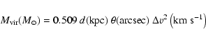
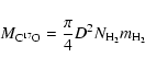
![\begin{displaymath}%
FWZI_{\rm Gauss}=\frac{FWHM}{\sqrt{\rm ln2}}\sqrt{{\rm ln}\left[\frac{T_{\rm max}}{3\sigma}\right]}\cdot
\end{displaymath}](/articles/aa/full/2005/12/aa1810/img114.gif)