A&A 432, 501-513 (2005)
DOI: 10.1051/0004-6361:20041355
Influence of magnification threshold on pixel lensing optical
depth, event rate and time scale distributions towards M 31
F. De Paolis 1 -
G. Ingrosso1 -
A. A. Nucita1 -
A. F. Zakharov2,3
1 - Dipartimento di Fisica, Università di Lecce and INFN, Sezione di
Lecce, CP 193, 73100 Lecce, Italy
2 -
Institute of Theoretical and Experimental Physics,
25, B. Cheremushkinskaya St., Moscow 117259, Russia
3 -
Astro Space
Centre of Lebedev Physics Institute, Moscow
Received 26 May 2004 / Accepted 2 November 2004
Abstract
Pixel lensing is the gravitational microlensing of light
from unresolved stars contributing to the luminosity flux
collected by a single pixel. A star must be sufficiently
magnified, that is, the lens impact parameter must be less than a
threshold value  if the excess photon flux in a pixel is to
be detected over the background. Assuming the parameters of the
Isaac Newton Telescope and typical observing conditions, we
present maps in the sky plane towards M 31 of threshold impact
parameter, optical depth, event number and event time scale,
analyzing in particular how these quantities depend on
in
pixel lensing searches. We use an analytical approach consisting
of averaging on
and the star column density the optical
depth, microlensing rate and event duration time scale. An overall
decrease in the expected optical depth and event number with
respect to the classical microlensing results is found,
particularly towards the high luminosity M 31 inner regions. As
expected, pixel lensing events towards the inner region of M 31 are
mostly due to self-lensing, while in the outer region dark events
dominate even for a 20% MACHO halo fraction. We also find a
far-disk/near-disk asymmetry in the expected event number, smaller
than that found by Kerins (2004). Both for self and dark lensing
events, the pixel lensing time scale we obtain is
if the excess photon flux in a pixel is to
be detected over the background. Assuming the parameters of the
Isaac Newton Telescope and typical observing conditions, we
present maps in the sky plane towards M 31 of threshold impact
parameter, optical depth, event number and event time scale,
analyzing in particular how these quantities depend on
in
pixel lensing searches. We use an analytical approach consisting
of averaging on
and the star column density the optical
depth, microlensing rate and event duration time scale. An overall
decrease in the expected optical depth and event number with
respect to the classical microlensing results is found,
particularly towards the high luminosity M 31 inner regions. As
expected, pixel lensing events towards the inner region of M 31 are
mostly due to self-lensing, while in the outer region dark events
dominate even for a 20% MACHO halo fraction. We also find a
far-disk/near-disk asymmetry in the expected event number, smaller
than that found by Kerins (2004). Both for self and dark lensing
events, the pixel lensing time scale we obtain is  1-7 days,
dark events lasting roughly twice as long as self-lensing
events. The shortest events are found to occur towards the M 31
South Semisphere. We also note that the pixel lensing results
depend on
1-7 days,
dark events lasting roughly twice as long as self-lensing
events. The shortest events are found to occur towards the M 31
South Semisphere. We also note that the pixel lensing results
depend on
 and
and
 values and ultimately on the observing conditions and telescope
capabilities.
values and ultimately on the observing conditions and telescope
capabilities.
Key words: gravitational lensing - Galaxy: halo - cosmology: dark matter -
galaxies: individual: M 31 - methods: observational
Pixel lensing surveys towards M 31 (Baillon et al. 1993; Crotts 1992) can
give valuable information to probe the nature of MACHOs (Massive
Astrophysical Compact Halo Objects) discovered in microlensing
experiments towards the LMC and SMC (Large and Small Magellanic
Clouds) (Aubourg et al. 1993; Alcock et al. 1993) and also address the question
of the fraction of halo dark matter in the form of MACHOs in
spiral galaxies (Alcock et al. 2000).
This may be possible due to both the increase in the number of
expected events and because the M 31 disk is highly inclined with
respect to the line of sight and so microlensing by MACHOs
distributed in a roughly spherical M 31 halo give rise to an
unambiguous signature: an excess of events on the far side of the
M 31 disk relative to the near side (Crotts 1992).
Moreover, M 31 surveys probe the MACHO distribution in a different
direction to the LMC and SMC and observations are made from the
North Earth hemisphere, probing the entire halo extension.
Table 1:
Parameters for the four M 31 models considered by
Kerins (2004). Columns are the model name, the component name,
the mass of the component, its central density  and the
adopted cut-off radius R. Additional columns give, where
appropriate, the core radius a, the disk scale length h and
height H, the flattening parameter q and the B-band
mass-to-light ratio
and the
adopted cut-off radius R. Additional columns give, where
appropriate, the core radius a, the disk scale length h and
height H, the flattening parameter q and the B-band
mass-to-light ratio
 in solar units.
The Pixel lensing technique studies the gravitational microlensing
of unresolved stars (Ansari et al. 1997). In a dense field of stars,
many of them contribute to each pixel. However, if one unresolved
star is sufficiently magnified, the increase of the total flux
will be large enough to be detected. Therefore, instead of
monitoring individual stars as in classical microlensing, one
follows the luminosity intensity of each pixel in the image. When
a significative (above the background and the pixel noise) photon
number excess repeatedly occurs, it is attributed to an ongoing
microlensing event if the pixel luminosity curve follows (as a
function of time) a Paczynski like curve (Paczynski 1996).
Clearly, variable stars could mimic a microlensing curve. These
events can be recognized by performing observations in several
spectral bands and monitoring the signal from the same pixel for
several observing seasons to identify the source.
Two collaborations, MEGA (preceded by the VATT/Columbia survey)
and AGAPE have produced a number of microlensing event candidates,
which show a rise in pixel luminosity in M 31 (Calchi Novati et al. 2002; Ansari et al. 1999; Auriere et al. 2001; Crotts & Tomaney 1996).
More recently, based on observations with the Isaac Newton
Telescope on La Palma (Kerins et al. 2001), the MEGA (de Jong et al. 2004),
POINT-AGAPE (Calchi Novati et al. 2003; Uglesich et al. 2004; Paulin-Henriksson et al. 2003) and WeCAPP
(Riffeser et al. 2003) collaborations claimed to find evidence of
several microlensing events.
In particular, the MEGA Collaboration (de Jong et al. 2004) presented the
first 14 M 31 candidate microlensing events, 12 of which are new
and 2 that have been reported by the POINT-AGAPE Collaboration
(Paulin-Henriksson et al. 2003). The preliminary analysis of the spatial and
timescale distribution of the events supports their microlensing
nature. In particular the far-disk/near-disk asymmetry, although
not highly significant, is suggestive of the presence of an M 31
dark halo.
The POINT-AGAPE Collaboration found in total a subset of four
short timescale, high signal-to-noise ratio microlensing
candidates, one of which is almost certainly due to a stellar lens
in the bulge of M 31 and the other three candidates can be
explained either by stars in M 31 and M 32, or by MACHOs.
In pixel lensing surveys, although all stars contributing to the same pixel
are candidates for a microlensing event, only the brightest stars
(usually blue and red giants) will be magnified enough to be
detectable above background fluctuations (unless for very high amplification
of main sequence stars, which are very unlikely events).
First evaluations have shown that the pixel lensing technique
towards M 31 may give rise to a significant number of events due to
the large number of stars contributing to the same pixel
(Han & Gould 1996; Gould 1994; Baillon et al. 1993; Jetzer 1994; Colley 1995).
Although these analytic estimates may be very rough, they provide
useful qualitative insights. To have reliable estimates in true
observational conditions one should use Monte-Carlo simulations
(Kerins et al. 2001; Ansari et al. 1997). In this way, given the capabilities of
the telescope and CCD camera used, the observing campaign and
weather conditions, one can estimate the event detection
efficiency as a function of event duration and maximum
amplification.
This study will be done in a forthcoming paper (De Paolis et al. 2004)
with the aim of investigating the lens nature (i.e. the population
to which the lens belongs) for the events discovered by MEGA
(de Jong et al. 2004) and POINT-AGAPE (Paulin-Henriksson et al. 2003).
In this paper, instead of using Monte-Carlo simulations, we
estimate the relevant pixel lensing quantities by analyzing the
effect of the presence of a magnification threshold (or,
equivalently, of a threshold impact parameter )
in pixel
lensing searches towards M 31. We use an analytic procedure
consisting of averaging the classical optical depth, microlensing
rate and event duration time scale on ,
which depends on the
magnitude of the source being magnified.
The paper is organized as follows. In Sect. 2 we briefly discuss
the source - bulge and disk stars in M 31 - and lens - stars in M 31
and in the Milky Way (MW) disk, MACHOs in M 31 and MW halos -
models we use. In Sect. 3 we discuss the pixel lensing
technique. In Sects. 4 and 5 we present maps of optical depth,
event rate and typical event time duration, addressing the
modification with respect to classical microlensing values, due to
the influence of the threshold magnification in pixel lensing
searches. Finally in Sect. 6 we present some conclusions.
The M 31 disk, bulge and halo mass distributions are described
adopting the parameters of the Reference model in Kerins (2004),
which provides remarkably good fits to the M 31 surface brightness
and rotation curve profiles.
This model, by using an average set of parameter values less
extreme with respect to the massive halo, massive bulge and
massive disk models in Table 1, can be considered a
more likely candidate model for the mass distributions in the M 31
galaxy.
Accordingly,
the mass density of the M 31 disk stars is described by
a sech-squared profile
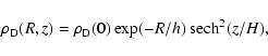 |
(1) |
where R is the distance on the M 31 disk plane,
 kpc and
 kpc are, respectively, the scale height and
scale lengths of the disk and
kpc are, respectively, the scale height and
scale lengths of the disk and
 kpc-3 is the central mass density. The disk is
truncated at
kpc-3 is the central mass density. The disk is
truncated at
 kpc so that the total mass is
 .
.
As usual, the M 31 disk is assumed to be inclined at the angle
 and the azimuthal angle relative to the near minor
axis
and the azimuthal angle relative to the near minor
axis
 .
.
The M 31 bulge is parameterized by a flattened power law of the
form
![\begin{displaymath}\rho_{\rm B}(R,z) = \rho_{\rm B}(0) \left[ 1+ \left( \frac {R}{a}\right)^2 +q^{-2}
\left( \frac {z}{a}\right)^2\right]^{-s/2},
\end{displaymath}](/articles/aa/full/2005/11/aa1355/img42.gif) |
(2) |
where the coordinates
x and y span the M 31 disk plane (z is perpendicular to it),
 kpc-3,
 is the ratio of the minor to major axes,
 kpc and
 (Reitzel et al. 1998).
The bulge is truncated at 40 kpc and its total mass
is
(Reitzel et al. 1998).
The bulge is truncated at 40 kpc and its total mass
is
 .
.
The dark matter in the M 31 halo is assumed to follow an isothermal
profile
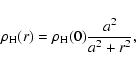 |
(3) |
with core radius
 kpc, and central dark matter density
 kpc-3, so that
the total rotational velocity in the M 31 halo is
kpc-3, so that
the total rotational velocity in the M 31 halo is
 km s-1. The M 31 halo is truncated at
 kpc
and the total dark mass within this distance is
kpc
and the total dark mass within this distance is
 .
.
As usual, the mass density profile for a MW disk is described with
a double exponential profile
 |
(4) |
with the Earth's position from the Galactic center at
 kpc, scale height
kpc, scale length
kpc, scale height
kpc, scale length
 kpc and local mass density
 kpc-3.
The MW bulge![[*]](/icons/foot_motif.gif) is described by the triaxial
bulge model with mass density profile (Dwek et al. 1995)
is described by the triaxial
bulge model with mass density profile (Dwek et al. 1995)
 |
(5) |
where
s4 = [(x/a)2+(y/b)2]2+(z/c)4, the bulge mass is
 and the scale lengths are
 kpc,
kpc,
 kpc and
 kpc.
Here, the coordinates x and y span the Galactic disk plane,
whereas z is perpendicular to it.
kpc.
Here, the coordinates x and y span the Galactic disk plane,
whereas z is perpendicular to it.
The dark halo in our Galaxy is also assumed to follow an
isothermal profile
with core radius
 kpc and local dark matter density
 kpc-3.
The corresponding total asymptotic rotational velocity
is
kpc-3.
The corresponding total asymptotic rotational velocity
is
 km s-1. The MW halo is truncated
at
kpc and the dark mass within this distance is
km s-1. The MW halo is truncated
at
kpc and the dark mass within this distance is
 .
.
For both M 31 and MW halos, the fraction of dark matter
in form of MACHOs is assumed to be
 (Alcock et al. 2000).
Moreover, as usual, we assume the random velocities of stars and
MACHOs to follow Maxwellian distributions with one-dimensional
velocity dispersion
 km s-1 and 30,
156 km s-1 for the M 31 disk, bulge, halo and MW disk and
halo, respectively (see also Kerins et al. 2001; An et al. 2004). In addition an
M 31 bulge rotational velocity of 30 km s-1 is assumed.
km s-1 and 30,
156 km s-1 for the M 31 disk, bulge, halo and MW disk and
halo, respectively (see also Kerins et al. 2001; An et al. 2004). In addition an
M 31 bulge rotational velocity of 30 km s-1 is assumed.
The main difference between gravitational microlensing and pixel
lensing observations relies in the fact that in pixel lensing a
large number of stars contribute to the same pixel and therefore
only bright and sufficiently magnified sources can be identified
as microlensing events. In pixel lensing analysis one usually
defines a minimum amplification that depends on the baseline
photon counts (Ansari et al. 1997)
 |
(6) |
which is the sum of the M 31 surface brightness and sky contribution.
The excess photon counts per pixel due to an ongoing microlensing event is
![\begin{displaymath}\Delta N_{\rm pix} = N_{\rm bl} [A_{\rm pix}-1] = f_{\rm see} N_{\rm s} [A(t)-1],
\end{displaymath}](/articles/aa/full/2005/11/aa1355/img70.gif) |
(7) |
where  and
and
 are the source and baseline photon
counts in the absence of lensing, A(t) is the source
magnification factor due to lensing and
are the source and baseline photon
counts in the absence of lensing, A(t) is the source
magnification factor due to lensing and
 is the
fraction of the seeing disk contained in a pixel.
is the
fraction of the seeing disk contained in a pixel.
As usual, the amplification factor is given by (see, e.g.,
Griest 1991, and references therein)
 |
(8) |
where
 |
(9) |
is the impact distance in units of the Einstein radius
![\begin{displaymath}R_{\rm E}=[(4Gm_{\rm l}/c^2) ~ D_{\rm l} (D_{\rm s}-D_{\rm l})/D_{\rm s}]^{1/2},
\end{displaymath}](/articles/aa/full/2005/11/aa1355/img75.gif) |
(10) |
and u0 is the impact parameter in units of  .
Moreover,
.
Moreover,
 is the Einstein time, t0 the time of
maximum magnification,
is the Einstein time, t0 the time of
maximum magnification,  and
and  are the source and lens
distances from the observer and
are the source and lens
distances from the observer and  is the lens transverse
velocity with respect to the line of sight.
is the lens transverse
velocity with respect to the line of sight.
The number of photons in a pixel is given by
 |
(11) |
and a pixel lensing event will be detectable if the excess pixel
photon counts
 are greater than the pixel
noise
are greater than the pixel
noise
 |
(12) |
 being the minimum noise level determined by the pixel
flux stability and
being the minimum noise level determined by the pixel
flux stability and
 the statistical photon
fluctuation.
the statistical photon
fluctuation.
By regarding a signal as being statistically significant
if it occurs at a level  above the baseline counts
,
one obtains
above the baseline counts
,
one obtains
 .
If
.
If  is taken equal to the minimum noise
level
,
the obtained threshold magnification
is taken equal to the minimum noise
level
,
the obtained threshold magnification  is (Kerins et al. 2001)
 |
(13) |
which corresponds to a threshold value
for the impact
distance via the relation in Eq. (8).
As one can see,
depends on the source magnitude M,
the line of sight to M 31 and the observing conditions.
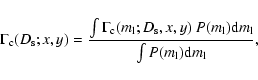
In pixel lensing analysis, the effect of the existence of
the threshold magnification (or, equivalently, of a threshold value
of the impact parameter) is usually taken
into account in estimating the pixel lensing rate (Kerins et al. 2001,2003)
 |
(14) |
where x and y are coordinates in the plane orthogonal to the
line of sight and
 is averaged
on the source magnitude M, namely
is averaged
on the source magnitude M, namely
 |
(15) |
M1-M2 (to be specified below) being the limiting values for
the source magnitude and
 the luminosity function,
i.e. the number density of sources in the absolute magnitude
interval
the luminosity function,
i.e. the number density of sources in the absolute magnitude
interval
 .
.
Pixel lensing event detection is usually performed in R or I bands
in order to minimize light absorption by the intervening dust
in M 31 and MW disks. Indeed, these bands offer the best compromise between
sampling and sky background, while other bands (B and V) are commonly used
to test achromaticity of the candidate events.
In the present analysis, as reference values, we adopt the
parameters of the Sloan-r filter on the Wide-Field Camera of the
Isaac Newton Telescope (Kerins et al. 2001). Therefore, since the red
giants are the most luminous stars in the red band,
we may safely assume that the overwhelming majority of the pixel
lensing event sources are red giants. Moreover, gives the lack of
precise information about the stellar luminosity function in the
M 31 galaxy, we assume that the same function  holds both
for the Galaxy and M 31 and does not depend on position.
holds both
for the Galaxy and M 31 and does not depend on position.
Accordingly, in the range of magnitude
 the
stellar luminosity function is proportional to the following
expression (Mamon & Soneira 1982)
the
stellar luminosity function is proportional to the following
expression (Mamon & Soneira 1982)
![\begin{displaymath}\phi(M) \propto
\frac{ 10^{\beta(M-M^*)} }
{ [ 1+10^{-(\alpha-\beta)\delta(M-M^*)}]^{1/\delta} },
\end{displaymath}](/articles/aa/full/2005/11/aa1355/img97.gif) |
(16) |
where, in the red band,
M*= 1.4,
 ,
,
 and
and
 .
.
On the other hand, the fraction of red giants (over the total star number)
as a function of Mcan be approximated as (Mamon & Soneira 1982)
where, in the red band,
 ,
,
 ,
,
 and
and
 .
Therefore, the fraction of red giants
averaged over the magnitude is given by
.
Therefore, the fraction of red giants
averaged over the magnitude is given by
 |
(18) |
from which we obtain
 .
.
Averaging the pixel lensing rate in Eq. (14)
on the source density we obtain
 |
(19) |
where the mean classical rate
 is
is
 |
(20) |
In turn, for a fixed source distance,
 is
obtained by the classical microlensing rate for
a lens of mass
is
obtained by the classical microlensing rate for
a lens of mass  (Griest 1991),
by averaging on the lens mass, namely
(Griest 1991),
by averaging on the lens mass, namely
 |
(21) |
where
 is the lens mass distribution function.
For lenses belonging to the bulge and disk star populations,
lenses are assumed to follow a broken power law
(see e.g. An et al. 2004, and references therein)
where the upper limit
 is
is
 for M 31 bulge stars and
 for M 31 and MW disk stars.
The resulting mean mass for lenses in the bulges and disks are
for M 31 and MW disk stars.
The resulting mean mass for lenses in the bulges and disks are
 and
and
 ,
respectively.
,
respectively.
For the lens mass in the M 31 and MW halos we
assume the  -function approximation and we take
a MACHO mass
-function approximation and we take
a MACHO mass
 ,
according to the mean value
in the analysis of
microlensing data
towards LMC (Alcock et al. 2000).
,
according to the mean value
in the analysis of
microlensing data
towards LMC (Alcock et al. 2000).
As usual, the mean number of expected events in classical microlensing
 and pixel lensing
 ,
respectively,
are related to the observation time
,
respectively,
are related to the observation time
 ,
source column density
and mean fraction of red giants
,
source column density
and mean fraction of red giants
 by
by
 |
(23) |
 |
(24) |
where the source column density is
 |
(25) |
However, the classical microlensing rate depends on several source
and lens parameters, in particular on the lens mass and transverse
velocity of the source and lens. Therefore, due to the parameter
degeneracy, it does not give precise information on the lens
population, at least in the M 31 regions where microlensing by
stars in M 31 itself (self-lensing) and by MACHOs in M 31 and MW
halos (dark lensing) occur with comparable probability. Indeed, as
usual, the probability for a given lens population is
 |
(26) |
On the other hand, the classical microlensing optical depth
 |
(27) |
is a geometrical quantity and depends on a small number of
parameters and can be used as in Eq. (26) to determine the
lens nature.
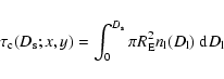
Physically the optical depth is the number of ongoing microlensing
events per source star at any instant in time. So, one can also
compute the instantaneous event number density, as a function of
position, by multiplying the optical depth by the number density
of sources
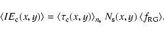 |
(28) |
However, Eq. (27) is the usual definition for the optical
depth in classical gravitational microlensing, while in the case
of pixel lensing it is necessary to take into account the effect
of
 .
.
In order to generalize the  definition to the pixel lensing
case, a new definition (which joins the advantage of using a
geometrical quantity with the main characteristic of the pixel
lensing technique, i.e. the effect of the baseline) is introduced
(see also Kerins 2004)
definition to the pixel lensing
case, a new definition (which joins the advantage of using a
geometrical quantity with the main characteristic of the pixel
lensing technique, i.e. the effect of the baseline) is introduced
(see also Kerins 2004)
 |
(29) |
where
 is
is
 |
(30) |
The factor
 in Eq. (29) comes from the consideration that the Einstein radius
,
which enters quadratically in
in Eq. (29) comes from the consideration that the Einstein radius
,
which enters quadratically in
 ,
has to be
multiplied by
(always less than unity for pixel lensing).
,
has to be
multiplied by
(always less than unity for pixel lensing).
Accordingly, the instantaneous event number density in pixel lensing is
given by
 |
(31) |
Here we note that in evaluating
for
each model considered in Table 1, we have to take into
account that the number of detectable pixel lensing events does
not depends on the typical source luminosity  to first
order (Kerins 2004). Indeed, although for a fixed source
luminosity
the number of sources
to first
order (Kerins 2004). Indeed, although for a fixed source
luminosity
the number of sources
 ,
the
pixel lensing rate per source
,
the
pixel lensing rate per source
 , so that the event
number does not depend on .
The same also holds for the
instantaneous event number density
, so that the event
number does not depend on .
The same also holds for the
instantaneous event number density
 .
.
In pixel microlensing, due to the large number of stars
simultaneously contributing to the same pixel, the flux from a
single star in the absence of lensing is generally not observable.
Thus, the Einstein time  cannot be determined reliably by
fitting the observed light curve.
cannot be determined reliably by
fitting the observed light curve.
Indeed, another estimator of the event time duration has been
proposed, namely the full-width half-maximum event duration
tFWHM, which depends on
and u0 (Gondolo 1999)
 |
(32) |
where w(u0) is given by
![\begin{displaymath}w(u_0) = 2 \sqrt{2 f [f(u_0^2)]-u_0^2}
\end{displaymath}](/articles/aa/full/2005/11/aa1355/img155.gif) |
(33) |
and
f(x) = A(x) - 1,
where A(x) is the amplification factor in Eq. (8).
This quantity can be put in a different form (Kerins et al. 2001)
 |
(34) |
where
 .
.
In the limit of large amplification
 (or, equivalently,
 )
one obtains
)
one obtains
 |
(35) |
Using Eqs. (35) in (34),
the full-width half-maximum event duration can be
approximated by
 |
(36) |
Clearly, while in classical microlensing u0 may be determined,
in pixel microlensing the background overcomes the source baseline
making u0 unknown, implying that an average procedure on u0is needed to estimate the mean event duration. Since the impact
parameter u0 varies in the range
 and the probability
of u0 being in the range u0 -
and the probability
of u0 being in the range u0 -
 is
is
 (the area of the circular ring of radius
u0 and thickness
(the area of the circular ring of radius
u0 and thickness
 ), by averaging tFWHM on the impact
parameter, in the limit of large amplification, one gets
), by averaging tFWHM on the impact
parameter, in the limit of large amplification, one gets
 |
(37) |
where
 |
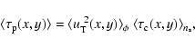
(38) |
Inspection of the relation in Eq. (37) and
of Eqs. (14), (19)
and (29),
lead us to introduce for pixel lensing a new event time scale estimator
 defined as
 |
(39) |
where
 |
(40) |
and
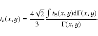 |
(41) |
Clearly, the pixel lensing time scale
turns out to be the full-width half-maximum event duration
averaged over the impact parameter.
Before discussing the results obtained, we summarize some
assumptions used in the present analysis. First, we assume perfect
sensitivity to pixel lensing event detection in M 31 pixel lensing
searches. Moreover, as reference values, we use the parameters for
the Isaac Newton Telescope and WFC (Wide-Field Camera) adopted by
the POINT-AGAPE collaboration (Kerins et al. 2001,2003).
The Telescope diameter, the pixel field of view and the image
exposition time are 2.5 m, 0.33 arcsec and
 s,
respectively. We also assume a gain or conversion factor of 2.8 e-/ADU, and a loss factor 3, both for atmospheric
and instrumental effects. The zero-point with the Sloan-r WFC is
s,
respectively. We also assume a gain or conversion factor of 2.8 e-/ADU, and a loss factor 3, both for atmospheric
and instrumental effects. The zero-point with the Sloan-r WFC is
 24.3 mag arcsec-2.
To take into account the effect of seeing, we employ an analysis
based on superpixel photometry. Adopting a value of 2.4 arcsec for
the worst seeing value, we take a superpixel dimension of  pixel
and adopt a minimum noise level of
pixel
and adopt a minimum noise level of
 .
We also assume that typically 87 per cent of
a point spread function (PSF) positioned at the center of a
superpixel is contained within the superpixel itself.
.
We also assume that typically 87 per cent of
a point spread function (PSF) positioned at the center of a
superpixel is contained within the superpixel itself.
The considered sky background is
 mag arcsec-2
(corresponding to a Moon eclipse), so that the
typical sky luminosity is
mag arcsec-2
(corresponding to a Moon eclipse), so that the
typical sky luminosity is
 counts/pixel,
which enters in the baseline count estimates. However, for
comparison purposes with Kerins (2004), some results in Tables 3-5
are also given for a
sky background
counts/pixel,
which enters in the baseline count estimates. However, for
comparison purposes with Kerins (2004), some results in Tables 3-5
are also given for a
sky background
 mag arcsec-2 and
 (corresponding to a randomly positioned PSF
within the superpixel).
(corresponding to a randomly positioned PSF
within the superpixel).
Moreover, all the figures presented in Sect. 6 are given
for the Reference model (see Table 1).
The effect of varying the model parameters
for the M 31 bulge, disk and halo is also shown in Tables 3-5.
Finally, we recall that
 is obtained from Eq. (6) where
 follows from the M 31
photometry given by Kent (1989).
follows from the M 31
photometry given by Kent (1989).
In Fig. 1 maps of the mean threshold impact parameter
and
towards M 31 are shown.
![\begin{figure}
\par\includegraphics[width=7.5cm,clip]{1355fig1.eps}\end{figure}](/articles/aa/full/2005/11/aa1355/Timg181.gif) |
Figure 1:
The mean impact parameter maps
and
towards M 31 are given, for selected
directions towards M 31 corresponding to different (x,y)coordinates (in units of arcmin) centered on M 31 and aligned along
the major and minor axes of the projected light profile. |
| Open with DEXTER |
In this and following figures we use Cartesian coordinates x and
y centered on M 31 and aligned along the major and minor axes of
the projected light profile, respectively.
As one can see in Fig. 1, the effect of the higher
luminosity of the inner region of M 31 with respect to the outer
part of the galaxy is to reduce the obtained
values by about an order of magnitude.
![\begin{figure}
\par\includegraphics[width=8cm,clip]{1355fig2.eps}\end{figure}](/articles/aa/full/2005/11/aa1355/Timg182.gif) |
Figure 2:
The mean impact parameter
is given as a function of the
background photon counts
 in a pixel, for selected
directions towards M 31 corresponding to different (x,y)coordinates (in units of arcmin) in the sky plane. Thin lines, from
the bottom to the upper part of the figure, refer to (8,0),
(16,0) and (32,0); thick lines are for (0,-2), (0,-4) and
(0,-8) coordinates, respectively.
in a pixel, for selected
directions towards M 31 corresponding to different (x,y)coordinates (in units of arcmin) in the sky plane. Thin lines, from
the bottom to the upper part of the figure, refer to (8,0),
(16,0) and (32,0); thick lines are for (0,-2), (0,-4) and
(0,-8) coordinates, respectively. |
| Open with DEXTER |
Table 2:
The threshold impact parameters
 and
and
 averaged over the
whole M 31 galaxy are given for different values of the superpixel
dimension
averaged over the
whole M 31 galaxy are given for different values of the superpixel
dimension
 ,
sky background
,
sky background
 ,
fraction
of the superpixel covered by the PSF and superpixel
flux stability
.
,
fraction
of the superpixel covered by the PSF and superpixel
flux stability
.
Table 3:
The expected number of events
 per
year in pixel lensing observations towards the M 31 galaxy for
different locations of sources and lenses is shown. We consider
the
per
year in pixel lensing observations towards the M 31 galaxy for
different locations of sources and lenses is shown. We consider
the
 arcmin2 region oriented along the major axis of M 31.
and exclude events occurring within a radius of 8 arcmin of the
M 31 center. Sources and lenses in the M 31 bulge and disk are
indicated by indices 1 and 2, while lenses in the M 31 halo and MW
disk and halo by indices 3, 5 and 6. The first and second indices
refer to source and lens, respectively. The mean mass of bulge and
disk stars is
arcmin2 region oriented along the major axis of M 31.
and exclude events occurring within a radius of 8 arcmin of the
M 31 center. Sources and lenses in the M 31 bulge and disk are
indicated by indices 1 and 2, while lenses in the M 31 halo and MW
disk and halo by indices 3, 5 and 6. The first and second indices
refer to source and lens, respectively. The mean mass of bulge and
disk stars is
 and
and
 ,
respectively. For the lenses in the M 31 and MW halos we take a
mass of
,
respectively. For the lenses in the M 31 and MW halos we take a
mass of
 and a MACHO fraction
 .
.
Table 4:
The same as in Table 3 for lenses located
in the M 31 galaxy. In the last three columns we give the
calculated pixel event number for the South/North Semisphere and
in brackets their ratio.
Table 5:
The instantaneous number of events in pixel lensing
observations towards the M 31 galaxy for different locations of
sources and lenses is shown (for details see text). Numbers in
brackets refer to the South Semisphere of M 31. For the MW disk and
halo, lenses in the South Semisphere of the MW contribute to
roughly one half of the total and so the corresponding event
numbers are not given.
In Fig. 2, for selected lines of sight to M 31, we show
how
depends on the photon
counts
from the background, which is approximated as
a diffuse source of magnitude
in the range
20.9-18.9 mag arcsec-2. In Fig. 2 we consider several
lines of sight to M 31 with different (x,y) coordinates (in units
of arcmin) in the orthogonal plane. Thin lines, from the bottom to
the top, refer to (0,-0.2), (4,-0.2) and (8,-0.2), thick
lines are for (0,-2), (4,-2) and (8,-2) coordinates. It is
evident that
weakly depends on
in the inner M 31 regions, where
is
dominated by the counts
 from the M 31 surface
brightness. Moreover, for a fixed number of counts
from the sky,
decreases with
increasing
.
from the M 31 surface
brightness. Moreover, for a fixed number of counts
from the sky,
decreases with
increasing
.
We note that by averaging
and
(weighting with the star
number density) on the whole field of view towards the M 31 galaxy,
we obtain
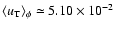 and
and
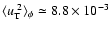 .
.
In Table 2 the effect on
and
of changing
the parameter values for the superpixel dimension
,
,
and
is shown. This is
relevant since, referring to the subsequent Tables 3-5, one can verify that the results for the
Reference model (in the last two rows) scale with
(in Tables 3 and 4) and
(last four rows in Table 5). Therefore, since
and
strongly depend on the
above mentioned parameters, we expect that all pixel lensing
estimated quantities heavily depend on the observing conditions
and telescope capabilities.
![\begin{figure}
\par$\begin{array}{c@{\hspace{0.4in}}c} \epsfxsize=3.25in
\epsfys...
...3b.eps}\\ [0.cm]
\mbox{\bf a)} & \mbox{\bf b)}
\end{array}$\par
\par\end{figure}](/articles/aa/full/2005/11/aa1355/Timg211.gif) |
Figure 3:
Mean optical depth
 maps (in
units of 10-6) towards M 31 are given for selected source and
lens populations. The first index refers to the source stars (1
for M 31 bulge, 2 for M 31 disk) while the second one refers to the
lens populations (1 and 2 as above, 3 for MACHOs in the M 31 halo).
Optical depth maps for lenses belonging to the MW disk and halo
populations are not given since the obtained results are almost
constant in any direction.
maps (in
units of 10-6) towards M 31 are given for selected source and
lens populations. The first index refers to the source stars (1
for M 31 bulge, 2 for M 31 disk) while the second one refers to the
lens populations (1 and 2 as above, 3 for MACHOs in the M 31 halo).
Optical depth maps for lenses belonging to the MW disk and halo
populations are not given since the obtained results are almost
constant in any direction. |
| Open with DEXTER |
![\begin{figure}
\par$\begin{array}{c@{\hspace{0.4in}}c} \epsfxsize=3.25in
\epsfys...
...55fig4b.eps}\\ [0.cm]
\mbox{\bf a)} & \mbox{\bf b)}
\end{array}$\par\end{figure}](/articles/aa/full/2005/11/aa1355/Timg213.gif) |
Figure 4:
In panel a), the mean classical optical depth
maps
(in units of 10-6) towards M 31 are given for self, dark and total
lensing. In panel b), the mean pixel lensing optical depth
 maps
are given, in the same cases.
maps
are given, in the same cases.
|
| Open with DEXTER |
Classical microlensing optical depth maps for selected M 31 source and lens
populations are shown in Fig. 3 for the Reference model.
Here and below, sources and lenses in the M 31 bulge and disk are
indicated by indices 1 and 2, while lenses in the M 31 halo and MW
disk and halo by indices 3, 5 and 6. The first and second indices
refer to source and lens, respectively.
As one can see,
always increases
towards the M 31 center. The well-known far-to-near side asymmetry
of the M 31 disk is clearly demonstrated in
 ,
where the lenses are in the M 31 halo.
Moreover, a strong asymmetry in the opposite direction in the
bulge-disk (12) and disk-bulge (21) events (due to the relative
source-lens location) is also evident.
,
where the lenses are in the M 31 halo.
Moreover, a strong asymmetry in the opposite direction in the
bulge-disk (12) and disk-bulge (21) events (due to the relative
source-lens location) is also evident.
We have also found that the classical mean optical depth
for lenses in our Galaxy (
 ,
,
 ,
,
 and
and
 )
is almost constant in any direction and therefore we do not show
the corresponding maps. For reference, the obtained values are
)
is almost constant in any direction and therefore we do not show
the corresponding maps. For reference, the obtained values are
 and
and
 .
.
In Fig. 4a classical optical depth maps towards M 31 are
given for self-lensing (
 )
and dark-lensing
(
)
and dark-lensing
(
 ). The
total contribution
). The
total contribution
 is given
at the bottom of the same figure.
is given
at the bottom of the same figure.
We notice that, in order to evaluate
 and
and
 ,
we sum optical depths obtained for different source
populations and therefore the averaging procedure
in Eq. (30) is done
by normalizing with the factor
,
we sum optical depths obtained for different source
populations and therefore the averaging procedure
in Eq. (30) is done
by normalizing with the factor
![$\int [n_1(D_{\rm s};x,y)+n_2(D_{\rm s};x,y)] {\rm d}D_{\rm s}$](/articles/aa/full/2005/11/aa1355/img226.gif) .
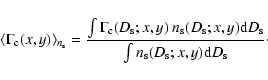
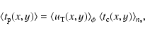
Mean pixel lensing optical depth
maps are shown in Fig. 4b.
.
Mean pixel lensing optical depth
maps are shown in Fig. 4b.
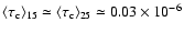
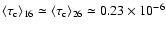
As we can see, the main effect of the threshold impact parameter
is to substantially decrease
(with
respect to
values) in particular
towards the central regions of M 31, as a consequence of the
increasing luminosity. Indeed, on average
 and
and
 (see the
third row in Table 2) for the parameter values used in
the figures.
(see the
third row in Table 2) for the parameter values used in
the figures.
![\begin{figure}
\par$\begin{array}{c@{\hspace{0.4in}}c} \epsfxsize=3.25in
\epsfys...
...55fig5b.eps}\\ [0.cm]
\mbox{\bf a)} & \mbox{\bf b)}
\end{array}$\par\end{figure}](/articles/aa/full/2005/11/aa1355/Timg229.gif) |
Figure 5:
In panel a), the instantaneous pixel lensing event number density
maps
(events per arcmin2) towards M 31 are given for self, dark and total
lensing.
In panel b) maps of pixel lensing event rate
(events per year and per arcmin2) are given,
in the same cases. |
| Open with DEXTER |
Maps of the expected number of events in pixel lensing surveys
towards M 31 are shown in Fig. 5 for the Reference model.
As for the optical depth, we give the number of events separately
for self-lensing, dark-lensing and also the total contribution.
In Figs. 5a and 5b we show, as a function of
position, maps of the instantaneous event number density
(events per arcmin2) and the event rate
(events per year and arcmin2).
or the optical depth, the effect of the threshold impact parameter
is to produce a decrease of the event number density towards the
M 31 center (for
 arcmin) and an overall reduction of
the event number density with respect to the expectations from
classical microlensing results. Moreover, in the figures it is
also evident that the inner region (within about 10 arcmin from
the M 31 center) is dominated by self-lensing events.
arcmin) and an overall reduction of
the event number density with respect to the expectations from
classical microlensing results. Moreover, in the figures it is
also evident that the inner region (within about 10 arcmin from
the M 31 center) is dominated by self-lensing events.
In Fig. 7 the projected (along the x axis) mean event
number density
 as a function of the
coordinate y is given. The dashed line refers to dark lensing
events by MACHOs in M 31 and MW halos while the solid line is for
self-lensing events by stars in M 31 bulge and disk. The
North/South asymmetry is evident for dark events that are
relatively more numerous in the South Semisphere, corresponding to
the far side of the M 31 disk.
as a function of the
coordinate y is given. The dashed line refers to dark lensing
events by MACHOs in M 31 and MW halos while the solid line is for
self-lensing events by stars in M 31 bulge and disk. The
North/South asymmetry is evident for dark events that are
relatively more numerous in the South Semisphere, corresponding to
the far side of the M 31 disk.
![\begin{figure}
\par$\begin{array}{c@{\hspace{0.4in}}c} \epsfxsize=3.25in
\epsfys...
...55fig6b.eps}\\ [0.cm]
\mbox{\bf a)} & \mbox{\bf b)}
\end{array}$\par\end{figure}](/articles/aa/full/2005/11/aa1355/Timg233.gif) |
Figure 6:
In panel a), mean classical event duration time
 (in days) maps towards M 31 are given for self,
dark and total lensing. In panel b) for pixel lensing, maps of
are given, in the same cases.
(in days) maps towards M 31 are given for self,
dark and total lensing. In panel b) for pixel lensing, maps of
are given, in the same cases. |
| Open with DEXTER |
In Table 3, for selected locations of sources
(stars in M 31 bulge and disk) and lenses
(stars in M 31 bulge and disk, stars in MW disk
and MACHOs in M 31 and MW halos)
we give the expected total number of events detectable
by monitoring for 1 year the
arcmin2 region oriented along the
major axis of M 31 (events within 8 arcmin from the center are excluded).
The first four lines refer to the models considered in Table 1
and to the parameters in the third row of Table 2.
As one can see, the obtained results for the Reference model
are intermediate with respect to those for the other more extreme models.
In the last row of Table 3, for the Reference model we
show how the expected event number changes considering a different
value of
 (see 5th row in Table 2). As expected, one
can verify that roughly the event number scales as
.
(see 5th row in Table 2). As expected, one
can verify that roughly the event number scales as
.
Similar results have been obtained in previous simulations (see,
e.g. Kerins 2004, and references therein). We also note that
our numerical results scale with the fraction of halo dark matter
in form of MACHOs and with the MACHO mass by a factor
 .
.
In Table 4 we give the total event number
for different lens populations (bulge, disk and halo)
located in M 31. As one can see, the ratio dark/total events
depends on the considered model, varying from 0.07 (for the
massive disk model) to 0.40 for the massive halo model.
To study the far-disk/near-disk asymmetry, in the last three
columns of Table 4 we give results for the South/North
M 31 Semispheres and in brackets their ratio. For the Reference
model, we find that self-lensing events are roughly symmetric (the
same is true for lenses located in the MW disk and halo, not given
in the table), while events due to lenses in M 31 halo are
asymmetrically distributed with a ratio of about 2. The asymmetry
is particularly evident (in the last column of the table) for
sources located in the disk.
In Table 5 the instantaneous total number of events
 within the considered M 31 region is given.
The first four rows refer to the parameter values
within the considered M 31 region is given.
The first four rows refer to the parameter values
 ,
,
 ,
,
 and
and
 (used throughout the
paper). For comparison with the results obtained by
Kerins (2004), in the last four rows of Table 5 we
present our results for
(used throughout the
paper). For comparison with the results obtained by
Kerins (2004), in the last four rows of Table 5 we
present our results for
 ,
,
 ,
,
 and
and
 .
The asymmetry ratio we obtain is always rather
smaller than that quoted by Kerins (2004).
.
The asymmetry ratio we obtain is always rather
smaller than that quoted by Kerins (2004).
As it has been mentioned by several authors, in order to
discriminate between self and dark lensing events, it is important
to analyze the event duration. Indeed self-lensing events are
expected to have, on average, shorter duration with respect to
events due to halo MACHOs.
![\begin{figure}
\par\includegraphics[width=8cm,clip]{1355fig7.eps}\end{figure}](/articles/aa/full/2005/11/aa1355/Timg246.gif) |
Figure 7:
The projected (along the xaxis) mean event number
 is given as a
function of the coordinate y for the Reference model. The dashed
line refers to dark lensing events by MACHOs in M 31 and MW halos
while the solid line is for self-lensing events by stars in M 31
bulge and disk.
is given as a
function of the coordinate y for the Reference model. The dashed
line refers to dark lensing events by MACHOs in M 31 and MW halos
while the solid line is for self-lensing events by stars in M 31
bulge and disk. |
| Open with DEXTER |
Maps of mean event duration time scale in classical and pixel lensing are
shown in Figs. 6a and 6b.
Here we use the probability, for each location of sources and
lenses given in Eq. (26), of obtaining event duration maps
for self and dark microlensing events.
As expected, short duration events are mainly distributed towards
the inner regions of the galaxy and this occurs for both
and
.
The main effect
of
is to decrease the event time
scale, in particular towards the inner regions of M 31, giving a
larger number of short duration events with respect to
expectations based on
calculations.
Both for self and dark events the pixel lensing time scale we
obtain is 1- 7 days, in agreement with results in
Kerins (2004), but much shorter with respect to the duration of
the events observed by the MEGA Collaboration (de Jong et al. 2004). This
is most likely due to the fact that current experiments may not
detect events shorter than a few days.
However, the pixel lensing time scale values depend on
and ultimately on the observational
conditions and the adopted analysis procedure. Indeed from Table 2 one can see that the
value may be easily doubled, changing the adopted
parameters and therefore giving longer events.
In Fig. 8 the pixel lensing event duration
 averaged along the x direction
is given as a function of the y coordinate.
The dashed line refers to dark lensing events by MACHOs in M 31 and MW halos
while the solid line is for self-lensing events by stars in M 31 bulge and disk.
averaged along the x direction
is given as a function of the y coordinate.
The dashed line refers to dark lensing events by MACHOs in M 31 and MW halos
while the solid line is for self-lensing events by stars in M 31 bulge and disk.
![\begin{figure}
\par\includegraphics[width=8cm,clip]{1355fig8.eps}\end{figure}](/articles/aa/full/2005/11/aa1355/Timg249.gif) |
Figure 8:
The pixel lensing event
duration
 averaged along the xdirection is given as a function of the y coordinate. The dashed
line refers to dark lensing events by MACHOs in M 31 and MW halos
while the solid line is for self-lensing events by stars in M 31
bulge and disk.
averaged along the xdirection is given as a function of the y coordinate. The dashed
line refers to dark lensing events by MACHOs in M 31 and MW halos
while the solid line is for self-lensing events by stars in M 31
bulge and disk. |
| Open with DEXTER |
It is clearly evident that dark events last roughly twice as long
as self-lensing events and that the shortest events are expected
to occur towards the M 31 South Semisphere.
The presence of a large number of short duration events in pixel
lensing experiments towards M 31 has been reported by several
authors (Paulin-Henriksson et al. 2003; Paulin-Henriksson 2004).
We have studied the optical depth, event number and time scale
distributions in pixel lensing surveys towards M 31 by addressing,
in particular, the changes with respect to expectations from
classical microlensing (in which the sources are resolved).
Assuming, as reference values, the capabilities of the Isaac
Newton Telescope in La Palma and typical CCD camera parameters,
exposure time and background photon counts, we perform an analysis
consisting of averaging all relevant microlensing quantities over
the threshold value
 of the impact parameter. Clearly,
as in classical microlensing estimates, an average procedure is
also done with respect to all the other parameters entering in
microlensing observables: source and lens position, lens mass and
source and lens transverse velocities.
of the impact parameter. Clearly,
as in classical microlensing estimates, an average procedure is
also done with respect to all the other parameters entering in
microlensing observables: source and lens position, lens mass and
source and lens transverse velocities.
The M 31 bulge, disk and halo mass distributions are described
following the Reference model in Kerins (2004), which provides
remarkably good fits to the M 31 surface brightness and rotation
curve profiles. We also take a standard mass distribution model
for the MW galaxy, as described in Sect. 2, and assume that M 31
and MW halos contain 20% 0.5  MACHOs.
We consider red giants as the sources that most likely may be
magnified (and detected in the red band) in microlensing surveys.
Moreover, given the lack of precise information about the stellar
luminosity function in M 31, we assume that the same function holds
both for the Galaxy and M 31 and does not depend on the position.
Accordingly, the fraction of red giants (over the total star
number) is
 .
.
Our main results are maps in the sky plane towards M 31
of threshold impact parameter
,
optical depth
,
instantaneous event number density
(events per arcmin2 of ongoing microlensing events at any instant
in time)
and event number density
(events per yr and arcmin2 to be detected in M 31 surveys)
and time scale
.
These maps show an overall reduction of the corresponding classical
microlensing results and also a distortion of their shapes with respect
to other results in the literature.
Figures 3 and 4 show maps of the mean optical
depth (averaged over the source number density) for the different
source and lens locations.
In Fig. 5 we give the instantaneous pixel lensing
event number density and the event rate for self, dark and total
lensing. It clearly appears that the central region of M 31
is dominated by self-lensing events due to sources and lenses in M 31 itself,
while dark events are relatively more numerous in the outer region
(see also Fig. 7).
In Tables 3 and 4, for the M 31 mass distribution
models considered by Kerins (2004), we give the expected total
event number
to be detected by monitoring,
for 1 yr, the
arcmin2 region oriented along the major
axis of M 31 (the inner 8 arcmin region is excluded). We find that
the expected dark to total event number ratio is between 7% (for
the massive disk model) and 40% (for the massive halo model). The
tables also show the well-known far-disk/near-disk asymmetry due
to lenses in the M 31 halo. Self-lensing events, instead, are
distributed more symmetrically between the M 31 North and South
Semisphere. Similar conclusions are evident from Table 5, where we give the instantaneous number of events,
although the asymmetry ratio we obtain is always smaller than the
values quoted by Kerins (2004).
Figure 6 shows a decrease of the event time scale with
respect to classical microlensing, particularly towards the inner
regions of M 31, due to the high brightness of the galaxy. Both for
self and dark lensing events, the pixel lensing time scale we
obtain is 1-7 days, in agreement with results in the
literature. Note that the duration of the events observed by the
MEGA Collaboration (de Jong et al. 2004) is typically much longer than 7 days, due to the difficulty of detecting short events in current
experiments. It is also clear from Fig. 6 that dark
events last roughly twice as long as self-lensing events and that
the shortest events are expected to occur towards the M 31 South
Semisphere (see Fig. 8).
However, we emphasize that the pixel lensing results obtained
depend on
and
values, and ultimately on the
observing conditions and telescope capabilities. Indeed, from
Table 2, where the values of
and
averaged over the
whole M 31 galaxy are given, one can verify that pixel lensing
quantities scaling with
(
and
 )
may vary by more than one
order of magnitude while quantities scaling with
(
)
may vary by more than one
order of magnitude while quantities scaling with
(
 and
)
may change by two orders of magnitude.
and
)
may change by two orders of magnitude.
The present analysis can be used to test estimates and Monte-Carlo
simulations by other Collaborations and it has also been performed
in view of a planned survey towards M 31 by the SLOTT-AGAPE
Collaboration (Bozza et al. 2000).
Acknowledgements
We acknowledge S. Calchi Novati, Ph. Jetzer and F. Strafella
for useful discussions.
- Alcock, C.,
Akerloff, C. W., Allsman, R. A., et al. 1993,
Nature, 365, 621 [NASA ADS] [CrossRef]
- Alcock, C.,
Allsman, R. A., Alves, D. R., et al. 2000, ApJ, 542,
281 [NASA ADS] [CrossRef] (In the text)
- Ansari, R.,
Auriere, M., Baillon, P., et al. 1995, in Proc. of the XVII
Texas Symp., Annals of the N.Y. Academy of Sciences, ed. Bohringer
H., Morfill G. E., & Trumper J. E., 759, 608
- Ansari, R.,
Auriere, M., Baillon, P., et al. 1997, A&A, 324, 843 [NASA ADS] (In the text)
- Ansari, R.,
Auriere, M., Baillon, P., et al. 1999, A&A, 344, L49 [NASA ADS]
- An, J. H., Evans, N. W.,
Kerins, E., et al. 2004, ApJ, 601, 845 [NASA ADS] [CrossRef]
- Aubourg, E.,
Bareyre, P., Brehin, S., et al. 1993, Nature, 365, 623 [NASA ADS] [CrossRef]
- Auriere, M.,
Baillon, P., Bouquet, A., et al. 2001, ApJ, 553, L137 [NASA ADS] [CrossRef]
- Baillon, P.,
Bouquet, A., Giraud-Heraud, Y., & Kaplan, J. 1993, A&A,
277, 1 [NASA ADS]
- Baltz, E. A., Gyuk,
G., & Crotts, A. P. S. 2003, ApJ, 582, 30 [NASA ADS] [CrossRef]
- Bozza, V., Calchi
Novati, S., Capaccioli, M., et al. 2000, Mem.
Soc. Astron. It., 71, 1113 [NASA ADS] (In the text)
- Calchi Novati, S.,
Iovane, G., Marino, A., et al. 2002, A&A, 381, 845 [NASA ADS]
- Calchi Novati, S.,
Jetzer, Ph., Scarpetta, G., et al. 2003, A&A, 405,
851 [EDP Sciences] [NASA ADS] [CrossRef]
- Caon, N.,
Capaccioli, M., & D'Onofrio, M. 1993, MNRAS 265, 1013
- Colley, W. N. 1995,
AJ, 109, 440 [NASA ADS] [CrossRef]
- Crotts, A. P. S.
1992, ApJ, 399, L43 [NASA ADS] [CrossRef]
- Crotts, A. P. S.,
& Tomaney, A. B. 1996, ApJ, 473, L87 [NASA ADS] [CrossRef]
- de Jong, J. T. A.,
Kuijken, K., Crotts, A. P. S., et al. 2004, A&A, 417,
461 [EDP Sciences] [NASA ADS] [CrossRef] (In the text)
- De Paolis, F.,
Ingrosso, G., Nucita, A., et al. 2004, in preparation
(In the text)
- Dwek, E., Arendt, R.
G., Hauser, M. G., et al. 1995, ApJ, 445, 716 [NASA ADS] [CrossRef] (In the text)
- Giudice, G. F.,
Mollerach, S., & Roulet, E. 1994, Phys. Rev. D, 50, 4 [CrossRef]
- Gondolo, P. 1999,
ApJ, 510, L29 [NASA ADS] [CrossRef] (In the text)
- Gould, A. 1994, ApJ,
435, 573 [NASA ADS] [CrossRef]
- Griest, K. 1991, ApJ,
366, 412 [NASA ADS] [CrossRef] (In the text)
- Gyuk, G., & Crotts,
A. P. S. 2000, ApJ, 535, 621 [NASA ADS] [CrossRef]
- Han, C., & Gould, A.
1996, ApJ, 473, 230 [NASA ADS] [CrossRef]
- Jetzer, Ph. 1994,
A&A, 286, 426 [NASA ADS]
- Kent, S. M. 1989, AJ, 97,
1614 [NASA ADS] [CrossRef] (In the text)
- Kerins, E., Carr,
B., Ewans, N.W., et al. 2001, MNRAS, 323, 13 [NASA ADS] [CrossRef] (In the text)
- Kerins, E., An, J.,
Ewans, N. W., et al. 2003, ApJ, 598, 993 [NASA ADS] [CrossRef]
- Kerins, E. 2004,
MNRAS, 347, 1033 [NASA ADS] [CrossRef] (In the text)
- Mamon, G.
A., & Soneira, R. M. 1982, ApJ, 255, 181 [NASA ADS] [CrossRef] (In the text)
- Paczynski, B.
1986, ApJ, 304, 1 [NASA ADS] [CrossRef] (In the text)
- Paulin-Henriksson
S., Baillon P., Bouquet A., et al. 2003, A&A, 405, 15 [EDP Sciences] [NASA ADS] [CrossRef]
- Paulin-Henriksson,
S. 2004, talk at Moriond Conference, http://moriond.in2p3.fr
(In the text)
- Reitzel, D.,
Guhathakurta, P., & Gould, A. 1998, AJ, 116, 707 [NASA ADS] [CrossRef] (In the text)
- Riffeser, A.,
Fliri, J., Bender, R., et al. 2003, ApJ, 599, L17 [NASA ADS] [CrossRef] (In the text)
- Uglesich, R.
R., Crotts, A. P. S., & Baltz, E. A. 2004
[arXiv:astro-ph/0403248]
Copyright ESO 2005
![\begin{figure}
\par\includegraphics[width=7.5cm,clip]{1355fig1.eps}\end{figure}](/articles/aa/full/2005/11/aa1355/img181.gif)
![\begin{figure}
\par\includegraphics[width=8cm,clip]{1355fig2.eps}\end{figure}](/articles/aa/full/2005/11/aa1355/img182.gif)
![\begin{figure}
\par$\begin{array}{c@{\hspace{0.4in}}c} \epsfxsize=3.25in
\epsfys...
...3b.eps}\\ [0.cm]
\mbox{\bf a)} & \mbox{\bf b)}
\end{array}$\par
\par\end{figure}](/articles/aa/full/2005/11/aa1355/img211.gif)
![\begin{figure}
\par$\begin{array}{c@{\hspace{0.4in}}c} \epsfxsize=3.25in
\epsfys...
...55fig4b.eps}\\ [0.cm]
\mbox{\bf a)} & \mbox{\bf b)}
\end{array}$\par\end{figure}](/articles/aa/full/2005/11/aa1355/img213.gif)
![\begin{figure}
\par$\begin{array}{c@{\hspace{0.4in}}c} \epsfxsize=3.25in
\epsfys...
...55fig5b.eps}\\ [0.cm]
\mbox{\bf a)} & \mbox{\bf b)}
\end{array}$\par\end{figure}](/articles/aa/full/2005/11/aa1355/img229.gif)
![\begin{figure}
\par$\begin{array}{c@{\hspace{0.4in}}c} \epsfxsize=3.25in
\epsfys...
...55fig6b.eps}\\ [0.cm]
\mbox{\bf a)} & \mbox{\bf b)}
\end{array}$\par\end{figure}](/articles/aa/full/2005/11/aa1355/img233.gif)
![\begin{figure}
\par\includegraphics[width=8cm,clip]{1355fig7.eps}\end{figure}](/articles/aa/full/2005/11/aa1355/img246.gif)
![\begin{figure}
\par\includegraphics[width=8cm,clip]{1355fig8.eps}\end{figure}](/articles/aa/full/2005/11/aa1355/img249.gif)