A&A 431, L17-L20 (2005)
DOI: 10.1051/0004-6361:200400137

Line broadening of EUV lines across the Solar limb: A spicule contribution?

J. G. Doyle¹ - J. Giannikakis^1,2 - L. D. Xia^1,3 - M. S. Madjarska^4,5

1 - Armagh Observatory, College Hill, Armagh, BT61 9DG, N. Ireland
http://star.arm.ac.uk/preprints/
2 - Sect. of Astrophysics, Astronomy and Mechanics, Dept. of Physics, Univ. of Athens, Athens 15783, Greece
3 - School of Earth and Space Sciences, University of Science and Technology of China, Hefei, Anhui 230026, PR China
4 - Max-Planck-Institut für Sonnensystemforschung, Max-Planck-Str. 2, 37191 Katlenburg-Lindau, Germany
5 - Department of Solar Physics, Royal Observatory of Belgium, Av. Circulaire 3, 1180 Bruxelles, Belgium

Received 20 December 2004 / Accepted 28 December 2004

Abstract
Spectral lines formed in the solar transition region show an increase in the line width, peaking at $\approx$10 000 km above the limb. Looking at a region off-limb with no obvious spicules, the non-spicule region has a significantly smaller line width above 6000 km compared those taken in a spicule region. We suggest that this increase in line broadening is not due to small scale random motions but rather to unresolved line shifts due to spicules and/or macro-spicules activity.

Key words: Sun: atmosphere - transition region - off-limb - line broadening - spicules

1 Introduction

Line width measurements can provide important details on small-scale mass motions and ion temperatures, and if coronal lines are used, informations on coronal heating may be obtained. Several authors have searched for disk center to limb changes (Chae et al. 1998; Erdelyi et al. 1998; Doyle et al. 2000) finding a small variation. In off-limb data, Banerjee et al. (1998), Doyle et al. (1999), Harrison et al. (2002) and O'Shea et al. (2003) have all used data relating to lines formed in the corona, finding a small increase in the line width before reaching a turn-over point. The data of Harrison et al. showed a significant narrowing of a coronal line above 50 000 km. which the authors suggested was related to the dissipation of wave energy. However, O'Shea et al. (2005) has shown that the line widths start to show a decrease in their values at exactly the same location where the dominant excitation changes from being collisionally to radiatively dominant. For lines formed around 100 000 to 300 000 K, several authors, e.g. Mariska et al. (1979), Peter & Vocks (2003), have noted an increase in the line width at 10 to 15 $^{\prime\prime}$ above the limb. Mariska et al. suggested that this broadening was unlikely to be simply due to an increase in the wave flux above the limb and proposed that inhomogeneous structures could be the cause. More recently, Peter & Vocks (2003) interpreted the increase as evidence of a large increase in the ion temperature to more than $3\times10^6$ K just above the limb. Here, we look at raster and time series data from lines formed around 200 000 K, suggesting an explanation in terms of spicules. In Sect. 2 we discuss the observational data which consists of both rasters and a time series, with the results presented in Sect. 3.

2 Observational data

2.1 Rasters

	Figure 1: A sub-set of the image as obtained in O  V 629 Å on 10 August 1996 in the coronal polar region showing the position of the three data plots given in Fig. 2. The scale on both axes are in arcsec.
Open with DEXTER

Figure 2: Non-thermal velocities as derived from the O  V 629 Å line calculated for three positions along the raster. Each point was derived by averaging 21 pixels in the X-direction and a running mean of 9 pixels in the Y-direction. Data is only plotted up to pixel 220 along the slit. Also included are plots of the continuum region close to the O  V line position. The vertical line shows the position of the continuum limb.

Open with DEXTER

We used a raster sequence of the north solar limb (PCH) taken by the spectrometer SUMER on-board the SoHO satellite. The capabilities and specifications of the SUMER instrument were described by Wilhelm et al. (1995, 1997) and Lemaire et al. (1997). The observation was performed on 1996 August 10 from 00:03 to 16:09 UT. The target was the north polar coronal hole region with a constant SoHO solar Y at 950 $^{\prime\prime}$ and SoHO solar X moving from -699 $^{\prime\prime}$ to 721 $^{\prime\prime}$. The exposure time was 60 s using slit 2 (i.e. 1 $^{\prime\prime}$ $\times$ 300 $^{\prime\prime}$ centered) with a step size of 1 $.\!\!^{\prime\prime}$5. Detector A was used for producing the four 50 spectral pixel windows at the wavelengths corresponding to the 2nd order spectral lines: Mg  X 624.94 Å, O  V 629.73 Å and to the 1st order: N  V 1238.82 Å, Fe  XII 1242.01 Å. Here, we select only the O  V ( $T\approx250~000$ K) transition region line.

We used the standard SUMER data reduction procedures to apply all the corrections needed for the data. These corrections are dead time and local gain correction, flat field subtraction, and a correction for geometrical distortion. Since our interest in this study was focused on the line widths we did not perform a wavelength calibration. Additionally a correction for the spectral line shift caused by thermal deformations of the optical bench of SUMER was applied (Dammasch et al. 1999).

For the line of interest i.e. O  V 629 Å, we performed a one line Gaussian fit using the automated SolarSoft routine $XCFIT\_BLOCK$. As a result, a set of Gaussian line parameters (intensity, FWHM and position) was available for each pixel within the raster. For studying the variations of the line width as we approach the limb from the disk and also the behavior in the off limb areas we analyzed vertical stripes (parallel to the slit) producing plots which show these variations versus the Solar Y-coordinate. In order to increase the counts in the line profile, we averaged 21 pixels in the X-direction and a running mean of 9 pixels in the Y-direction.

2.2 Time series

The data selected for this study were obtained as a time series in a polar coronal hole by SUMER/SoHO on 25 February 1997 starting at 00:03 UT. During the observation, the SUMER slit was fixed at positions solar X = 0 $^{\prime\prime}$ and $y=-950\hbox{$.\!\!^{\prime\prime}$ }25$. Slit 2 (1 $^{\prime\prime}$ $\times$ 300 $^{\prime\prime}$) and detector B were used. The slit width determines the spatial resolution along the X-direction, while the resolution element along the slit in the Y-direction (north-south; positive towards north) is approximately 1 $^{\prime\prime}$, given by the pixel size of the detector. The exposure time was 60 s. The spectral line observed was N IV 765 Å ( $T\approx140~000$ K).

In addition to the data analysis steps already mentioned, we used a different method to deduce the line parameters (radiance, central position of the spectral line and width). This method is useful when dealing with reduced counts or large datasets. The procedure has being frequently used to obtain SUMER Dopplergrams (see details in Dammasch et al. 1999) and the results are statistically consistent with those obtained by using standard Gaussian fitting program (Xia 2003). Here the central position for every pixel is derived by integrating the line radiance across a certain spectral window and determining subsequently the location of the 50% level with sub-pixel accuracy. As a check, we also used this procedure in the raster data, finding a similar result to that obtained from the Gaussian fits.

For Doppler shifts of the N IV 765 Å line, the zero velocity is set to the value averaged over the whole period of the observation (794 time steps) at a fixed spatial pixel. The limb position is defined as that derived based on the continuum short-ward of the N IV line (see Xia et al. 2005 for more details).

3 Results

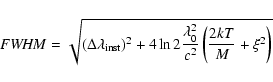
In Fig. 2 we plot the non-thermal velocities at three locations along the X-direction in the raster as shown in Fig. 1; i.e. position -133 $^{\prime\prime}$, -59 $^{\prime\prime}$ and +15 $^{\prime\prime}$, with the data being averaged over 21 pixels in X and 9 in Y. Here, we assume ionization equilibrium and that the ion temperature is identical to the electron temperature where the FWHM of the line is given by

$${\it FWHM} = \sqrt{(\Delta\lambda_{\rm inst})^2 + 4\ln 2 \frac{\lambda_0^2}{c^2} \left( \frac{2kT}{M} + \xi^2 \right) }$$ (1)

$\Delta\lambda_{\rm inst}$ is the instrumental width, $\lambda_0$ is the unshifted wavelength, c the speed of light, k the Boltzmann constant, T the ion temperature, M the atomic mass and $\xi$ the non-thermal velocity. The line was corrected for instrumental broadening using the SolarSoft routine: $CON\_WIDTH\_FUNCT\_3$.

Figure 3: A selection of spicules and macro-spicules showing the variation of the N  IV 765 Å intensity, non-thermal velocities and line-shift against height above the limb. The PCH was observed on 25 February 1997 between 00:03 and 13:58 UT. The times shown beside the curves are related to the starting time of the observation. Those at t=452 and 735 min are macro-spicules, while the others are spicules.

Open with DEXTER

In each plot, we clearly see a peak in the non-thermal velocity at $\approx$15 $^{\prime\prime}$ above the limb as seen in the continuum short-ward of O  V 629 Å. In the 450 and 500 plots, we see an additional broadening at $\approx$25-30 $^{\prime\prime}$. In order to gain some further insight into the nature of this off-limb broadening, we must look at the time series data. In Fig. 3 we show the velocity profiles (non-thermal and Doppler shift) derived from the N IV 765 Å line as a function of height above the limb. Despite the fact that N  IV is formed at around 140 000 K compared to O  V's 250 000 K, the non-thermal velocity variation is similar. It reaches maximum around 5 $^{\prime\prime}$ off-limb and remains at this value until around 18 $^{\prime\prime}$, shows a slight decrease before rising again around 25 $^{\prime\prime}$ off-limb.

Like the line radiance, the Doppler velocities are highly structured with a time scale down to 1 minute. Among them two examples (t=452 min and t=735 min) were identified as macro-spicules (Xia et al. 2005). Others (t=34, 261, 546, 630 min) are deduced as being "normal'' spicules.

In Fig. 3, one finds that the Doppler shifts of all selected structures are small (around $\pm$5  $\ {\rm km \; s}^{-1}$ or smaller) just above the limb, then quickly increases with height. After an initial acceleration, the velocity reaches a rather constant value, although with some fluctuation. The low velocity in this early stage of spicule evolution has also been found with CDS observations (Pike & Harrison 1997; Pike & Mason 1998). We suggest that the observed increase in the line broadening is not due to small scale motions but rather to unresolved line shifts due to spicules around 10 to 15 $^{\prime\prime}$, and then macro-spicules further off-limb.

Figure 4 shows a plot of the non-thermal velocity above the limb, taken from a region without obvious spicules (dotted line) and the whole observed data averaged (solid line). The solid line is the non-thermal velocity averaged from all the data, i.e., the line profile at every Y pixel is averaged across the entire 794 time series, then getting the line parameter from this re-binned profile. The dotted line is the non-thermal velocity averaged across a dark region from 554 min to 557 min. Again, after getting an average line profile at every Y pixel, then the line width. The non-spicule region has a peak non-thermal velocity between 7 and 10 $^{\prime\prime}$ off-limb, and shows a significantly smaller non-thermal velocity above 10 $^{\prime\prime}$ off-limb than that from the spicule region.

Note that the non-thermal velocities shown in Figs. 3 and 4 (obtained by SUMER detector B) are systematically larger than those shown in Fig. 2 (obtained by the SUMER detector A). This is possibly because of an insufficient subtraction of the instrumental broadening of the detector B, as discussed by Popescu et al. (2004).

	Figure 4: A plot of non-thermal velocities above the limb, taken from a time-region without obvious spicules (dotted line) and the whole observed data averaged (solid line).
Open with DEXTER

4 Discussion

There are many suggestions for the excess broadening of transition region lines, e.g. acoustic waves, Alfvén waves, opacity, turbulence, etc. Dere (1989) showed that the power in unresolved velocity variations (from line width measurements) was greater than that predicted from the extrapolated power of the resolved velocity variations (from line shift measurements), therefore suggesting the unresolved motions could be driven by a process that is different from those producing the line shifts. The idea behind the present study was not to explain the general broadening in excess of the thermal width, but rather to explain the additional increase in broadening seen in transition region lines about 10 000 km above the limb. This seems to be confined to a region of $\sim$3000 km.

Tu & Marsch (1997) suggested that ion-cyclotron is an important process in the solar wind. Peter & Vocks (2003) have more recently suggested that ion-cyclotron could be a possible mechanism to explain this additional line broadening above the limb. Although this is an interesting idea, it is difficult to understand why it should be confined to such a small region. In the analysis of transition region lines, Chae et al. (1998) and Doyle et al. (2000) both noted a 2-3  $\ {\rm km \; s}^{-1}$ difference in the line width from disk center to the limb. This could be explained via an increase in opacity from zero at disk center to unity at the limb. Doyle & McWhirter (1980) showed many years ago that some transition region lines were slightly effected by opacity at the limb. However, to produce a 10 km s^-1 increase via opacity would imply unrealistic high optical depths. The above authors also showed that the center-to-limb increase in line width could be reproduced assuming the presence of mass flows with a most probable speed of 5 km s^-1.

The present results suggest that spicule flows could play a role in line broadening. Macro-spicules (assumed to be the large-scale version of spicules) come in two types; erupting loops and spiked-jets. Yamauchi et al. (2004) found that 43% are of the erupting-loop type while 49% were the single-column spiked jet. However, even the erupting-loop type produces two columns when the loop top rises and probably reconnects with open-field structures. The velocities of both types of macro-spicules are in the range 32 to 42  $\ {\rm km \; s}^{-1}$. It is expected that the velocities in spicules are smaller than these values. This is consistent with the observations that the spicules velocity just above the limb is small and quickly under-goes acceleration just above the limb. Tanaka (1972) found that 30% of H$\alpha$ spicules produced a double-column structure, hence adding an increasing amount of line shift. The spicule contribution to the line widths is confirmed in Fig. 4 which shows that the line width taken from a region without obvious spicules is substantially smaller above 10 $^{\prime\prime}$ than that from a region with spicules.

Acknowledgements

Research at the Armagh Observatory is grant-aided by the N. Ireland Dept. of Culture, Arts and Leisure. L.D.X. is grateful for a PRTLI research grant for Grid-enabled Computational Physics of Natural Phenomena (Cosmogrid) and J.G. to PPARC for funding via the Armagh Observatory's visitors grant PPA/V/S/1999/00628. This work was also supported in part by PPARC grant PPA/G/S/2002/00020. We thank Georgia Tsiropoula for valuable comments on an earlier draft.

References

• Banerjee, D., Teriaca, L., Doyle, J. G., & Wilhelm, K. 1998, A&A, 339, 208 [NASA ADS] (In the text)
• Chae, J., Schuhle, U., & Lemaire, P. 1998, ApJ, 505, 957 [NASA ADS] [CrossRef] (In the text)
• Dammasch, I. E., Wilhelm, K., Curdt, W., & Hassler, D. M. 1999, A&A, 346, 285 [NASA ADS] (In the text)
• Dere, K. P. 1989, ApJ, 340, 599 [NASA ADS] (In the text)
• Doyle, J. G., & McWhirter, R. W. P. 1980, MNRAS, 193, 947 [NASA ADS] (In the text)
• Doyle, J. G., Teriaca, L., & Banerjee, D. 1999, A&A, 349, 956 [NASA ADS] (In the text)
• Doyle, J. G., Teriaca, L., & Banerjee, D. 2000, A&A, 356, 335 [NASA ADS] (In the text)
• Erdelyi, R., Doyle, J. G., Perez, M. E., & Wilhelm, K. 1998, A&A, 337, 287 [NASA ADS] (In the text)
• Harrison, R. A., Hood, A. W., & Pike, C. D., A&A, 392, 319
• Lemaire, P., Wilhelm, K., Curdt, W., et al. 1997, Sol. Phys., 170, 105 [NASA ADS] [CrossRef] (In the text)
• Mariska, J. T., Feldman, U., & Doschek, G. A. 1979, A&A, 73, 361 [NASA ADS] (In the text)
• O'Shea, E., Banerjee, D., & Poedts, S. 2003, A&A, 400, 1065 [EDP Sciences] [NASA ADS] [CrossRef] (In the text)
• O'Shea, E., Banerjee, D., & Doyle, J. G. 2005, A&A, submitted (In the text)
• Peter, H., & Vocks, C. 2003, A&A, 411, L481 [EDP Sciences] [NASA ADS] (In the text)
• Pike, C. D., & Harrison, R. A. 1997, Sol. Phys., 175, 457 [NASA ADS] (In the text)
• Pike, C. D., & Mason, H. E. 1998, Sol. Phys., 182, 333 [NASA ADS] (In the text)
• Popescu, M. D., Doyle, J. G., & Xia, L. D. 2004, A&A, 421, 339 [EDP Sciences] [NASA ADS] (In the text)
• Tanaka, K. 1972, Big Bear Obs. Rep., 125 (In the text)
• Tu, C.-Y., & Marsch, E. 1997, Sol. Phys., 171, 363 [NASA ADS] (In the text)
• Wilhelm, K., Curdt, W., Marsch, E., et al. 1995, Sol. Phys., 162, 189 [NASA ADS] (In the text)
• Wilhelm, K., Lemaire, P., Curdt, W., et al. 1997, Sol. Phys., 170, 75 [NASA ADS] [CrossRef] (In the text)
• Xia, L. D. 2003, Ph.D. Thesis, Georg-August-Univ., Göttingen (In the text)
• Xia, L. D., Popescu, M. D., Doyle, J. G., & Giannikakis, J. 2005, A&A, submitted (In the text)
• Yamauchi, Y., Moore, R. L., Suess, S. T., Wang, H., & Sakurai, T. 2004, ApJ, 605, 511 [NASA ADS] (In the text)