S. Vaughan
X-Ray and Observational Astronomy Group, University of Leicester, Leicester, LE1 7RH, UK
Received 11 June 2004 / Accepted 12 October 2004
Abstract
We demonstrate a simple method for testing the significance of peaks
in the periodogram of red noise data. The procedure was designed to
test for spurious periodicities in X-ray light curves of active
galaxies, but can be used quite generally to test for periodic
components against a background noise spectrum assumed to have a power
law shape. The method provides a simple and fast test of the
significance of candidate periodic signals in short, well-sampled time
series such as those obtained from XMM-Newton observations of Seyfert
galaxies, without the need for Monte Carlo simulations.
A full account is made of the number of trials and the
uncertainties inherent to the model fitting. Ignoring
these subtle effects can lead to substantially overestimated
significances. These difficulties motivate us to
demand high standards of detection (minimum >99.9 per cent confidence) for
periodicities in sources that normally show red noise spectra.
The method also provides a simple means to estimate the power spectral index, which may
be an interesting parameter itself, regardless of the presence/absence of
periodicities.
Key words: methods: data analysis - methods: statistical - X-rays: general - X-rays: galaxies
Many astrophysical sources show erratic, aperiodic brightness fluctuations with steep power spectra. This type of variability is known as red noise. By "noise'' we mean to say that the intrinsic variations in the source brightness are random (this has nothing to do with measurement errors, also called noise). Examples include the X-ray variability of X-ray binaries (XRBs; e.g. van der Klis 1995) and Seyfert galaxies (e.g. Lawrence et al. 1987; Markowitz et al. 2003). The power spectrum of these variations, which describes the dependence of the variability amplitude on temporal frequency, is often reasonably approximated as a simple power law (over at least a decade of frequency). This featureless continuum spectrum does not offer any characteristic frequencies that could be used as diagnostics.
XRBs often show quasi-periodic oscillations (QPOs) that show-up as
peaks in the power spectrum over the continuum noise spectrum. These
can be thought of as half-way between strictly periodic variations (all power concentrated at one
frequency) and broad-band noise (power spread over a very broad range
of frequencies). A combination of periodic oscillations with similar
frequencies, or a single oscillation that is perturbed in frequency,
amplitude or phase can produce a QPO. QPOs are one of
the most powerful diagnostics of XRB physics (see e.g. van der Klis
1995; M![]() Clintock & Remillard 2004).
The detection of periodic or quasi-periodic variations from a Seyfert galaxy would a be a key
observational discovery, and could lead to a breakthrough in our
understanding if the characteristic (peak) frequency could be
identified with some physically meaningful frequency.
For example, if we assume a
Clintock & Remillard 2004).
The detection of periodic or quasi-periodic variations from a Seyfert galaxy would a be a key
observational discovery, and could lead to a breakthrough in our
understanding if the characteristic (peak) frequency could be
identified with some physically meaningful frequency.
For example, if we assume a
![]() scaling of frequencies we might expect to see
analogues of the high frequency QPOs of XRBs in the range
scaling of frequencies we might expect to see
analogues of the high frequency QPOs of XRBs in the range
![]()
![]()
![]() Hz
(Abramowicz et al. 2004).
Hz
(Abramowicz et al. 2004).
However, claims of periodic variations and QPOs in the X-ray emission of Seyfert galaxies have a chequered history, with no single example withstanding the test of repeated analyses and observations (see discussion in Benlloch et al. 2001). The confusion arises partly due to the lack of a standard technique to assess the significance of a periodicity claim against a background assumption of random, red noise variability. Indeed, as Press (1978) and others have remarked, there is a tendency for the eye to identify spurious, low frequency periods in random time series. Tests for the presence of periodic variations against a background of white (flat spectrum) noise are well established, from Schuster (1898) and Fisher (1929), these are reviewed in Sect. 6.1.4 of Priestley (1981), and discussed in an astrophysical context by Leahy et al. (1983) and van der Klis (1989). But without modification these methods cannot be used to test against red noise variations. Timmer & König (1995) and Benlloch et al. (2001) have proposed Monte Carlo testing methods applicable to red noise but the relatively high computational demands of these methods may be enough to deter some potential users. Israel & Stella (1996) proposed a method that does not require Monte Carlo simulations but is not optimised for short observations of power law continuum spectra.
This paper puts forward a simple test that can be used to test the significance of candidate periodicities superposed on a red noise spectrum which has an approximately power law shape. The price of simplicity, in this case, is that the test is only strictly valid when the underlying continuum spectrum is a power law. The basic steps of the method are: (i) measure the periodogram; (ii) estimate the red noise continuum spectrum; and (iii) estimate the significance of any peaks above the continuum. The stages of the method are explained in detail in the following sections. Section 2 gives a brief introduction to the statistical properties of the periodogram. Section 3 discusses a simple method for estimating the parameters of a power law-like spectrum and Sect. 4 discusses how to estimate the significance of a peak above the continuum. Section 5 then demonstrates the veracity of the method using Monte Carlo simulations and Sect. 6 reviews some important caveats that must be considered when using this (and other) period-searching methods. Finally, Sect. 7 gives a brief review of the method in the context of observations of active galaxies. The appendix discusses a more generally applicable method of periodogram fitting (that makes no assumption on the form of the underlying spectrum).
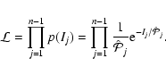
Given an evenly sampled time series xk of K points sampled at
intervals ![]() we can measure its periodogram (Schuster 1898), which is simply the
modulus-squared of the discrete Fourier transform, X(fj), at each
of the n=K/2 Fourier frequencies:
we can measure its periodogram (Schuster 1898), which is simply the
modulus-squared of the discrete Fourier transform, X(fj), at each
of the n=K/2 Fourier frequencies:
If the spectrum is flat ("white noise'') and its power level known a priori then we can simply make use of the known probability distribution (Eqs. (2) and (3)) to estimate the likelihood that a given periodogram ordinate exceeds some threshold. If the power level is not known there is an added uncertainty, but nevertheless an exact test does exist (Fisher's g statistic: Fisher 1929; Sect. 6.1.4 of Priestley 1981) to estimate the likelihood that the highest peak in the periodogram was caused by a random fluctuation in the noise spectrum (see also Koen 1990).
For the more general case of non-white noise there is no such exact
test. When examining the periodogram of red noise data such as from
Seyfert galaxies, we need to be careful not to identify spurious
peaks. Even in the "null'' case (i.e. no periodic component) peaks
may occur in the periodogram due to sampling fluctuations. In
particular the eye may be drawn to low frequency peaks because, in red
noise data, there is much more power and more scatter in the
periodogram at low frequencies. Given a large amount of data we can
average the periodogram in one of the standard ways (see e.g. van der Klis 1989; Papadakis & Lawrence 1993a), fit the continuum using a standard ![]() -minimisation tool (e.g. Bevington & Robinson 1992; Press et al. 1996) and test of the
presence of addition features. This is the standard procedure for
analysing XRB data. If we have a very limited amount of data, such
that we cannot afford to average the periodogram, we are faced with a
more difficult situation. Figure 1 gives an
example like this. The periodogram of a short time series, containing
red noise (generated using the method of Timmer & König
1995), shows a large peak at f=4
-minimisation tool (e.g. Bevington & Robinson 1992; Press et al. 1996) and test of the
presence of addition features. This is the standard procedure for
analysing XRB data. If we have a very limited amount of data, such
that we cannot afford to average the periodogram, we are faced with a
more difficult situation. Figure 1 gives an
example like this. The periodogram of a short time series, containing
red noise (generated using the method of Timmer & König
1995), shows a large peak at f=4 ![]() 10-2. Could this be
due to a real periodic variation present in the data or is it just a
fluctuation in the red noise spectrum?
10-2. Could this be
due to a real periodic variation present in the data or is it just a
fluctuation in the red noise spectrum?
![\begin{figure}
\par\includegraphics[angle=270,width=7.75cm,clip]{1453fig1.ps}\end{figure}](/articles/aa/full/2005/07/aa1453/img25.gif) |
Figure 1:
Periodogram of a short (K=256) time series containing red noise.
The upper panel shows the periodogram using linear axes,
the lower panel shows the same data on logarithmic axes.
The periodogram shows a red noise spectrum
rising at lower frequencies. But the periodogram also
shows a peak at f=4 |
| Open with DEXTER | |
If the underlying power spectrum is suspected to be a power law then
the parameters of interest are its slope, ![]() ,
and normalisation N. One of the simplest methods to estimate these parameters from the raw (unbinned) periodogram is to fit it with a model of the form
,
and normalisation N. One of the simplest methods to estimate these parameters from the raw (unbinned) periodogram is to fit it with a model of the form
![]() using the method of least squares (LS). The
problem with this is that the periodogram is distributed around the true underlying spectrum in a non-Gaussian fashion and, more seriously, the distribution depends on the spectrum itself
(Eq. (2)).
using the method of least squares (LS). The
problem with this is that the periodogram is distributed around the true underlying spectrum in a non-Gaussian fashion and, more seriously, the distribution depends on the spectrum itself
(Eq. (2)).
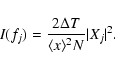
To simplify the problem we can fit the logarithm of
the periodogram, as discussed in some detail by Geweke & Porter-Hudak (1983; see also Papadakis & Lawrence 1993a). The scatter in the periodogram scales with the spectrum itself; the scatter is multiplicative in linear-space. This means the scatter is additive
in log-space:
![\begin{displaymath}%
\log\left[I\left(f_j\right)\right] = \log\left[\mathcal{P}\left(f_j\right)\right] + \log\left[ \chi_{2}^{2}/2\right]
\end{displaymath}](/articles/aa/full/2005/07/aa1453/img28.gif) |
(4) |
We must be careful fitting the logarithm. The expectation value of
the logarithm of the periodogram is not the expectation value
of the logarithm of the spectrum. However, the bias is a constant (due
to the shape of the
![]() -distribution in log-space) that can
be removed trivially:
-distribution in log-space) that can
be removed trivially:
![\begin{displaymath}%
\left\langle \log\left[I\left(f_j\right)\right] \right\rang...
...+ \left\langle \log\left[ \chi_{2}^{2}/2\right] \right\rangle.
\end{displaymath}](/articles/aa/full/2005/07/aa1453/img30.gif) |
(5) |
![\begin{displaymath}%
\left\langle \log\left[\mathcal{P}\left(f_j\right)\right] \...
...log\left[I\left(f_j\right)\right]\right\rangle
+0.25068 \ldots
\end{displaymath}](/articles/aa/full/2005/07/aa1453/img32.gif) |
(6) |
It is important to note that the datum at the Nyquist frequency (j=n) should be ignored in the LS fitting. This is because, as mentioned previously, the distribution of the periodogram ordinate
at this frequency is not identical to that at other frequencies (it follows
a ![]() distribution). This minor detail means that the
LS fit should be performed on the
distribution). This minor detail means that the
LS fit should be performed on the
![]() lowest frequencies
that are identically distributed (in log-space).
lowest frequencies
that are identically distributed (in log-space).
A drawback of fitting the periodogram, rather than the binned or averaged periodogram, is that it does not provide a in-built goodness-of-fit test. By binning
the periodogram (van der Klis 1989; Papadakis & Lawrence 1993a) we can obtain Gaussian errors on each ordinate to be used in a ![]() -test. We do not have Gaussian error bars for
the unbinned log-periodogram. But, since we know the expected distribution
of the periodogram ordinates about the true spectrum we can
compare this to the distribution of residuals from the fitted
data using a Kolmogorov-Smirnov test (Press et al. 1996).
Specifically, we can compare the data/model ratio (in linear space)
given by
-test. We do not have Gaussian error bars for
the unbinned log-periodogram. But, since we know the expected distribution
of the periodogram ordinates about the true spectrum we can
compare this to the distribution of residuals from the fitted
data using a Kolmogorov-Smirnov test (Press et al. 1996).
Specifically, we can compare the data/model ratio (in linear space)
given by
![]() with the theoretical
with the theoretical ![]() distribution, if the model is
reasonable
distribution, if the model is
reasonable
![]() should be consistent with the
should be consistent with the ![]() distribution. Furthermore, the KS test is most sensitive around the median value, and less sensitive at the tails of the distribution, which means that even in the presence of a real periodic signals
(i.e. a few outlying powers) the test should give a good idea of the overall quality of the
continuum fit.
distribution. Furthermore, the KS test is most sensitive around the median value, and less sensitive at the tails of the distribution, which means that even in the presence of a real periodic signals
(i.e. a few outlying powers) the test should give a good idea of the overall quality of the
continuum fit.
![\begin{figure}
\par\includegraphics[angle=270,width=8.15cm,clip]{1453f2a.ps}\par...
...ace*{3mm}
\includegraphics[angle=270,width=8.15cm,clip]{1453f2b.ps}\end{figure}](/articles/aa/full/2005/07/aa1453/img44.gif) |
Figure 2:
Distribution of the slope and normalisation estimators derived from
105 Monte Carlo simulations of K=256 point time series (histogram). The "true'' spectral parameters were |
| Open with DEXTER | |
The uncertainties on the slope and normalisation estimates from
the LS method can be derived using the standard theory of linear regression
(e.g. Bevington & Robinson 1992; Press et al. 1996).
The error on the slope (index) and intercept (log normalisation) are:
 |
(9) |
The accuracy of these equations was tested using a Monte Carlo simulations. An
ensemble of random time series, each of length K, was generated
(using the method of Timmer & König 1995). For each series
the power spectral slope and normalisation were estimated using the
LS method discussed above. Figure 2 shows the distribution of
estimates for 105 realisations of time series
generated by a process with an
![]() spectrum. With only
n=127 periodogram points (i.e. K=256) the distribution of the estimates is
reasonably close to Gaussian. (The distribution of
spectrum. With only
n=127 periodogram points (i.e. K=256) the distribution of the estimates is
reasonably close to Gaussian. (The distribution of ![]() is log-normal because the estimated
quantity
is log-normal because the estimated
quantity
![]() is normally distributed in the LS fitting.)
These two parameters are covariant in the fit; a low estimate of the
slope tends to be correlated with a high estimate of the normalisation.
Figure 3 illustrates the covariance between the
two estimated parameters. The shape of these distributions is independent of the
spectral slope, this was confirmed using Monte Carlo simulations of spectra
with slopes in the range
is normally distributed in the LS fitting.)
These two parameters are covariant in the fit; a low estimate of the
slope tends to be correlated with a high estimate of the normalisation.
Figure 3 illustrates the covariance between the
two estimated parameters. The shape of these distributions is independent of the
spectral slope, this was confirmed using Monte Carlo simulations of spectra
with slopes in the range
![]() .
.
![\begin{figure}
\par\includegraphics[angle=270,width=8.1cm,clip]{1453fig3.ps}\end{figure}](/articles/aa/full/2005/07/aa1453/img55.gif) |
Figure 3:
Demonstration of the covariance in the estimates of slope and normalisation from
from LS fitting to the logarithm of the periodogram. The plot shows the results of fitting 5000
Monte Carlo simulations of an |
| Open with DEXTER | |
The uncertainties on
![]() and
and
![]() ,
and their
covariance, were estimated for different length series by the same Monte Carlo method as discussed above. These Monte Carlo uncertainties compare well with the theoretically
expected uncertainties for the LS fitting method as discussed above
(Fig. 4).
,
and their
covariance, were estimated for different length series by the same Monte Carlo method as discussed above. These Monte Carlo uncertainties compare well with the theoretically
expected uncertainties for the LS fitting method as discussed above
(Fig. 4).
![\begin{figure}
\par\includegraphics[width=8cm,clip]{1453fig4.ps}\end{figure}](/articles/aa/full/2005/07/aa1453/img57.gif) |
Figure 4:
Demonstration of the uncertainties from LS fitting to the logarithm of the periodogram.
For each value of K, 105 time series were simulated (with an |
| Open with DEXTER | |
The expected uncertainties and covariance of the two model parameters
can be combined to give an estimate of the uncertainty
of the logarithm of the model,
![]() ,
at a
frequency fj, using the standard error propagation formula.
,
at a
frequency fj, using the standard error propagation formula.
The distribution of the power in the model (in log-space),
![]() ,
is expected to be Gaussian with a width determined by the formula above. In linear-space the
uncertainty on the model power,
,
is expected to be Gaussian with a width determined by the formula above. In linear-space the
uncertainty on the model power,
![]() ,
is
log-normally distributed. The probability density function (PDF) for
the model power is therefore
,
is
log-normally distributed. The probability density function (PDF) for
the model power is therefore
![\begin{figure}
\par\includegraphics[angle=270,width=7.8cm,clip]{1453fig5.ps}\end{figure}](/articles/aa/full/2005/07/aa1453/img68.gif) |
Figure 5:
Monte Carlo demonstration of the distribution of power in the model (power law) spectrum.
Using an |
| Open with DEXTER | |
Although in general the LS method does not yield the maximum likelihood solution for non-Gaussian data, for the specific case of a power law spectrum the
parameters obtained from the log-periodogram regression,
namely
![]() and
and
![]() ,
are unbiased. Figure 6 demonstrates this using Monte Carlo simulations. However, it should be noted that because the
parameter
,
are unbiased. Figure 6 demonstrates this using Monte Carlo simulations. However, it should be noted that because the
parameter
![]() is normally distributed the parameter
is normally distributed the parameter ![]() will be log-normally distributed. Thus the mean value of
will be log-normally distributed. Thus the mean value of ![]() is not a good estimator of the true value (it will be
biased upwards due to the long tail of the log-normal distribution).
is not a good estimator of the true value (it will be
biased upwards due to the long tail of the log-normal distribution).
![\begin{figure}
\par\includegraphics[width=8cm,clip]{1453fig6.ps}\end{figure}](/articles/aa/full/2005/07/aa1453/img69.gif) |
Figure 6:
Demonstration of bias in LS fitting of the logarithm of the periodogram.
For each value of K, 105 time series were simulated (with an |
| Open with DEXTER | |
The following summarises the LS fitting method:
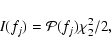
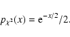
If we know the exact form of the spectrum we can divide this out of the periodogram. From Eq. (2) we can see that the ratio
![]() will be distributed like
will be distributed like ![]() .
We can use our estimates
.
We can use our estimates
![]() and
and ![]() to form the null hypothesis: the data were generated by a process with a spectrum
to form the null hypothesis: the data were generated by a process with a spectrum
![]() and no periodic component.
We can estimate the probability that a large peak will occur in the periodogram, assuming the model spectrum, by comparing
and no periodic component.
We can estimate the probability that a large peak will occur in the periodogram, assuming the model spectrum, by comparing
![]() to the
to the ![]() PDF (Priestley 1981; Scargle 1982).
PDF (Priestley 1981; Scargle 1982).
We can define a
![]() per cent confidence limit on
per cent confidence limit on
![]() ,
call this
,
call this
![]() ,
as the level for which, at a given frequency, the
probability of obtaining a higher value by chance is
,
as the level for which, at a given frequency, the
probability of obtaining a higher value by chance is
![]() on the assumption that the null hypothesis is
true. The chosen value of
on the assumption that the null hypothesis is
true. The chosen value of ![]() represents the "false alarm probability''.
The integral of the
represents the "false alarm probability''.
The integral of the ![]() probability density gives the probability of a single sample exceeding a value of
probability density gives the probability of a single sample exceeding a value of
![]() by chance:
by chance:
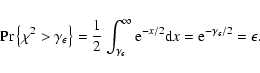 |
(14) |
However, these confidence bounds correspond to a single trial
test, they give the probability that a periodogram point at one particular
frequency will exceed
![]() .
Usually there are
.
Usually there are
![]() independent trials since only the Nyquist frequency is ignored (leaving
independent trials since only the Nyquist frequency is ignored (leaving
![]() independently distributed periodogram points to be examined).
We must account for the number of independent trials:
independently distributed periodogram points to be examined).
We must account for the number of independent trials:
The case outlined above is valid only when we know the true power
spectrum exactly (
![]() ).
In reality all we have is an estimated model
).
In reality all we have is an estimated model
![]() (which will differ from
the true spectrum) and its uncertainty. This extra
uncertainty alters the probability distribution. The ratio
(which will differ from
the true spectrum) and its uncertainty. This extra
uncertainty alters the probability distribution. The ratio
![]() is really the ratio of two random
variables; the PDF of this would allow us to calculate the probability
of observing a given value of
is really the ratio of two random
variables; the PDF of this would allow us to calculate the probability
of observing a given value of
![]() taking full account of
the uncertainty in the model fitting. As discussed above 2Ij will
follow a rescaled
taking full account of
the uncertainty in the model fitting. As discussed above 2Ij will
follow a rescaled ![]() distribution about the true spectrum.
distribution about the true spectrum.
 |
(17) |
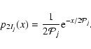
![\begin{displaymath}%
p_{\hat{\mathcal{P}}_j}(y) = \frac{1}{S_j y \sqrt{2 \pi}}
...
... \left\{ - \frac{\left(\ln[y] - M_j\right)^2}{2S_j^2} \right\}
\end{displaymath}](/articles/aa/full/2005/07/aa1453/img65.gif) |
(18) |
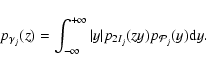
The PDF of the ratio
![]() can be obtained using the standard formula for the PDF
of the ratio of two independent variables:
can be obtained using the standard formula for the PDF
of the ratio of two independent variables:
 |
(19) |
For a given frequency fj the integral in Eq. (21) can be evaluated
numerically to give the PDF for
![]() .
Figure 7 compares the prediction of
Eq. (21) with a Monte Carlo distribution
at two different frequencies. Also shown for comparison is the
.
Figure 7 compares the prediction of
Eq. (21) with a Monte Carlo distribution
at two different frequencies. Also shown for comparison is the ![]() PDF which represents
the distribution in the absence of uncertainties on the model (i.e.
PDF which represents
the distribution in the absence of uncertainties on the model (i.e.
![]() ).
At small
).
At small
![]() (i.e. low significance peaks)
the two distributions agree, whereas for large
(i.e. low significance peaks)
the two distributions agree, whereas for large
![]() (i.e. high significance
peaks) there is a substantial difference between the PDFs including and
excluding the uncertainty on the model. This means that,
while the effect of including the uncertainty on the model is
negligible for low significance peaks, the significance of high
significance peaks may be substantially overestimated
if this additional uncertainty is not taken into account.
(i.e. high significance
peaks) there is a substantial difference between the PDFs including and
excluding the uncertainty on the model. This means that,
while the effect of including the uncertainty on the model is
negligible for low significance peaks, the significance of high
significance peaks may be substantially overestimated
if this additional uncertainty is not taken into account.
![\begin{figure}
\par\includegraphics[width=8cm,clip]{1453fig7.ps}\end{figure}](/articles/aa/full/2005/07/aa1453/img98.gif) |
Figure 7:
Monte Carlo demonstration of the PDF of the ratio
|
| Open with DEXTER | |
The probability of obtaining a value of
![]() higher
than
higher
than
![]() can be computed by integrating this PDF:
can be computed by integrating this PDF:
Finally, we need to correct for the number of frequencies examined.
The probability that a peak will be seen given that
![]() frequencies were examined is
frequencies were examined is
![]() .
One can find the global
.
One can find the global
![]() per cent
confidence level by finding the value
per cent
confidence level by finding the value
![]() that satisfies:
that satisfies:
As an illustration of the effect of the model uncertainty, consider a
peak in the j=10 frequency bin of a n=128 periodogram. Neglecting the effect of model uncertainty the nominal
![]() threshold is
threshold is
![]() (using
Eq. (15)). But, after including the uncertainty in the model,
the probability of this level being
exceeded is really 3.6
(using
Eq. (15)). But, after including the uncertainty in the model,
the probability of this level being
exceeded is really 3.6 ![]() 10-4 (using Eq. (22)).
For n=128 trials this corresponds to global significances of 98.7 per cent confidence (ignoring the model uncertainty) and 95.4 per cent confidence (including the model
uncertainty). The first of these might be called a significant
detection, but once the model uncertainty is taken into account
the detection is no longer very significant. The difference
is even more profound for higher significances.
10-4 (using Eq. (22)).
For n=128 trials this corresponds to global significances of 98.7 per cent confidence (ignoring the model uncertainty) and 95.4 per cent confidence (including the model
uncertainty). The first of these might be called a significant
detection, but once the model uncertainty is taken into account
the detection is no longer very significant. The difference
is even more profound for higher significances.
![\begin{figure}
\par\includegraphics[angle=270,width=8.15cm,clip]{1453f8a.ps}\par...
...ace*{3mm}
\includegraphics[angle=270,width=8.15cm,clip]{1453f8b.ps}\end{figure}](/articles/aa/full/2005/07/aa1453/img109.gif) |
Figure 8:
Monte Carlo study of the performance of tests for significant
periodogram peaks. For each panel 106 random time series
of length K=256 were generated (with an
|
| Open with DEXTER | |
The procedures discussed above were tested using Monte Carlo
simulations. The simulations measured the type I error rate, or
the rate of "false positive'' (spurious) detections of periodic signals.
For this experiment many artificial time series were generated based on a power law
spectrum (i.e. the null hypothesis). For each simulation the
![]() threshold, corresponding to a
threshold, corresponding to a
![]() confidence level, was calculated and the number of periodogram ordinates that exceeded this value were recorded.
The rate measured from the Monte Carlo simulations should be
the same as the false alarm probability
confidence level, was calculated and the number of periodogram ordinates that exceeded this value were recorded.
The rate measured from the Monte Carlo simulations should be
the same as the false alarm probability ![]() ,
often called the
"size of the test'', which is the expected rate of type I errors.
If the observed rate of false detections
exceeds the nominal size of the test then one should expect an
excess of spurious detections (detections may not be reliable). If the
observed rate falls below the nominal test size then the test is
conservative (it gives even fewer spurious detections than expected).
,
often called the
"size of the test'', which is the expected rate of type I errors.
If the observed rate of false detections
exceeds the nominal size of the test then one should expect an
excess of spurious detections (detections may not be reliable). If the
observed rate falls below the nominal test size then the test is
conservative (it gives even fewer spurious detections than expected).
The Monte Carlo rate was derived from 106 random time series of
length K=256 (generated with a
![]() spectrum). For each
series the periodogram was computed and fitted using the LS method.
In the first run, the effects of the uncertainty on the model were
ignored and the
spectrum). For each
series the periodogram was computed and fitted using the LS method.
In the first run, the effects of the uncertainty on the model were
ignored and the
![]() thresholds were computed for
thresholds were computed for
![]() and 10-4 using Eq. (15).
These corresponds to 99.9 and 99.99 per cent confidence levels
in a single trial test. For each frequency the fraction of simulations that
show peaks larger than the threshold was recorded. As shown in
Fig. 8 (upper panel) the observed rate of type I
errors in the simulated data was far in excess of the nominal size of the test.
Thus the actual rate of spurious detections was higher than
the nominal test size, and greatly so at low frequencies where the
model is more uncertain. The situation is worse at high significances
(small test sizes) because the tail of the PDF diverges from the
expectation (Fig. 7). This means that significances
calculated by Eq. (15) will be overestimated.
and 10-4 using Eq. (15).
These corresponds to 99.9 and 99.99 per cent confidence levels
in a single trial test. For each frequency the fraction of simulations that
show peaks larger than the threshold was recorded. As shown in
Fig. 8 (upper panel) the observed rate of type I
errors in the simulated data was far in excess of the nominal size of the test.
Thus the actual rate of spurious detections was higher than
the nominal test size, and greatly so at low frequencies where the
model is more uncertain. The situation is worse at high significances
(small test sizes) because the tail of the PDF diverges from the
expectation (Fig. 7). This means that significances
calculated by Eq. (15) will be overestimated.
The situation is much better when the
![]() threshold
was computed (again for
threshold
was computed (again for
![]() )
using
Eq. (22). Again 106 random time series were
generated with K=256 using the same spectrum. For each periodogram
the model power
)
using
Eq. (22). Again 106 random time series were
generated with K=256 using the same spectrum. For each periodogram
the model power
![]() ,
and its error parameters Sj,
were computed by ignoring frequency fj and then fitting with the LS method. The ratio
,
and its error parameters Sj,
were computed by ignoring frequency fj and then fitting with the LS method. The ratio
![]() was compared to the critical threshold
was compared to the critical threshold
![]() (computed from
Eq. (22)) at each frequency. The fraction of Monte Carlo
simulations that showed "significant'' peaks was very close
to the expected level (the nominal size) and independent of
frequency. The exceptions are the
(computed from
Eq. (22)) at each frequency. The fraction of Monte Carlo
simulations that showed "significant'' peaks was very close
to the expected level (the nominal size) and independent of
frequency. The exceptions are the ![]() 5 lowest frequencies.
Here the model is least constrained and the assumption
implicit in Eq. (11), that the distribution
of
5 lowest frequencies.
Here the model is least constrained and the assumption
implicit in Eq. (11), that the distribution
of
![]() is normal, becomes inaccurate.
For
is normal, becomes inaccurate.
For ![]() the confidence levels predicted by
Eq. (22) gave the correct rate of type I errors.
the confidence levels predicted by
Eq. (22) gave the correct rate of type I errors.
Figure 9 shows a specific example, namely the
same data as in Fig. 1, with the LS power law model.
Also shown are the ("global'')
![]() -trial confidence limits
computed as discussed in Sect. 4.2.
Clearly none of the peaks in the periodogram exceeds the
95 per cent limit, as expected for red noise.
-trial confidence limits
computed as discussed in Sect. 4.2.
Clearly none of the peaks in the periodogram exceeds the
95 per cent limit, as expected for red noise.
![\begin{figure}
\par\includegraphics[angle=270,width=8.35cm,clip]{1453fig9.ps}\end{figure}](/articles/aa/full/2005/07/aa1453/img115.gif) |
Figure 9: Same periodogram as in Fig. 1. Plotted are the de-biased LS estimate of the power law spectral model (solid curve) and the 95 and 99 per cent upper limits (dotted curves) on the expected power (global significance levels for n=127 independent frequencies). |
| Open with DEXTER | |
In order for the test to give reliable significance limits the
underlying noise spectrum must be a power law. Clearly if the
broad-band noise spectrum does not resemble a power law the results of
the LS fitting will not be valid. The general solution to this
problem is to replace the LS fitting procedure with the exact
maximum likelihood (ML) procedure for fitting the ![]() distributed
periodogram. The appendix describes this method.
distributed
periodogram. The appendix describes this method.
The test was intended to be used for assessing the significance of
peaks in the periodograms of X-ray observations of Seyfert galaxies,
which tend to be rather short
![]() and also show significant
variance due to measurement errors (Poisson noise). These measurement
uncertainties produce a flat component that is added to the source
power spectrum in the periodogram. The effect will cause the
observed spectrum to flatten at high frequencies as the power in the
red noise spectrum of the source becomes comparable to the power in
the flat Poisson noise spectrum. Using the normalisation given in
Eq. (1) the expected Poisson noise level is
and also show significant
variance due to measurement errors (Poisson noise). These measurement
uncertainties produce a flat component that is added to the source
power spectrum in the periodogram. The effect will cause the
observed spectrum to flatten at high frequencies as the power in the
red noise spectrum of the source becomes comparable to the power in
the flat Poisson noise spectrum. Using the normalisation given in
Eq. (1) the expected Poisson noise level is
![]() where
where
![]() is the mean count rate and B is the mean background rate
is the mean count rate and B is the mean background rate![]() .
It is also now known that at low frequencies the power spectra
of Seyferts break from a single power law (e.g. Uttley et al. 2002;
Markowitz et al. 2003). These deviations from a single power law
should be accounted for in modelling the spectrum.
The simplest solution is to divide the periodogram into
frequency ranges within which the power spectrum is approximately
a single power law. The period detection test can then be used
as described above. The crucial point is that as long as the periodogram can be fitted
reasonably well with a power law over a frequency
range of interest (as judged using the KS test) the test will be valid.
Alternatively one may fit a model of a power law plus
constant (to account for the flattening) using the ML method discussed in the Appendix.
.
It is also now known that at low frequencies the power spectra
of Seyferts break from a single power law (e.g. Uttley et al. 2002;
Markowitz et al. 2003). These deviations from a single power law
should be accounted for in modelling the spectrum.
The simplest solution is to divide the periodogram into
frequency ranges within which the power spectrum is approximately
a single power law. The period detection test can then be used
as described above. The crucial point is that as long as the periodogram can be fitted
reasonably well with a power law over a frequency
range of interest (as judged using the KS test) the test will be valid.
Alternatively one may fit a model of a power law plus
constant (to account for the flattening) using the ML method discussed in the Appendix.
Furthermore, the test, which is based on the discrete Fourier transform, is most sensitive to sinusoidal periodicities. Non-sinusoidal variations will have their power spread over several frequencies which will lessen the detection significance in any one given frequency. Other methods such as epoch folding (Leahy et al. 1983), whereby one bins the time series into phase bins at a test period, can be more sensitive to such variations. At the correct period the periodic variations will sum while any background noise will cancel out, thus revealing the profile of the periodic pulsations. However, the background noise will only cancel out if it is temporally independent, i.e. white noise. Again, the presence of any underlying red noise variations may produce unreliable results (Benlloch et al. 2001) if not correctly accounted.
The method described above is based around the standard (Fourier) periodogram and therefore requires uniformly sampled time series. This ensures the asymptotic independence of the periodogram ordinates. If the time series is non-uniformly sampled one may use other periodogram estimators such as the Lomb-Scargle periodogram (Lomb 1976; Scargle 1982; Press & Rybicki 1989). However, the behaviour of these will not be identical to that discussed above. The above procedure should not be used on non-uniformly sampled time series (nor should the method discussed in Sect. 13.8 of Press et al. 1996 be used in the presence of non-white noise). Zhou & Sornette (2001) discuss the results of Monte Carlo tests on the distribution of peaks in the Lomb-Scargle periodogram for various types of processes.
Oversampling the periodogram, i.e. calculating periodogram
ordinates at frequencies between the normal Fourier frequencies,
is sometimes done in order to increase the sensitivity to weak
signals that lie at frequencies between two Fourier frequencies.
A periodic variation with a frequency nearly equidistant
between two adjacent Fourier frequencies, e.g. between fj and fj+1,
will have its power spread (almost entirely) between these two
frequencies, thus reducing the significance in any one frequency bin.
The reduction in power per bin can be as much as ![]()
![]() .
In these situations oversampling the periodogram by including additional
frequencies between fj and fj+1 can increase sensitivity
to the periodicity. However, it must also be noted that by
oversampling the periodogram one is testing more than K/2 frequencies,
allowing many more opportunities to find spurious peaks. The number of
trials increases above the usual n=K/2 case if the periodogram is
oversampled, although the effective number of independent trials does
not scale linearly with the oversampling factor because there is a fixed number (n) of
strictly independent frequencies (the Fourier frequencies).
.
In these situations oversampling the periodogram by including additional
frequencies between fj and fj+1 can increase sensitivity
to the periodicity. However, it must also be noted that by
oversampling the periodogram one is testing more than K/2 frequencies,
allowing many more opportunities to find spurious peaks. The number of
trials increases above the usual n=K/2 case if the periodogram is
oversampled, although the effective number of independent trials does
not scale linearly with the oversampling factor because there is a fixed number (n) of
strictly independent frequencies (the Fourier frequencies).
Oversampling the periodogram and assuming ![]() n trials will
tend to overestimate the significance of peaks in the periodogram.
This was demonstrated by Monte Carlo simulations (see
Fig. 10). For this demonstration 104 white noise time series (spectrum:
n trials will
tend to overestimate the significance of peaks in the periodogram.
This was demonstrated by Monte Carlo simulations (see
Fig. 10). For this demonstration 104 white noise time series (spectrum:
![]() )
were generated with length K=256 and for each one the periodogram
was calculated using both the standard Fourier frequencies
and also oversampling the frequency resolution by a factor 8.
The peak power in the periodogram of each of the simulated time series
was recorded. The distribution of peak powers is shown in
Fig. 10 for both the standard and the oversampled
periodograms. There is an obvious tendency for the oversampled
periodogram to show slightly higher peak values, as might be expected
based on the above arguments. These peak powers were translated to
"global'' significances (assuming n independent trials) and the
distribution of significances is shown in the lower panel of
Fig. 10. The distribution is flat
for the Fourier sampled periodogram: the significance of the peaks
is exactly as expected. The distribution derived from the oversampled
periodogram clearly shows a substantial excess of high significance
peaks. This means that the oversampled periodogram is likely to
produce many more spurious peaks than expected if one assumes only n independent trials were made. A Monte Carlo estimate of the global significance would be
required to calibrate the significance of peaks in oversampled
periodogram (and find a more realistic effective number of trials).
)
were generated with length K=256 and for each one the periodogram
was calculated using both the standard Fourier frequencies
and also oversampling the frequency resolution by a factor 8.
The peak power in the periodogram of each of the simulated time series
was recorded. The distribution of peak powers is shown in
Fig. 10 for both the standard and the oversampled
periodograms. There is an obvious tendency for the oversampled
periodogram to show slightly higher peak values, as might be expected
based on the above arguments. These peak powers were translated to
"global'' significances (assuming n independent trials) and the
distribution of significances is shown in the lower panel of
Fig. 10. The distribution is flat
for the Fourier sampled periodogram: the significance of the peaks
is exactly as expected. The distribution derived from the oversampled
periodogram clearly shows a substantial excess of high significance
peaks. This means that the oversampled periodogram is likely to
produce many more spurious peaks than expected if one assumes only n independent trials were made. A Monte Carlo estimate of the global significance would be
required to calibrate the significance of peaks in oversampled
periodogram (and find a more realistic effective number of trials).
![\begin{figure}
\par\includegraphics[angle=270,width=8.25cm,clip]{1453f10a.ps}\pa...
...ce*{3mm}
\includegraphics[angle=270,width=8.25cm,clip]{1453f10b.ps}\end{figure}](/articles/aa/full/2005/07/aa1453/img122.gif) |
Figure 10:
Comparison between periodograms sampled at the K/2 Fourier frequencies and oversampled by a factor 8. The upper panel shows the distribution of peaks in the periodogram from 104 random white noise time series of length K=256 (using an
|
| Open with DEXTER | |
An alternative to oversampling the periodogram is to perform a sliding two-bin search for periodogram peaks using the standard Fourier frequencies only, as discussed by van der Klis (1989; Sect. 6.4). This increases the sensitivity to periods whose frequencies fall between the Fourier frequencies. However, one will still need to perform Monte Carlo simulations to assess the global significance (by measuring the rate of type I errors in the simulations).
An alternative test for periodic variations in red noise is to estimate the likelihood of observing a given peak using Monte Carlo simulations of red noise processes (Benlloch et al. 2001; Halpern et al. 2003). However, the method of Benlloch et al. (2001) does not account for uncertainties in the best-fitting model, which can seriously effect the apparent significances of strong peaks (Sect. 4.2). Monte Carlo simulations are only as good as the model they assume! One solution would be to map the (multi-dimensional) distribution of the model parameters and for each simulation draw the model parameters at random from this distribution. This would thereby account for the uncertainty in the model parameters. (Protassov et al. 2002 use a similar approach to calculate posterior predictive p-values.)
A simple procedure is presented for assessing the significance of peaks in a periodogram when the underlying continuum noise has a power law spectrum.
The following is one possible recipe for periodogram analysis.
For a given frequency of interest, fj, one must:
In order for the method to produce reliable results the underlying power spectrum has to be a power law. However, the test will work well even for data that show deviations from a power law (such as intrinsic low frequency flattening or high frequency flattening due to Poisson noise) provided the periodogram is divided into frequency intervals within which a single power law provides a good description of the data (determined with a KS test). In this case the power spectrum over the restricted frequency ranges is indistinguishable from a power law and, when applied to these limited frequency ranges, the method will function as expected.
As a demonstration of the method we present a re-analysis of the X-ray observations of two Seyfert galaxies. The first is the long ASCA observation of IRAS 18325-5926 (Iwasawa et al. 1998) and the second is the XMM-Newton GTO observation of Mrk 766 (Boller et al. 2001). For IRAS 18325-5926 a background-subtracted 0.5-10 keV SIS0 light curve was extracted in 100-s bins, using a 4 arcmin radius source region, and rebinned onto an evenly spaced grid at the spacecraft orbital period (5760-s). For Mrk 766 a background-subtracted, exposure-corrected 0.2-2 keV light curve was extracted from the EPIC pn using a 38 arcsec radius source region. The rebinned IRAS 18325-5926 light curve contained 84 regularly spaced bins and the Mrk 766 light curve contained 330 contiguous 100-s bins.
The periodogram of each light curve was calculated and the expected
Poisson noise level determined. Only the
lowest frequency periodogram points were examined, to minimise the
effect of the Poisson noise level. For IRAS 18325-5926 only the 19 lowest frequency points were used, while for Mrk 766 only 97 points were used. These were fitted with a linear function in log-space, giving slopes of
![]() and
and
![]() for
IRAS 18325-5926 and Mrk 766, respectively. The 95 and 99 per cent confidence limits on the periodogram were computed, accounting for the number of frequencies examined in each case (see
Figs. 11 and 12). In neither object did a
single periodogram point exceed the 95 per cent limit, meaning that
there is no strong evidence to suggest a periodic component to their
variability, contrary to the original claims of Iwasawa et al. (1998;
for
IRAS 18325-5926 and Mrk 766, respectively. The 95 and 99 per cent confidence limits on the periodogram were computed, accounting for the number of frequencies examined in each case (see
Figs. 11 and 12). In neither object did a
single periodogram point exceed the 95 per cent limit, meaning that
there is no strong evidence to suggest a periodic component to their
variability, contrary to the original claims of Iwasawa et al. (1998;
![]()
![]() 10-5 Hz) and Boller et al. (2001;
10-5 Hz) and Boller et al. (2001;
![]()
![]() 10-4 Hz). Benlloch et al. (2001) drew similar conclusions
based on Monte Carlo simulations.
10-4 Hz). Benlloch et al. (2001) drew similar conclusions
based on Monte Carlo simulations.
![\begin{figure}
\par\includegraphics[angle=270,width=8.4cm,clip]{1453f11.ps}\end{figure}](/articles/aa/full/2005/07/aa1453/img130.gif) |
Figure 11: Periodogram of IRAS 18325-5926 from ASCA. Plotted are the de-biased LS estimate of the power law spectral model (solid curve) and the 95 and 99 per cent upper limits (dotted curves) on the expected power (global significance levels for n=19 independent frequencies). Also shown is the expected level of the Poisson noise power. |
| Open with DEXTER | |
![\begin{figure}
\par\includegraphics[angle=270,width=8.3cm,clip]{1453f12.ps}\end{figure}](/articles/aa/full/2005/07/aa1453/img131.gif) |
Figure 12: Periodogram of Mrk 766 from XMM-Newton. |
| Open with DEXTER | |
The simplicity of the proposed test means that it can be used as a quick, first check against spurious periodogram peaks, without the need for extensive Monte Carlo simulations. Examples where this test might be useful include not only X-ray observations of Seyferts but also testing for periodic components in monitoring of blazars (e.g. Kranich et al. 1999; Hayashida et al. 1998), the Galactic centre (Genzel et al. 2003) and other astrophysical sources that show red noise variations.
The basic idea behind the method is to de-redden the periodogram by dividing out the best-fitting power law and then using the known distribution of the periodogram ordinates to estimate the likelihood of observing a given peak if the null hypothesis (power law spectrum with no periodicity) is true. However, this should not be treated as a "black box'' solution to the problem of detecting periodicities in red noise data. There is no substitute for a thorough understanding of the nuances of power spectral statistics, as illustrated by the PDFs discussed in Sect. 4.2. The tail of the PDF is very sensitive to the details of the method, and thus one needs to treat any periodogram analysis with great care in order to avoid overestimating the significance of a peak.
To date the most significant candidate periodicities found in the X-ray variations active galaxies are those in long EUVE observations of three nearby Seyferts by Halpern et al. (2003). However, their published global significances will be overestimates for two reasons: (i) no account was made of the uncertainty on the model and (ii) the periodograms were oversampled. These two separate issues both act to artificially boost the apparent significance of spurious signals, as discussed in Sects. 4.2 and 6.2.2, respectively. Similarly the apparently significant candidate periodicity in NGC 5548 found by Papadakis & Lawrence (1993b) was shown to be substantially less significant when the uncertainty in the modelling was included (Tagliaferri et al. 1996). This leaves us in the interesting situation of there being not one surviving, robustly determined and significant (>99 per cent) periodicity in the X-ray variability of an active galaxy.
Finally we close with a plea. There exist many more AGN light curves
and periodograms than have been published. There is a natural
publication bias: those that show the most "significant'' features get
published. This means the true number
of trials is much larger than for any one given experiment. In such
situations one should treat
with caution the significance of the subset of results that are
published (e.g. Scargle 2000).
That is, until a result is published that is so significant
that it cannot be accounted for by publication bias. The detection
of periodic or quasi-periodic variations in galactic nuclei would be a
major discovery and of great importance to the field. The importance
of the result should be argument enough for very high standards of
discovery. We would therefore advocate serious further investigation of
only those candidate periodicities with high significances
(such as a >99.9 per cent confidence, or a "![]() minimum,''
criterion) after accounting for all likely sources of error.
minimum,''
criterion) after accounting for all likely sources of error.
Acknowledgements
I acknowledge financial support from the PPARC, UK. I also thank Phil Uttley for many useful discussions and Iossif Papadakis for a very thorough referee's report that encouraged me to expand several sections of the paper.
In this section we briefly elucidate the exact method of
maximum likelihood (ML) fitting periodograms. See Anderson, Duvall &
Jefferies (1990) and Stella et al. (1997) for more
details. The probability density function (PDF) of the periodogram ordinates
at each frequency are given by:
 |
(A.1) |
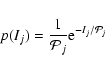
Assuming a model
![]() ,
determined by
parameters
,
determined by
parameters
![]() ,
we can write the joint
probability density of observing the n-1 periodogram ordinates:
,
we can write the joint
probability density of observing the n-1 periodogram ordinates:
 |
(A.2) |
![\begin{displaymath}%
S = 2 \sum_{j=1}^{n-1} \left\{ \ln\left[\hat{\mathcal{P}}_j\right] + \frac{I_j}{\hat{\mathcal{P}}_j} \right\}\cdot
\end{displaymath}](/articles/aa/full/2005/07/aa1453/img140.gif) |
(A.3) |
One can then use standard tools of maximum likelihood analysis,
such as the likelihood ratio test (LRT) to test for additional
free parameters in the model:
| (A.4) |
Alternatively one can compare different models using the Akaike
Information Criterion (AIC; Akaike 1973):
| (A.5) |
One can also use
![]() to place
confidence limits on the model parameters in a fashion exactly
analogous to mapping confidence contours using
to place
confidence limits on the model parameters in a fashion exactly
analogous to mapping confidence contours using
![]() (Sect. 15.6 of Press et al. 1996). Under fairly general conditions
(see Cash 1979), e.g. the
(Sect. 15.6 of Press et al. 1996). Under fairly general conditions
(see Cash 1979), e.g. the
![]() -surface is
approximately shaped like a multi-dimensional paraboloid,
-surface is
approximately shaped like a multi-dimensional paraboloid, ![]() is
distributed as
is
distributed as
![]() where
where ![]() is the number of
parameters of interest (e.g.
is the number of
parameters of interest (e.g. ![]() for the one-dimensional
confidence region on an individual parameter). One can use
standard tables of
for the one-dimensional
confidence region on an individual parameter). One can use
standard tables of
![]() values to place
confidence limits (e.g.
values to place
confidence limits (e.g.
![]() corresponds to 90 per cent
confidence limits on one parameter).
corresponds to 90 per cent
confidence limits on one parameter).
For the purposes of period searching one may fit a suitable
M-parameter continuum model (representing the null hypothesis, i.e.,
no periodic signal) using the ML method and define the
M-dimensional distribution of its parameters (using ![]() ). One can then use this M-dimensional distribution of the model parameters to randomly draw models for
Monte Carlo simulation. This procedure will thereby account for the
likely distribution of model parameters (which gives rise to
uncertainties in the estimated continuum level).
). One can then use this M-dimensional distribution of the model parameters to randomly draw models for
Monte Carlo simulation. This procedure will thereby account for the
likely distribution of model parameters (which gives rise to
uncertainties in the estimated continuum level).
![\begin{displaymath}%
{\rm err}^2 \left[ \hat{\alpha} \right] = \frac{n^{\prime} \sigma^2}{ \Delta }
\end{displaymath}](/articles/aa/full/2005/07/aa1453/img45.gif)
![\begin{displaymath}%
{\rm err}^2 \left[ \log\left(\hat{N}\right)\right] = \frac{ \sigma^2 \sum_{j=1}^{n^{\prime}} a_j^2 }{ \Delta }
\end{displaymath}](/articles/aa/full/2005/07/aa1453/img46.gif)
![\begin{displaymath}%
{\rm cov}\left[\hat{\alpha},\log\left(\hat{N}\right)\right] = \frac{ \sigma^2 \sum_{j=1}^{n^{\prime}} a_j }{ \Delta }\cdot
\end{displaymath}](/articles/aa/full/2005/07/aa1453/img50.gif)
![\begin{displaymath}%
S_j = {\rm err}\left[ \log \left\{ \hat{\mathcal{P}}\left(f_j\right) \right\} \right] \times \ln[10].
\end{displaymath}](/articles/aa/full/2005/07/aa1453/img67.gif)
![\begin{displaymath}%
\gamma_{\epsilon} = - 2 \ln \left[ 1 - ( 1 - \epsilon_{n^{\prime}} )^{1/n^{\prime}}\right].
\end{displaymath}](/articles/aa/full/2005/07/aa1453/img87.gif)
![\begin{displaymath}%
p_{\gamma_j}(z) =
\frac{1}{S_j \sqrt{8 \pi}}
\int_{0}^{+\...
...\{ - \frac{\ln[w]^2}{2S_j^2} - \frac{zw}{2} \right\}
{\rm d}w.
\end{displaymath}](/articles/aa/full/2005/07/aa1453/img96.gif)