A&A 430, L65-L68 (2005)
DOI: 10.1051/0004-6361:200400133
Transverse waves in a post-flare supra-arcade
E. Verwichte
-
V. M. Nakariakov
-
F. C. Cooper
Department of Physics,
University of Warwick,
Coventry CV4 7AL, UK
Received 30 September 2004 / Accepted 10 December 2004
Abstract
Observations of propagating transverse waves in an open magnetic field structure with
the Transition Region And Coronal Explorer (TRACE) are presented.
Waves associated with dark tadpole-like sunward moving structures in
the post-flare supra-arcade of NOAA active region 9906 on the 21
 of April 2002
are analysed.
They are seen as quasi-periodic transverse displacements of the dark tadpole tails,
with periods in the range of 90-220 s.
Their phase speeds and displacement amplitudes decrease as they propagate sunwards.
At heights of 90 and 60 Mm above the post-flare loop footpoints the phase speeds are
in the ranges 200-700 km s-1 and 90-200 km s-1 respectively.
Furthermore, for consecutive tadpoles
the phase speeds decrease and periods increase as a function of time.
The waves are interpreted as propagating fast magnetoacoustic kink waves guided by
a vertical, evolving, open structure.
of April 2002
are analysed.
They are seen as quasi-periodic transverse displacements of the dark tadpole tails,
with periods in the range of 90-220 s.
Their phase speeds and displacement amplitudes decrease as they propagate sunwards.
At heights of 90 and 60 Mm above the post-flare loop footpoints the phase speeds are
in the ranges 200-700 km s-1 and 90-200 km s-1 respectively.
Furthermore, for consecutive tadpoles
the phase speeds decrease and periods increase as a function of time.
The waves are interpreted as propagating fast magnetoacoustic kink waves guided by
a vertical, evolving, open structure.
Key words: Sun: oscillations - magnetohydrodynamics (MHD)
Standing transverse waves have been observed in closed magnetic structures, i.e. coronal loops
(Aschwanden et al. 1999; Nakariakov et al. 1999).
In this Letter, for the first time an observational analysis of propagating
transverse waves in an open magnetic field structure is considered.
We study TRACE
observations of the supra-arcade above the post-flare loop arcade associated with
a long duration flaring event on the 21
of April 2002.
The supra-arcade resembles a fan of bright, hot rays (Svestka et al. 1998).
Dark, tadpole-like, sunward moving trails appear in the lanes between the rays.
We shall adopt the name "tadpole'' to describe such structures.
In the tail of the passing tadpoles, the tadpole-ray boundaries are seen to oscillate transversely.
Although this particular flaring event was intensively studied
(Gallagher et al. 2002, 2003;
Dobrzycka et al. 2003;
Innes et al. 2003a,b; Kundu et al. 2004),
a detailed analysis of the transverse oscillations specifically remained to be done.
The physical nature of coronal tadpoles is not fully understood.
They were first reported by McKenzie & Hudson (1999) and McKenzie (2000)
using the Yohkoh Soft X-ray Telescope.
They are seen to move sunwards with projected speeds in the range of 50-500 km s-1,
decelerating and shrinking as they approach the post-flare loop arcade.
The authors proposed that tadpoles are the cross sections of flux tubes that have been reconnected or dropped by a CME higher up and whose fieldline shrinks downwards due to magnetic tension.
This field-line shrinkage model is similar to the model proposed by Wang et al. (1999) for
inflows observed with SoHO/LASCO higher up in the corona.
Sheeley & Wang (2002) noted that tadpoles may indeed be smaller counterparts of LASCO inflows,
interpreted as tops of collapsing loops with dark tails in their wakes where reconnection occurs.
Innes et al. (2003b) analysed SoHO/SUMER observations of the tadpoles in this particular event
and observed high blue Doppler shifts of the Fe XXI emission line,
corresponding to a speed up to 1000 km s-1, located in the tadpole tail-ray boundary
at the time that the tadpoles reach the top of the post-flare loop arcade.
They suggested, without details, that these shifts may be due to a fast wind generated behind the
tadpole void as it passes the rays in which plasma is accelerated upwards.
Asai et al. (2004) concluded from RHESSI observations that tadpoles
occur simultaneously with bursts of nonthermal hard X-ray emission.
They proposed that tadpoles are sunward directed plasmoidal reconnection outflows generated in a current sheet in the supra-arcade.
![\begin{figure}
\par\includegraphics[width=5.2cm,clip]{2183fig1a.eps}\hspace*{2mm...
...}\hspace*{2mm}
\includegraphics[width=5.2cm,clip]{2183fig1c.eps}
\end{figure}](/articles/aa/full/2005/06/aagi302/Timg7.gif) |
Figure 1:
a) TRACE field of view on April 21
,
2002 at
01:49:57 UT.
The square gives the location of the subfield used in the data-analysis. b) Slice of the data cube I for fixed vertical coordinate x0=45.6 Mm,
as a function of t and y (dashed line in Fig. 1a).
The oscillatory motions of the tadpoles are clearly visible.
The tadpole heads are indicated with dashed lines.
The analysed tadpole edges are marked with letters.
c) Slice of the data cube I averaged over y=32.8-36.4 Mm,
as a function of t and x (between the dash-dotted lines in Fig. 1a).
This range of y corresponds to the location of edge C and the
analysed wave packets 2, 6 and 7.
The solid lines indicate the location of tadpole heads. |
| Open with DEXTER |
![\begin{figure}
\par\includegraphics[width=3.6cm,clip]{2183fig2a.eps}\hspace*{2mm...
...}\hspace*{2mm}
\includegraphics[width=3.6cm,clip]{2183fig2d.eps}
\end{figure}](/articles/aa/full/2005/06/aagi302/Timg8.gif) |
Figure 2:
Horizontal displacement  as a function of x and t for edges A, B, C and D.
Wave packets are visible as quasi-periodic sets of ridges.
as a function of x and t for edges A, B, C and D.
Wave packets are visible as quasi-periodic sets of ridges. |
| Open with DEXTER |
This Letter is structured as follows.
In Sect. 2 the observational data set and the pre-processing stages of the analysis are described.
The transverse oscillatory displacements are extracted and characterised in Sect. 3.
Section 4 interprets the transverse waves in terms of MHD wave theory.
This study focuses on observations
with the TRACE instrument (Handy et al. 1999) in the 195 Å wavelength bandpass
of the long duration flaring event in NOAA active region 9906 on the West limb, on the 21
of April 2002
between 01:42:33 and 02:27:52 UT.
The long duration flaring event is connected to an X1.5 flare,
which peaked around 00:43 UT. The temporal cadence of the sequence is 20 seconds with one data gap of three minutes
starting at 01:56:21 UT. The spatial resolution of the TRACE instrument is one
arcsecond.
The hot supra-arcadeis visible due to the presence of a Fe XXIV emission line, sensitive
to temperatures of around 20 MK, within the 195 Å bandpass (Warren et al. 1999).
A rectangular subfield of 92.9 by 66.0 Mm is chosen with coordinates parallel (x) and perpendicular (y) to the supra-arcade rays (see Fig. 1a).
The post-flare loop footpoints (and the solar limb) lie at approximately x = -25 Mm.
Thus a data cube I(x,y,t) is created.
Figure 1 shows slices of the data cube in the three directions.
The oscillations of tadpole-ray boundaries can be
clearly distinguished as transverse displacements in Fig. 1b
and as intensity variations in Fig. 1c for x > 40 Mm.
In both figures multiple tadpoles, each with an oscillating tail,
can be seen passing by the same location in y.
Both boundaries associated with the same tadpole are seen oscillating in phase.
When a tadpole passes by, the previous oscillation is usually discontinued and replaced by the new one.
As a first step each image is smoothed
using nonlinear anisotropic diffusion (Weickert 1997).
In contrast to Gaussian smoothing where diffusivity is homogeneous and isotropic,
it is here inhomogeneous and anisotropic,
i.e. a 2d tensor with eigenvectors parallel and perpendicular to the gradient,
 ,
of the image smoothed by a Gaussian of width 0.5, and corresponding eigenvalues
,
of the image smoothed by a Gaussian of width 0.5, and corresponding eigenvalues
 and
and
 .
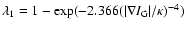
Smoothing is reduced in the direction of the image gradient if the gradient magnitude exceeds the threshold value
.
Smoothing is reduced in the direction of the image gradient if the gradient magnitude exceeds the threshold value  .
Thus anisotropic diffusion has the advantage of smoothing small noise fluctuations in the image whilst preserving large gradients.
The images are filtered over a scale equivalent to 1.4 pixel, with a value of
.
Thus anisotropic diffusion has the advantage of smoothing small noise fluctuations in the image whilst preserving large gradients.
The images are filtered over a scale equivalent to 1.4 pixel, with a value of
 DN pixel-1 and
are denoted as
DN pixel-1 and
are denoted as  .
.
Table 1:
Wave parameters of propagating wave packets.
Four tadpole-ray edges are selected (see Fig. 1b) and
their transverse displacement, ,
is determined in a y-t slice of
as a function of t at each fixed height x.
In such a slice, the location of an edge is initially selected interactively by
eye.
A more sophisticated, automated method, which builds an edge by connecting
regions in binary maps of thresholded gradients in y, has also been attempted.
This gives similar, but noisier results than the interactive method.
Especially where the choice of edge is not obvious, an interactive method gives better confidence.
The exact location of the edge is found by fitting locally for each t a Gaussian to
 .
The width of the Gaussian is taken as the error
.
The width of the Gaussian is taken as the error
 on
on
 .
By repeating this procedure for each height x, a map of the edge displacement,
,
is constructed.
.
By repeating this procedure for each height x, a map of the edge displacement,
,
is constructed.
Figure 2 shows
for each of the four edges as a function of time t and distance x.
All four edges show a pattern similar to Fig. 1c.
Firstly, for x > 30-40 Mm one or several wave packets, corresponding to the tadpole tail oscillations, are seen propagating sunwards at speeds above 100 km s-1.
Secondly, at lower heights (x < 40 Mm) and at later times a
repetitive pattern can be seen propagating sunwards at lower speeds of approximately 10 km s-1.
Innes et al. (2003b) concluded
that the slower propagating repetitive pattern
seen in
data slices similar to Fig. 1c
are due to shrinking loops with different temperatures having emission
in and out of the 195 Å bandpass.
Figure 2 suggests that these loops exhibit some transverse motions.
These motions, though, are small and slow,
and difficult to see in y-t data slices.
We are therefore not confident of the identification of these slower motions as wave phenomena,
and concentrate on the faster motions.
The signatures of the propagating wave packets are measured as follows.
A background, a boxcar running average of width 300 s by 5.5 Mm, is subtracted from
to
give
 .
Initially the passage time at each height of a selected wave extremum is deduced by fitting a polynomial t0(x) on visually selected points in
.
Initially the passage time at each height of a selected wave extremum is deduced by fitting a polynomial t0(x) on visually selected points in
 .
This curve is used to construct a time lag matrix,
.
This curve is used to construct a time lag matrix,
 ,
where the value of each element is the time lag nearest to
t0(xi) - t0(xj) for which
the correlation function
,
where the value of each element is the time lag nearest to
t0(xi) - t0(xj) for which
the correlation function
 is maximal.
This calculation is repeated twenty times, each time substituting
by
is maximal.
This calculation is repeated twenty times, each time substituting
by
 where r is a random number taken from a normal distribution of unity width.
The average and standard deviation are taken as the final value and error estimate of
.
The sunward directed phase speed,
where r is a random number taken from a normal distribution of unity width.
The average and standard deviation are taken as the final value and error estimate of
.
The sunward directed phase speed,
 ,
is constructed as
the inverse of the derivative of the time lag matrix in the j-direction averaged over j with a Gaussian weighing function of width 200s and localised at j=i.
A straight line is fitted to
,
is constructed as
the inverse of the derivative of the time lag matrix in the j-direction averaged over j with a Gaussian weighing function of width 200s and localised at j=i.
A straight line is fitted to
 to give the curve
![$V_{\rm ph}(x) = V_{\rm ph0} [1 - (x - x_0)/L_V]^{-1}$](/articles/aa/full/2005/06/aagi302/img25.gif) where
where
 is the sunward phase speed in km s-1 at height
x0 = 45.6 Mm
and LV is expressed in Mm.
The deceleration, a, is calculated, using the fitted curve for
,
from
is the sunward phase speed in km s-1 at height
x0 = 45.6 Mm
and LV is expressed in Mm.
The deceleration, a, is calculated, using the fitted curve for
,
from
 as
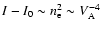
a(x) = a0 [1 - (x - x0)/LV]-3 where
as
a(x) = a0 [1 - (x - x0)/LV]-3 where
 .
.
![\begin{figure}
\par\includegraphics[width=5cm,clip]{2183fig3a.eps}\hspace*{2mm}
...
...s}\hspace*{2mm}
\includegraphics[width=5cm,clip]{2183fig3f.eps}
\end{figure}](/articles/aa/full/2005/06/aagi302/Timg28.gif) |
Figure 3:
a)-b) Phase speed and displacement amplitude as a function of distance x for
wave packets 1 and 3.
In the plot of the phase speed, the thick, solid line is an inverse linear fit
and the dashed line is the phase speed derived from t0(x).
In the plot of the amplitude, the solid line is a fitted exponential curve and the
dashed line represents the minimum amplitude that can be resolved, i.e. half a TRACE pixel size. c) Wave packet phase speeds
and periods P from
Table 1 as a function of time. The measurements from edges C and D are highlighted with solid circles. The dashed line is a linear fit through those points. |
| Open with DEXTER |
The period and amplitude of each wave packet is measured by fitting a function of the form
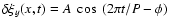 as a function of t for each height x
(see Fig. 4 for an illustration).
The period remains constant with height but the amplitudedecreases as the wave travels sunwards.
The amplitude is fitted by a function
as a function of t for each height x
(see Fig. 4 for an illustration).
The period remains constant with height but the amplitudedecreases as the wave travels sunwards.
The amplitude is fitted by a function
![$A(x) = A_0 ~ \exp[(x - x_0)/L_A]$](/articles/aa/full/2005/06/aagi302/img30.gif) ,
where A0 is the displacement amplitude at height x0 and LA is expressed in Mm.
From the measured phase speed and period, the wavelength is derived as
,
where A0 is the displacement amplitude at height x0 and LA is expressed in Mm.
From the measured phase speed and period, the wavelength is derived as
 .
It has the same functional form as
except that
the quantity
is replaced by
.
It has the same functional form as
except that
the quantity
is replaced by
 .
.
The measurements of the propagating wave packets are shown in Table 1.
Measurements of wave packet 7 using Fig. 1c have been added.
The quantities  and
and  are the analysed time and space intervals.
Each wave packet in Table 1 has the following behaviour.
The period is constant and lies in the range of 90-260 s.
The phase speed and amplitude decrease with sunward propagation.
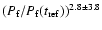
Figures 3a and b illustrate this for wave packets 1 (edge A) and 3 (edge B).
For x equal to 65 and 35 Mm the phase speeds are
in the ranges 200-700 km s-1 and 90-200 km s-1 respectively.
The wave velocity amplitude,
are the analysed time and space intervals.
Each wave packet in Table 1 has the following behaviour.
The period is constant and lies in the range of 90-260 s.
The phase speed and amplitude decrease with sunward propagation.
Figures 3a and b illustrate this for wave packets 1 (edge A) and 3 (edge B).
For x equal to 65 and 35 Mm the phase speeds are
in the ranges 200-700 km s-1 and 90-200 km s-1 respectively.
The wave velocity amplitude,
 ,
is in the range 8-40 km s-1.
The obtained phase speeds, periods and wavelengths are similar to those found by Seaton et al. (2003) and Cooper (2004) who measured the tadpole centre position at each time,
but for a limited range in x,
for two tadpoles corresponding to wave packets 3 and 5.
,
is in the range 8-40 km s-1.
The obtained phase speeds, periods and wavelengths are similar to those found by Seaton et al. (2003) and Cooper (2004) who measured the tadpole centre position at each time,
but for a limited range in x,
for two tadpoles corresponding to wave packets 3 and 5.
Figure 3c shows that the phase speeds and periods associated with wave packets in edges C and D are well correlated with time. A linear fit of these measurements gives
 [
[
 /1880] and
 /1633] where
 corresponds to 01:49:57 UT.
We propose that the transverse waves, seen in phase at the boundaries of tadpole tails and their neighbouring rays, are fast magnetoacoustic kink wave trains guided by the vertical ray-tadpole structure.
An MHD model with slab geometry may be used to characterise the structure (Roberts 1991).
A slab model is preferred over a cylindrical model because little is known about its extent along the line of sight, except that it cannot be narrow because then it would not be visible, as other coronal material within the line of sight would mask it.
Because the density is lower in the tadpole than in the ray, the waves may be surface modes.
Fast surface waves have a phase speed below the Alfvén speed in the denser ray (Rae & Roberts 1983).
If we take the the Alfvén speed,  ,
to lie in the plausible range of
500-1000 km s-1(increasing with height), then the observed phase speed magnitude is at least several hundreds
of km s-1 lower than the Alfvén speed.
This difference may be explained by considering the geometric configuration of the angles between wave propagation, tadpole and ray magnetic field directions and/or by the presence of upflows, possibly connected with the strong blue shifts observed with SUMER.
In the last case, the waves may be generated by negative energy mechanisms
(see e.g. Ruderman et al. 1996; Joarder 2002)
,
to lie in the plausible range of
500-1000 km s-1(increasing with height), then the observed phase speed magnitude is at least several hundreds
of km s-1 lower than the Alfvén speed.
This difference may be explained by considering the geometric configuration of the angles between wave propagation, tadpole and ray magnetic field directions and/or by the presence of upflows, possibly connected with the strong blue shifts observed with SUMER.
In the last case, the waves may be generated by negative energy mechanisms
(see e.g. Ruderman et al. 1996; Joarder 2002)
Edges C and D are seen to oscillate in phase for times after the data gap (see Fig. 1b),
which shows that the wave packet generated by one passing tadpole (corresponding to wave packet 6) penetrates beyond the neighbouring ray boundary.
The nature of the observed amplitude decrease is not obvious.
Besides dissipation, vertical structuring of the supra-arcade may be responsible.
The evolution of the phase speeds and periods of consecutive tadpole wave packets associated with the same ray (edges C and D) may be explained in terms of a density increase of the ray.
If for simplicity we assume that the ray intensity
 and
and
 ,
then
,
then
 and
and
 .
To test these relations we fit, using functions
.
To test these relations we fit, using functions
 and
and  ,
a power law to Iwith I0, a constant background intensity, and the power index as free parameters.
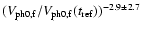
Best fits, averaged over x, correspond to power law indices of
,
a power law to Iwith I0, a constant background intensity, and the power index as free parameters.
Best fits, averaged over x, correspond to power law indices of
 and
and
 respectively
(see Fig. 5 for an illustration at x=x0).
The difference with the theoretical power law indices lies within the error.
The fits are only valid for times before 01:56 UT. The discrepancy at later times may be due to the use of a constant I0, or the evolution of the observation conditions.
respectively
(see Fig. 5 for an illustration at x=x0).
The difference with the theoretical power law indices lies within the error.
The fits are only valid for times before 01:56 UT. The discrepancy at later times may be due to the use of a constant I0, or the evolution of the observation conditions.
![\begin{figure}
\par\includegraphics[width=5.2cm,clip]{2183fig4.eps}
\end{figure}](/articles/aa/full/2005/06/aagi302/Timg49.gif) |
Figure 4:
Relative displacement
of wave packet 3 as a function of time for
x = 45.2 Mm.
The thick line is a fitted cosine function. |
| Open with DEXTER |
![\begin{figure}
\par\includegraphics[width=5.2cm,clip]{2183fig5.eps}
\end{figure}](/articles/aa/full/2005/06/aagi302/Timg50.gif) |
Figure 5:
Relative intensity
(I-I0)/I0 as a function of time of the ray between
edges C and D at x0=45.6 Mm.
The dashed and dot-dashed lines are best fit functions
 and
and
 respectively.
 |
| Open with DEXTER |
Innes & Wang (2003) presented SUMER Doppler shift measurements
for one of the tadpoles in this event (not studied here due to a TRACE data gap),
which showed oscillating red and blue shifts of about 10 km s-1.
This velocity amplitude is
of the same order as the velocity amplitudes reported here,
which indicates that the plane of wave polarisation is orientated at an angle between the
plane of the sky and the line-of-sight.
Acknowledgements
E.V. is grateful to PPARC for the financial support and to C. Foullon for useful comments.
V.M.N. acknowledges the support of a Royal Society Leverhulme Trust Senior Research Fellowship.
The authors are also grateful to the referee, D. Innes, and to E. DeLuca and D. Seaton.
- Asai, A., Yokoyama, T.,
Shimojo, M., & Shibata, K. 2004, ApJ, 605, L77 [NASA ADS] [CrossRef] (In the text)
- Aschwanden,
M. J., Fletcher, L., Schrijver, C. J., & Alexander, D. 1999,
ApJ, 520, 880 [CrossRef] (In the text)
- Dobrzycka,
D., Raymond, J. C., Biesecker, D. A., Li, J., & Ciaravella, A.
2002, ApJ, 588, 586 [NASA ADS] (In the text)
- Cooper, F. C. 2004,
Ph.D. Thesis, University of Warwick
(In the text)
- Gallagher, P.
T., Dennis, B. R., Krucker, S., Schwartz, R. A., & Tolbert, A.
K. 2002, Sol. Phys., 210, 341 [NASA ADS] [CrossRef] (In the text)
- Gallagher, P.
T., Lawrence, G. R., & Dennis, B. R. 2003, ApJ, 588, L53 [NASA ADS] [CrossRef] (In the text)
- Handy, B. N., Acton,
L. W., Kankelborg, C. C., et al. 1999, Sol. Phys., 187, 229 [NASA ADS] [CrossRef] (In the text)
- Innes, D. E.,
McKenzie, D. E., & Wang, T. 2003a, Sol. Phys., 217, 247 [NASA ADS] [CrossRef]
- Innes, D. E.,
McKenzie, D. E., & Wang, T. 2003b, Sol. Phys., 217, 267 [NASA ADS] [CrossRef] (In the text)
- Innes, D. E., &
Wang, T. 2003, ESA SP-547, 479
(In the text)
- Joarder, P. S.
2002, A&A, 384, 1086 [EDP Sciences] [NASA ADS] [CrossRef] (In the text)
- Kundu, M. R.,
Garaimov, V. I., White, S. M., & Krucker, S. 2004, ApJ, 600,
1052 [NASA ADS] [CrossRef] (In the text)
- McKenzie, D. E.
2000, Sol. Phys., 195, 381 [NASA ADS] [CrossRef] (In the text)
- McKenzie, D.
E., & Hudson, H. S. 1999, ApJ, 519, L93 [NASA ADS] [CrossRef] (In the text)
- Nakariakov,
V. M., Ofman, L., DeLuca, E. E., Roberts, B., & Davila, J. M.
1999, Science, 285, 862 [NASA ADS] [CrossRef] (In the text)
- Rae, I. C., &
Roberts, B. 1983, Sol. Phys., 84, 99 [NASA ADS] [CrossRef] (In the text)
- Roberts, B. 1991,
Advances in solar system magnetohydrodynamics, ed. E. R. Priest,
& A. W. Hood (Cambridge University Press)
(In the text)
- Ruderman, M.
S., Verwichte, E., Erdélyi, R., & Goossens, M. 1996, J.
Plasma Phys., 56, 285 (In the text)
- Seaton, D. B.,
Deluca, E. E., Cooper, F. C., & Nakariakov, V. M. 2003,
American Astronomical Society, SPD meeting #34, #16.18
(In the text)
- Sheeley, N. R.,
Jr., & Wang, Y.-M. 2002, ApJ, 579, 874 [NASA ADS] [CrossRef] (In the text)
- Svestka, Z.,
Fárnik, F., Hudson, H. S., & Hick, P. 1998, Sol. Phys.,
182, 179 [NASA ADS] [CrossRef] (In the text)
- Wang, Y.-M., Sheeley,
N. R., Jr., Howard, R. A., St., & Cyr, O. C. 1999, Geophys.
Res. Lett. 26, 1203
(In the text)
- Warren, H. P.,
Bookbinder, J. A., Forbes, T. G., et al. 1999, ApJ, 527, L121 [NASA ADS] [CrossRef] (In the text)
- Weickert, J.
1997, in Scale-Space Theory in Computer Vision, Lect. Notes Comput.
Sci., 1252, ed. B. ter Haar Romeny, L. Florack, J. Koenderink,
& M. Viergever (Berlin: Springer), 3
(In the text)
Copyright ESO 2005
![\begin{figure}
\par\includegraphics[width=5cm,clip]{2183fig3a.eps}\hspace*{2mm}
...
...s}\hspace*{2mm}
\includegraphics[width=5cm,clip]{2183fig3f.eps}
\end{figure}](/articles/aa/full/2005/06/aagi302/img28.gif)