 log [M/H] +1,
2000 K
log [M/H] +1,
2000 K
 50 000 K at several surface gravities
![[*]](/icons/foot_motif.gif)
A&A 428, 1001-1005 (2004)
DOI: 10.1051/0004-6361:20041673
Research Note
log [M/H] +1,
2000 K
50 000 K at several surface gravitiesA. Claret
Instituto de Astrofísica de Andalucía, CSIC, Apartado 3004, 18080 Granada, Spain
Received 16 July 2004 / Accepted 26 September 2004
Abstract
Continuing our studies on stellar atmospheres (Claret 2000, 2004),
we present in this paper the limb-darkening coefficients for the Sloan photometric
system. The calculations cover a wide range of values of log g,
 ,
metallicities
and microturbulent velocities. The atmosphere models used are ATLAS and PHOENIX.
In addition to the traditional applications of the limb-darkening coefficients,
the present ones will be useful since the Sloan filters are
now being used in the interpretation of light curves of extrasolar transiting planets,
for example. The present calculations may also be useful, as a complement, for the Kepler mission,
dedicated to the search for terrestrial planets.
,
metallicities
and microturbulent velocities. The atmosphere models used are ATLAS and PHOENIX.
In addition to the traditional applications of the limb-darkening coefficients,
the present ones will be useful since the Sloan filters are
now being used in the interpretation of light curves of extrasolar transiting planets,
for example. The present calculations may also be useful, as a complement, for the Kepler mission,
dedicated to the search for terrestrial planets.
Key words: stars: atmospheres - stars: binaries: eclipsing - stars: low mass, brown-dwarfs - stars: planetary systems
The calculations of the limb-darkening coefficients (LDC) that we have done previously cover the needs of several fields of Astrophysics. However, less usual photometric systems are now being used or are planned to be used. That is the case of the space mission Kepler. As a complement and as an exploratory work, the Sloan filters are being used to monitor candidates of extrasolar planetary transits (Torres 2004). In this case, the need of the LDC for Sloan filters is clear. The aim of this short paper is to present such calculations.
Despite the field of application of the limb-darkening coefficients, the adopted law and the numerical method used should provide a good description of the distribution of the specific intensities. Simple laws such as the linear one are not accurate (Kinglesmith & Sobieski 1970; Manduca et al. 1977; Claret & Giménez 1990; Van Hamme 1993). Quadratic or root-square approximations provide better fittings only for a narrow range of spectral types (Díaz-Cordovés 1990). In order to overcome these limitations, a new non-linear law was introduced (Claret 2000, Paper I). Among the advantages of this new law, we can quote: a) a single law is valid for the whole HR diagram; b) it is capable of reproducing very well the intensity distribution; c) the flux, computed using such a law, is conserved within an acceptable tolerance; d) it can be applied to different filters, log g, effective temperatures, metallicities and microturbulent velocities; e) it can be applied with success even in irradiated atmospheres (Claret 2004); f) it can be applied also in models with spherical symmetry (Claret & Hauschildt 2003). We adopted the new non-linear law and the Least-Square Method (LSM) throughout this paper.
The numerical procedure and methodology used here, as well as the terrestrial
transmission,
detector sensitivity and reflectivity of the aluminium coated mirror, were
described in
detail in Paper I. The only difference is the filter
transmissions for
the Sloan system, which were taken from Fukugita et al. (1996,
their Fig. 1).
![\begin{figure}
\par\includegraphics[height=22.7cm,width=17cm,clip]{1673fig1.eps}
\end{figure}](/articles/aa/full/2004/48/aa1673/img6.gif) |
Figure 1: The ratio between the actual flux (F) and that computed using Eq. (5) (F'). Sloan filters, ATLAS models, log g= 4.5, solar abundance, microturbulet velocity = 2 km s-1. |
| Open with DEXTER | |
 and
and
 K as well as for 5 values of the microturburlent
velocities (0, 1, 2, 4, 8 km s-1).
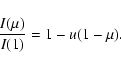
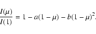
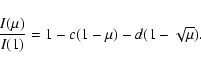
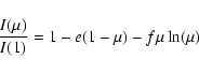
The LDC for the Sun and Vega are also available. We reproduce below
the adopted LDC laws in
order to facilitate the identification of the coefficients contained
in the tables:
K as well as for 5 values of the microturburlent
velocities (0, 1, 2, 4, 8 km s-1).
The LDC for the Sun and Vega are also available. We reproduce below
the adopted LDC laws in
order to facilitate the identification of the coefficients contained
in the tables:
Table 1: Limb-Darkening coefficients for u' g' r' i' z' bands (Least-Squares Method).
![\begin{figure}
\par\includegraphics[width=4.8cm,clip]{1673fig2.eps}
\end{figure}](/articles/aa/full/2004/48/aa1673/img9.gif) |
Figure 2: The linear coefficient u for ultraviolet bands. Continuous lines represent Strömgren u and asterisks denote Sloan u'. ATLAS models. log g= 4.5, solar abundance, microturbulet velocity = 2 km s-1. |
| Open with DEXTER | |
Linear
 |
(1) |
Quadratic
 |
(2) |
Square root
 |
(3) |
Logarithmic
 |
(4) |
 ,
,
 is the angle between the line of sight and the emergent
intensity. The new law introduced in Paper I is written as
is the angle between the line of sight and the emergent
intensity. The new law introduced in Paper I is written as
 |
(5) |
![\begin{figure}
\par\includegraphics[height=13.8cm,width=16.2cm,clip]{1673fig3.eps}
\end{figure}](/articles/aa/full/2004/48/aa1673/img17.gif) |
Figure 3: The linear coefficient u for u' g' r' i' z' following PHOENIX models (asterisks) and ATLAS (continuous line). log g= 4.5, solar abundance, microturbulet velocity = 2 km s-1. |
| Open with DEXTER | |
![\begin{figure}
\par\includegraphics[width=4.8cm,clip]{1673fig4.eps}
\end{figure}](/articles/aa/full/2004/48/aa1673/img18.gif) |
Figure 4:
The profiles of the specific intensities following a
non-linear law (Eq. (5)) for a model with
 K. PHOENIX models
(dashed line) and ATLAS (continuous line). log g = 4.5, solar
abundance, microturbulet velocity = 2 km s-1. K. PHOENIX models
(dashed line) and ATLAS (continuous line). log g = 4.5, solar
abundance, microturbulet velocity = 2 km s-1. |
| Open with DEXTER | |
Since these are the first calculations of LDC for the Sloan filters, it is convenient to compare the results with those derived for better known photometric systems. However, the only filter which can be really compared with a Sloan counter-part is the Strömgren u. Figure 2 shows such a comparison for ATLAS models. Note that the LDC derived for u' are systematically larger than those derived for the Strömgren u band, the maximum difference being around 10% at lower effective temperatures. The reason for these differences are in the effective wavelength of the two ultraviolet bands; the effective wavelength of the Sloan u' is slightly larger than its counterpart of Strömgren u. Of course, the general feature of the spectra near that spectral region and the sensitivity function also plays an important role.
Another interesting comparison that can be done is to investigate how the
ATLAS and PHOENIX models depend on the effective temperatures. Such a comparison
can only be done for the models that present similar input physics, such as log g,
metallicity, etc. In Fig. 3 are displayed the linear LDC for ATLAS (continuous
lines) and PHOENIX (asterisks) as a function of the effective temperature, for fixed values
of log g (4.5), metallicity (0.0) and microturbulent velocity (2 km s-1). The agreement
can be considered as acceptable but for lower effective temperatures (particularly at
log
around 3.5) and for u' band the comparison shows worse
agreement. Such differences can be attributed to the different input physics
in both codes of stellar atmospheres. In order to illustrate how both models
differ, we display in Fig. 4 the profiles of the specific intensities for a model
with
K, log g = 4.5, solar metallicity and 2 km s-1 of microturbulent
velocity at filter u'.
Table 1 summarizes the main
characteristics of the computed LDC. We encourage the reader to use the new non-linear
law since it provides a very good description of  )
(with merit functions about
103-104 times smaller than those for linear and bi-parametric approximations
(see Paper I). However, if one is interested in using the linear or bi-parametric
approximations, additional tables containing the respectives merit functions are also
available by request to evaluate the errors.
)
(with merit functions about
103-104 times smaller than those for linear and bi-parametric approximations
(see Paper I). However, if one is interested in using the linear or bi-parametric
approximations, additional tables containing the respectives merit functions are also
available by request to evaluate the errors.
Acknowledgements
R. Kurucz and P. H. Hauschildt are acknowledged for providing the data of their respective atmosphere models. G. Torres and V. Costa are also acknowledged for useful discussions. The Spanish MCYT (AYA2003-04651) is gratefully acknowledged for its support during the development of this work.