A&A 426, 707-715 (2004)
DOI: 10.1051/0004-6361:20047188
Collisional depolarization and transfer rates of spectral lines
by atomic hydrogen
IV. Application to ionised atoms
M. Derouich
1 -
S. Sahal-Bréchot
1
-
P. S. Barklem
2
1 - Observatoire de Paris-Meudon, LERMA UMR CNRS 8112, 5, Place Jules Janssen, 92195 Meudon Cedex, France
2 -
Department of Astronomy and Space Physics, Uppsala University, Box 515,
75120 Uppsala, Sweden
Received 9 February 2004 / Accepted 29 June 2004
Abstract
The semi-classical
theory of collisional depolarization of spectral lines
that we have applied to neutral atoms in previous papers
is extended to spectral lines
of singly ionised atoms. In order
to validate our general theory, we compare our results to
quantum chemistry calculations obtained for the particular cases of the 
 and
and

 states of the CaII ion. As a demonstration of the universality
of our theory and the easiness of its application, we calculate
depolarization and polarization
transfer rates for the
states of the CaII ion. As a demonstration of the universality
of our theory and the easiness of its application, we calculate
depolarization and polarization
transfer rates for the  state of the SrII
ion. Analytical
expressions of all rates as a function of local temperature are given.
Our results for the CaII ion are compared to recent quantum chemistry
calculations. A discussion of our results is presented.
state of the SrII
ion. Analytical
expressions of all rates as a function of local temperature are given.
Our results for the CaII ion are compared to recent quantum chemistry
calculations. A discussion of our results is presented.
Key words: Sun: atmosphere - atomic processes - line: formation - polarization
Observations of the linearly polarized radiation at the limb of the Sun
(known as the "second solar spectrum''), which is formed
by coherent scattering processes, show rich structures
(Stenflo & Keller 1997; Stenflo et al. 2000; Trujillo Bueno et al. 2001; Bommier & Molodij 2002). The linear polarization observations reported in the atlas recently published by Gandorfer (2000,2002) show significant polarization peaks in many spectral lines of
ions, e.g. NdII 5249 Å, EuII 4129 Å, CeII 4062 Å, CeII 4083 Å,
Ba II D2 4554 Å, ZrII 5350 Å, etc. Several surveys of the
scattering polarization throughout the solar spectrum
(Stenflo et al. 1980,1983a,b; see also the Q/I
observations of Stenflo et al. 2000 and the full Stokes-vector
observations of Dittmann et al. 2001) have shown that
ionised lines such as SrII 4078 Å and the IR triplet of CaII
are two of the more strongly polarized. The interpretation of these
observations requires the solution
of the coupling between the polarized radiative transfer equations (RTE)
and the statistical equilibrium equations (SEE) taking into account the
contributions of isotropic depolarizing collisions with neutral hydrogen. Depolarization and polarization transfer rates are currently available for ionised calcium levels, which have been obtained through sophisticated quantum chemistry methods which are accurate but cumbersome. Indeed, it is very difficult and sometimes not accurate to treat collision processes, involving heavy
ionised atoms like Ti II, Ce II, Fe II, Cr II, Ba II..., by standard quantum chemistry
methods.
It would be
useful to develop alternative methods capable of giving
results for many levels of ionised atoms rapidly and with reasonable accuracy.
and the IR triplet of CaII
are two of the more strongly polarized. The interpretation of these
observations requires the solution
of the coupling between the polarized radiative transfer equations (RTE)
and the statistical equilibrium equations (SEE) taking into account the
contributions of isotropic depolarizing collisions with neutral hydrogen. Depolarization and polarization transfer rates are currently available for ionised calcium levels, which have been obtained through sophisticated quantum chemistry methods which are accurate but cumbersome. Indeed, it is very difficult and sometimes not accurate to treat collision processes, involving heavy
ionised atoms like Ti II, Ce II, Fe II, Cr II, Ba II..., by standard quantum chemistry
methods.
It would be
useful to develop alternative methods capable of giving
results for many levels of ionised atoms rapidly and with reasonable accuracy.
The aim of this paper is
to extend the semi-classical theory of collisional depolarization of spectral
lines of neutral atoms by atomic hydrogen given in previous papers of this
series (Derouich et al. 2003a,b; Derouich et al. 2004;
hereafter Papers I, II and III respectively) to spectral lines of ions. This paper outlines the
necessary adjustments to the theory presented in Papers I, II and III for
extension to spectral lines of ions.
A great advantange of our theory is that it is not specific for a given perturbed ion, and may be easily applied to any singly ionised species. In order
to validate this theory, we have compared our results to quantum chemistry
calculations when possible. For this purpose, our results are presented and
compared with those obtained in the case of CaII levels by the quantum chemistry
method (Kerkeni et al. 2003). We also compare the results to the
depolarization rates computed with the Van der Waals potential.
Indeed, we have applied our method to calculate depolarization and polarization
transfer rates for the upper state 5 of the SrII 4078 Å
line.
of the SrII 4078 Å
line.
The main feature of the technique is the use of perturbation theory in calculating the interatomic potentials. A key parameter in this theory is  which approximates the energy denominator in the second-order interaction terms by an average value
(Paper I and ABO papers: Anstee 1992; Anstee & O'Mara 1991, 1995; Barklem 1998; Barklem & O'Mara 1997; Barklem et al. 1998).
A discussion of the effect of
variation on depolarization rates is presented. Finally, we show that the present semi-classical method
gives results in agreement with accurate but time consuming quantum chemistry calculations
to better than 15% for the CaII ion (T= 5000 K). Using our method it should now be possible to rapidly
obtain the data needed to interpret quantitatively the Stokes
parameters of the observed lines.
which approximates the energy denominator in the second-order interaction terms by an average value
(Paper I and ABO papers: Anstee 1992; Anstee & O'Mara 1991, 1995; Barklem 1998; Barklem & O'Mara 1997; Barklem et al. 1998).
A discussion of the effect of
variation on depolarization rates is presented. Finally, we show that the present semi-classical method
gives results in agreement with accurate but time consuming quantum chemistry calculations
to better than 15% for the CaII ion (T= 5000 K). Using our method it should now be possible to rapidly
obtain the data needed to interpret quantitatively the Stokes
parameters of the observed lines.
Under typical conditions of formation of observed lines in the solar atmosphere, the atomic system (atom, ion or molecule) suffers isotropic collisions with hydrogen atoms of the medium before it radiates. The states of the bath of hydrogen atoms are unperturbed.
In the tensorial formulation (Fano & Racah 1959; Messiah 1961; Fano 1963), the internal states of the perturbed
particles (here these particles are singly ionised atoms) are described by
the spherical tensor components
 of
the density matrix. Owing to the isotropy of the depolarizing collisions, the depolarization rates, polarization and population transfer rates are q-independent. The
term corresponding to the depolarizing collisions in the master equation is
given by
of
the density matrix. Owing to the isotropy of the depolarizing collisions, the depolarization rates, polarization and population transfer rates are q-independent. The
term corresponding to the depolarizing collisions in the master equation is
given by
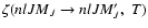
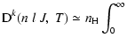
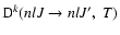
 is the collisional depolarization rate of the ionic level
(nlJ) at the local temperature T, where
is the collisional depolarization rate of the ionic level
(nlJ) at the local temperature T, where
 .
.
 is the destruction rate of population which is zero since elastic collisions (J=J') do not alter the population of the level (nlJ).
 is the destruction rate of orientation (related to circular polarization) and
 is the destruction rate of alignment of the level (nlJ) which is of interest in our astrophysics framework because it is related to the observed linear polarization.
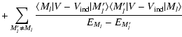
 is the fine structure transfer rate between the levels (nlJ)
  (nlJ') and
 is the polarization transfer rate between the levels
 ,
where
,
where
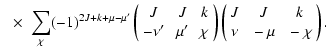
 ,
,
 if J<J' ( or if J > J' then
 ). In particular,
corresponds to collisional transfer of population (k=0), orientation (k=1) and alignment (k=2).
). In particular,
corresponds to collisional transfer of population (k=0), orientation (k=1) and alignment (k=2).
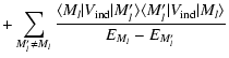
Higher order terms of
and
with
 can play a role in the SEE and have to be calculated. Note that, for the analysis of the linear polarization spectrum, only depolarization and polarization transfer rates with even k are need. Odd k-terms can be eliminated from the SEE.
and
can be written as a linear combination of the collisional transition rates between the fine stucture sublevels
 (Papers I, II and III, Sahal-Bréchot 1977); for depolarization rates
 and transfer rate of population
 ,
the coefficients of this linear combination are positive while the signs of the coefficients of the linear combination for transfer rates of rank
,
the coefficients of this linear combination are positive while the signs of the coefficients of the linear combination for transfer rates of rank  may be either positive or negative. This explains why transfer rates of rank
are significantly smaller
(Paper III). In our semi-classical theory, the collisional transition rate between the sublevels
may be either positive or negative. This explains why transfer rates of rank
are significantly smaller
(Paper III). In our semi-classical theory, the collisional transition rate between the sublevels
 is given by
(Papers I and II):
is given by
(Papers I and II):
 |
|
|
(2) |
where f(v) is the Maxwell distribution of
velocities for the local temperature T and  is the local hydrogen
atom number density.
I is the unit matrix and T = I-S is the so-called
transition matrix depending on the impact-parameter
is the local hydrogen
atom number density.
I is the unit matrix and T = I-S is the so-called
transition matrix depending on the impact-parameter  and relative
velocity
and relative
velocity  .
The collisional depolarization rates and the
collisional transfer rates, which are linear combinations of the
.
The collisional depolarization rates and the
collisional transfer rates, which are linear combinations of the
 given by Eq. (2), can
be expressed in terms of the T-matrix elements. The transition matrix T is functionally dependent on the interaction energy matrix of hydrogen in its ground state with the perturbed ion. Indeed, the transition
matrix elements in the dyadic basis are obtained by solving the time-dependent Schrödinger equation (Paper I)
given by Eq. (2), can
be expressed in terms of the T-matrix elements. The transition matrix T is functionally dependent on the interaction energy matrix of hydrogen in its ground state with the perturbed ion. Indeed, the transition
matrix elements in the dyadic basis are obtained by solving the time-dependent Schrödinger equation (Paper I)
 |
|
|
(3) |
 is the ion-hydrogen interaction used in this work and
 is the wave function of the system (ion+hydrogen).
 is the Hamiltonian of the system at the interatomic distance
  (Fig. 1).
![\begin{figure}
\par\includegraphics[width=8cm,clip]{0188fig1.eps}\end{figure}](/articles/aa/full/2004/41/aa0188-04/Timg62.gif) |
Figure 1:
The perturbed ion core (with charge Z=2) is located at A and the hydrogen perturbing
core (a proton) at P. Their valence electrons are denoted by 1 and 2
respectively. |
| Open with DEXTER |
The interaction potential for a singly ionised atom interacting with a
hydrogen atom
is treated in much the same way as for the neutral atom interaction with
hydrogen (Papers I, II and III; ABO papers). In the coordinate system of Fig. 1, V is given, in atomic units, by (Barklem & O'Mara 1998):
 |
(4) |
and atomic units are used hereafter.
 is
the part representing an inductive interaction between the excess charge
on the ionised atom and hydrogen atom. Quenching is neglected and thus we consider only the subspace nl (2l+1 states) and we denote the
product state of the two separated atoms at
by
is
the part representing an inductive interaction between the excess charge
on the ionised atom and hydrogen atom. Quenching is neglected and thus we consider only the subspace nl (2l+1 states) and we denote the
product state of the two separated atoms at
by
 .
By application of time-independent perturbation theory to the
second order, the interaction potential matrix elements are
given by:
.
By application of time-independent perturbation theory to the
second order, the interaction potential matrix elements are
given by:
EMl are the unperturbed energy eigenvalues of the isolated atoms. The expression for the second-order interaction can be greatly simplified
if we replace the energy denominator
EMl - EM'l, of each sum,
by a fixed average energy
and assume that for important separations
 .
This is
the Unsöld approximation (Unsöld 1927; Unsöld 1955).
.
This is
the Unsöld approximation (Unsöld 1927; Unsöld 1955).
 atomic units is the appropriate Unsöld energy value of the part of interaction,
 ,
between excess charge
on the ionized atom and hydrogen because this part is exactly the same as the H-H+ interaction. Indeed, Unsöld (1927) and Dalgarno & Lewis (Dalgarno & Lewis 1956, Eq. (16)) showed that
for the long-range H-H+ interaction. For the part of the interaction describing the interaction between the ion without the excess charge and hydrogen atom, the Unsöld value of -4/9 cannot be expected to be a good approximation (Barklem & O'Mara 1998). The reason that a value of -4/9 works well for neutrals is the fact that the separations of energy levels of the perturbed neutral atom are small compared to the separations between the ground level and the excited levels of the hydrogen atom, and thus the denominators are dominated by contributions from the H energy levels. For ions this is not the case. As a result
of the increased core charge, the energy level spacings are generally much
larger than for neutrals. It necessary therefore to determine
directly for each state of the ion. The appropriate value of
can be found via:
,
between excess charge
on the ionized atom and hydrogen because this part is exactly the same as the H-H+ interaction. Indeed, Unsöld (1927) and Dalgarno & Lewis (Dalgarno & Lewis 1956, Eq. (16)) showed that
for the long-range H-H+ interaction. For the part of the interaction describing the interaction between the ion without the excess charge and hydrogen atom, the Unsöld value of -4/9 cannot be expected to be a good approximation (Barklem & O'Mara 1998). The reason that a value of -4/9 works well for neutrals is the fact that the separations of energy levels of the perturbed neutral atom are small compared to the separations between the ground level and the excited levels of the hydrogen atom, and thus the denominators are dominated by contributions from the H energy levels. For ions this is not the case. As a result
of the increased core charge, the energy level spacings are generally much
larger than for neutrals. It necessary therefore to determine
directly for each state of the ion. The appropriate value of
can be found via:
 |
|
|
(6) |
where C6 is the Van der Waals constant averaged over all m substates. The C6 coefficient is given by the standard expression (see for example, Goodisman 1973):
 |
|
|
(7) |
 and
and
 are the dipole oscillator strengths
of all transitions to the state of interest l for the perturbed ion and the
ground state k for the neutral hydrogen atom.
are the dipole oscillator strengths
of all transitions to the state of interest l for the perturbed ion and the
ground state k for the neutral hydrogen atom.  and
and  are the
energy eigenvalues of the hydrogen and ionised atom respectively.
More details about the calculation of C6 are given in Barklem & O'Mara
(1998) and references therein.
The quantity
are the
energy eigenvalues of the hydrogen and ionised atom respectively.
More details about the calculation of C6 are given in Barklem & O'Mara
(1998) and references therein.
The quantity
 is the mean square distance between the valence
electron and the perturbed ion core located at A (Fig. 1),
is the mean square distance between the valence
electron and the perturbed ion core located at A (Fig. 1),
 |
|
|
(8) |
Pn*l are the the radial wavefunctions (note
 )
of the valence electron of the
perturbed atom (Anstee 1992; Seaton 1958). n* is the effective principal quantum number corresponding to the state
)
of the valence electron of the
perturbed atom (Anstee 1992; Seaton 1958). n* is the effective principal quantum number corresponding to the state
 of the
valence electron (Papers I, II and III).
of the
valence electron (Papers I, II and III).
Using the Unsöld approximation the expression for
becomes
of Eq. (9) is the so-called Rayleigh-Schrödinger-Unsöld
(RSU) potential. For computing
it is essential to determine
in
an independent calculation, as seen in Barklem & O'Mara (1998,2000).
Thus for ionized atoms it is not possible to tabulate cross-sections as for neutral
atoms (Papers I, II and III). Any calculations for depolarization and transfer of polarization involving ions must proceed line by line.
Considering a collision between a perturbed ion A and
hydrogen atom H (Fig. 1). Calculation of the depolarization and transfer rates follows essentially the steps listed below:
- 1.
- calculation of the required atomic wavefunctions of the system A+H;
- 2.
- determination of
directly for each state of the ion using Eq. (6);
- 3.
- numerical evaluation of the RSU interaction energy of the system A+H given by
Eq. (9);
- 4.
- use of these interaction potentials in the Schrödinger equation
describing the evolution of A+H collisional system in
order to
obtain the probabilities of depolarization and polarization transfer for a given impact parameter and a
relative velocity (more details in Paper I; see also Papers II and III);
- 5.
- calculation of depolarization and polarization transfer cross-sections for each relative velocity by integration over
impact parameters;
- 6.
- integration of cross-sections over the Maxwell distribution of velocities
to obtain the semi-classical depolarization and polarization transfer rates
for a range of local temperatures of the medium.
![\begin{figure}
\par\includegraphics[width=5.5cm,clip]{0188fig2.eps}\end{figure}](/articles/aa/full/2004/41/aa0188-04/Timg88.gif) |
Figure 2:
Partial Grotrian diagram of CaII showing the levels and the spectral wavelengths in Å
of interest in this study. Note that the level spacings in not to scale. |
| Open with DEXTER |
An important point to emphasise is that this semi-classical method for the calculation of depolarization and polarization transfer rates is not specific for a given perturbed atom or ion. This method can be applied for any perturbed ion,
but we must calculate the
value for each case (Sect. 3). Let us
consider the case of the Ca+-H system in view of its importance in
astrophysics and because
it is possible to compare with recent calculations employing the quantum chemistry approach (Kerkeni 2003). The case of the IR triplet lines of CaII has been investigated by Manso Sainz & Trujillo Bueno 2001,2003 and by Trujillo Bueno & Manso Sainz 2001, adopting
multilevel model of ionized calcium. The term levels associated to the IR triplet lines of
CaII (8498 Å, 8542 Å, and 8662 Å) are
 ,
,
 ,
,
 and
and
 (Fig. 2). The H and K lines occur at 3969 Å and 3933 Å respectively (Fig. 2); their upper states are also the upper states of the IR triplet. Table 1 lists, for the states of interest in this work,
,
C6 and the corresponding Ep calculated via Eq. (6) (see Barklem & O'Mara 1998).
(Fig. 2). The H and K lines occur at 3969 Å and 3933 Å respectively (Fig. 2); their upper states are also the upper states of the IR triplet. Table 1 lists, for the states of interest in this work,
,
C6 and the corresponding Ep calculated via Eq. (6) (see Barklem & O'Mara 1998).
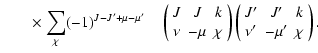
The depolarization transition probability is given by (Paper I; Sahal-Bréchot 1977):
Owing to the
selection rules for the 3j-coefficients, the summation over
 is reduced to a single term, since
 .
Integration over the impact-parameter b and the velocity
distribution for a temperature T of the medium can be
performed to obtain the depolarization rate which is given by:
.
Integration over the impact-parameter b and the velocity
distribution for a temperature T of the medium can be
performed to obtain the depolarization rate which is given by:
 v v 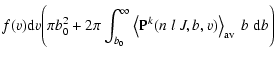 |
(11) |
where b0 is the cutoff impact-parameter and we use b0=3 a0 as
in Anstee & O'Mara (1991).
Table 1:
Average energy
for the interaction of CaII 3d and 4p
states with hydrogen in its ground state together with
and C6 values.
The excited state
 corresponds to total angular momentum J=1/2, the only non-zero depolarization rate is
 .
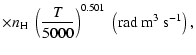
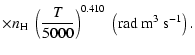
Figure 3 shows
as a function of the local temperature T.
.
Figure 3 shows
as a function of the local temperature T.
![\begin{figure}
\par\includegraphics[width=8.3cm,clip]{0188fig3.eps}\end{figure}](/articles/aa/full/2004/41/aa0188-04/Timg105.gif) |
Figure 3:
Destruction rate of orientation per unit H-atom density for the CaII ion,
 ,
as a function of temperature T.
/
is given in ,
as a function of temperature T.
/
is given in
 . . |
| Open with DEXTER |
The non-zero depolarization rates for the
state are
 ,
,
 and
and
 ,
and these rates are displayed in Fig. 4.
,
and these rates are displayed in Fig. 4.
![\begin{figure}
\par\includegraphics[width=8.3cm,clip]{0188fig4.eps}\end{figure}](/articles/aa/full/2004/41/aa0188-04/Timg111.gif) |
Figure 4:
Depolarization rates per unit H-atom density for the CaII ion,
 (k=1, 2, and 3), as a function of temperature T.
 /
are given in
. /
are given in
. |
| Open with DEXTER |
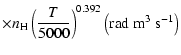
The non-zero depolarization rates associated to the
 and
and
 states are
 ,
,
 ,
,
 for
and
for
and
 ,
,
 ,
,
 ,
,
 and
and
 for
(see Figs. 5 and 6).
for
(see Figs. 5 and 6).
![\begin{figure}
\par\includegraphics[width=8.3cm,clip]{0188fig5.eps}\end{figure}](/articles/aa/full/2004/41/aa0188-04/Timg124.gif) |
Figure 5:
Depolarization rates per unit H-atom density for the CaII ion,
 (k=1, 2, and 3), as a function of temperature T.
 /
are given in
. /
are given in
. |
| Open with DEXTER |
![\begin{figure}
\par\includegraphics[width=7.9cm,clip]{0188fig6.eps}\end{figure}](/articles/aa/full/2004/41/aa0188-04/Timg127.gif) |
Figure 6:
Depolarization rates per unit H-atom density for the CaII ion,
 (k=1, 2, 3, 4, and 5), as a function of temperature T.
 /
are given in
. /
are given in
. |
| Open with DEXTER |
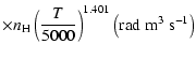
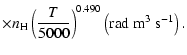
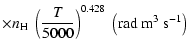
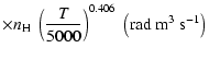
All of the rates for the
,
 ,
and
states of CaII are found to increase with temperature
in the range
,
and
states of CaII are found to increase with temperature
in the range
 K. As for neutral atoms, a functional form
 can usually be accurately fitted to these depolarization rates, where
  is the so-called velocity exponent
(Papers I, II and III). We find the following analytical expressions for the depolarization rates
for
is the so-called velocity exponent
(Papers I, II and III). We find the following analytical expressions for the depolarization rates
for
 K (except for
and
which are given for
K (except for
and
which are given for
 K):
K):
The collisional transfer transition probability is given by (Paper II; Sahal-Bréchot 1977):
As in Eq. (11), the polarization transfer rates
 follow from integration over the
impact parameters and the velocities with a Maxwellian distribution.
follow from integration over the
impact parameters and the velocities with a Maxwellian distribution.
Inelastic collisions with neutral hydrogen which leave the radiating atom in
a final state n'l' different from the initial one nl are neglected.
Only the polarization transfer rates inside the subspace nl are taken into account. Our transfer rates between the levels
,
(
 and
and
 )
are presented in Figs. 7 and 8 respectively.
)
are presented in Figs. 7 and 8 respectively.
 did not obey a power law of the form B
 .
However, we can provide the analytical expressions for the other non-zero transfer rates:
.
However, we can provide the analytical expressions for the other non-zero transfer rates:
![\begin{figure}
\par\includegraphics[width=7.9cm,clip]{0188fig7.eps}\end{figure}](/articles/aa/full/2004/41/aa0188-04/Timg193.gif) |
Figure 7:
Population and orientation transfer rates (k=0 and k=1), per unit H-atom density, as a function of temperature T. The rates are given in
. |
| Open with DEXTER |
![\begin{figure}
\par\includegraphics[width=7.9cm,clip]{0188fig8.eps}\end{figure}](/articles/aa/full/2004/41/aa0188-04/Timg195.gif) |
Figure 8:
Polarization transfer rates per unit H-atom density,
 ,
as a function of temperature T. The rates are given in
. ,
as a function of temperature T. The rates are given in
. |
| Open with DEXTER |
![\begin{figure}
\par\includegraphics[width=7.9cm,clip]{0188fig9.eps}\par\includeg...
...{0188fig10.eps}\par\includegraphics[width=7.9cm,clip]{0188fig11.eps}\end{figure}](/articles/aa/full/2004/41/aa0188-04/Timg196.gif) |
Figure 9:
Depolarization rates for k=2 as a function of temperature. Full lines: our results; dotted lines: quantum chemistry calculations (Kerkeni 2003); dot-dashed lines Van der Waals approximation. |
| Open with DEXTER |
It is important to notice that the depolarization rates
 as defined in this work (Eq. (11)) and the relaxation rates gk(J) as defined by Kerkeni et al. (2003) (Eq. (2), Sect. 3.2)
are not equivalent. Kerkeni et al. (2003) defines the depolarization cross-section (or relaxation rate gk(J)) as the sum of two terms: the term responsible exclusively for the depolarization of the level (nlJ) and the term corresponding to the fine structure transfer between the levels (nlJ)
(nlJ'). In our definition,
is only the depolarization of the level (nlJ), the fine structure transfer is not included. We calculate separately the rates
associated to fine structure transfer which are k-independent and proportional to the population transfer rates
as defined in this work (Eq. (11)) and the relaxation rates gk(J) as defined by Kerkeni et al. (2003) (Eq. (2), Sect. 3.2)
are not equivalent. Kerkeni et al. (2003) defines the depolarization cross-section (or relaxation rate gk(J)) as the sum of two terms: the term responsible exclusively for the depolarization of the level (nlJ) and the term corresponding to the fine structure transfer between the levels (nlJ)
(nlJ'). In our definition,
is only the depolarization of the level (nlJ), the fine structure transfer is not included. We calculate separately the rates
associated to fine structure transfer which are k-independent and proportional to the population transfer rates
 (Eq. (4) of Paper II).
For example, in
accordance with our definition
 but the
relaxation rates g0(J) from Kerkeni et al. (2003) are not necessarily zero. In
order to compare to the Kerkeni et al. (2003) results it is essential to
substract the part of gk(J) associated to fine structure transfer (
but the
relaxation rates g0(J) from Kerkeni et al. (2003) are not necessarily zero. In
order to compare to the Kerkeni et al. (2003) results it is essential to
substract the part of gk(J) associated to fine structure transfer (
 in Kerkeni et al. 2003). This it is nothing more than a difference in
definitions. Nevertheless, this difference should be taken into account when writing
the SEE.
We now compare our alignment depolarization rates with the quantum chemistry depolarization rates (Kerkeni et al. 2003) and the alignment depolarization rates obtained by replacing the RSU potential with improved Van der Waals potential,
in Kerkeni et al. 2003). This it is nothing more than a difference in
definitions. Nevertheless, this difference should be taken into account when writing
the SEE.
We now compare our alignment depolarization rates with the quantum chemistry depolarization rates (Kerkeni et al. 2003) and the alignment depolarization rates obtained by replacing the RSU potential with improved Van der Waals potential,
 ,
where C6 is taken from
Table 1. Note that the latter rates differ from the usual Van der Waals formula for the rates, because though we employ the van der Waals potential, the collision dynamics are treated using our theory, and the C6 value is accurately determined (whereas typically the approximation
,
where C6 is taken from
Table 1. Note that the latter rates differ from the usual Van der Waals formula for the rates, because though we employ the van der Waals potential, the collision dynamics are treated using our theory, and the C6 value is accurately determined (whereas typically the approximation
 is employed where
 is the polarisability of hydrogen).
In Fig. 9 we show our alignment depolarization rates with quantum chemistry depolarization rates (Kerkeni et al. 2003) and the improved Van der Waals rates. We display only the k=2 case which is related to the linear
depolarization (alignment). Reference to Fig. 9
shows that the Van der Waals potential significantly underestimates the depolarization
cross section. Our results show rather good agreement with quantum chemistry calculations.
In concrete terms, the percentage errors at T=5000 K with respect to quantum chemistry depolarization rates are 4.1% for
is the polarisability of hydrogen).
In Fig. 9 we show our alignment depolarization rates with quantum chemistry depolarization rates (Kerkeni et al. 2003) and the improved Van der Waals rates. We display only the k=2 case which is related to the linear
depolarization (alignment). Reference to Fig. 9
shows that the Van der Waals potential significantly underestimates the depolarization
cross section. Our results show rather good agreement with quantum chemistry calculations.
In concrete terms, the percentage errors at T=5000 K with respect to quantum chemistry depolarization rates are 4.1% for
 ;
4.6% for
;
4.6% for
 and 7.3% for
 .
The errors for the other depolarization and transfer rates are similar to the errors for the destruction rates of alignment (in general, less than 15%). This similarity is expected since all
rates orginate from the same collisional processes.
.
The errors for the other depolarization and transfer rates are similar to the errors for the destruction rates of alignment (in general, less than 15%). This similarity is expected since all
rates orginate from the same collisional processes.
![\begin{figure}
\par\includegraphics[width=7.9cm,clip]{0188fig12.eps}\end{figure}](/articles/aa/full/2004/41/aa0188-04/Timg210.gif) |
Figure 10:
Depolarization cross section enhancement due to a Gaussian local
perturbation of the potential. Cross sections are calculated for
the relative velocities:
 , ,
 and
and
 . . |
| Open with DEXTER |
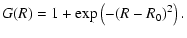
To assess the sensitivity of the calculations to the accuracy of the potentials at various separations we make calculations with potentials where we have introduced local perturbations.
The interaction potential (1s,
 )
is multiplied by a Gaussian magnification factor of the form (Anstee & O'Mara 1991):
)
is multiplied by a Gaussian magnification factor of the form (Anstee & O'Mara 1991):
 |
|
|
(18) |
R0 is the position where the variation of
reaches its
maximum value (the interaction potential  ,
,
 doubles). Figure 10 shows the depolarization cross-section
calculated with varying R0. It is clear
that the values of R0 inducing depolarization cross-section enhancement confirm the fundamental result found already for neutral atoms: the interactions of importance for the depolarization cross-section (or depolarization rate)
calculations are the intermediate-range interactions (Papers I, II and III). The principal differences between the RSU potentials and those from quantum chemistry occur at small interatomic separations. It is for this reason that we
obtain rather good agreement with quantum chemistry calculations. The Van der Waals interaction potentials are inaccurate at the intermediate region, and this explains why these potentials underestimate the depolarization cross
sections.
doubles). Figure 10 shows the depolarization cross-section
calculated with varying R0. It is clear
that the values of R0 inducing depolarization cross-section enhancement confirm the fundamental result found already for neutral atoms: the interactions of importance for the depolarization cross-section (or depolarization rate)
calculations are the intermediate-range interactions (Papers I, II and III). The principal differences between the RSU potentials and those from quantum chemistry occur at small interatomic separations. It is for this reason that we
obtain rather good agreement with quantum chemistry calculations. The Van der Waals interaction potentials are inaccurate at the intermediate region, and this explains why these potentials underestimate the depolarization cross
sections.
![\begin{figure}
\par\includegraphics[width=7.9cm,clip]{0188fig13.eps}\end{figure}](/articles/aa/full/2004/41/aa0188-04/Timg216.gif) |
Figure 11:
Dependence on
of the destruction rate of alignment
 5000 K)/.
 |
| Open with DEXTER |
The depolarization and transfer rates for the
and
states are calculated for
 and -1.236 respectively. As a check on the sensivity of our results to the precision of the calculations of ,
we have calculated the destruction rate of alignment
and -1.236 respectively. As a check on the sensivity of our results to the precision of the calculations of ,
we have calculated the destruction rate of alignment
 by varying
in Eq. (9). Note that when
decreases, the interaction potential decreases and so
also decreases (Fig. 11). The depolarization rate shows only an extremly weak variation with .
An
by varying
in Eq. (9). Note that when
decreases, the interaction potential decreases and so
also decreases (Fig. 11). The depolarization rate shows only an extremly weak variation with .
An
 variation of 25%, with respect to the value
,
corresponds to a change of less than 5% in the calculated depolarization rates. It should not concluded that this is a general property of the depolarization rates for all states of all ionised atoms. Reference to Fig. 11 shows a rather strong dependence of the depolarization rates on
for
variation of 25%, with respect to the value
,
corresponds to a change of less than 5% in the calculated depolarization rates. It should not concluded that this is a general property of the depolarization rates for all states of all ionised atoms. Reference to Fig. 11 shows a rather strong dependence of the depolarization rates on
for
 .
We expect, however, that the value of
is usually greater than 0.25 and the depolarization rates will not be greatly affected by possible error in the value of
(see Barklem & O'Mara 1998,2000).
.
We expect, however, that the value of
is usually greater than 0.25 and the depolarization rates will not be greatly affected by possible error in the value of
(see Barklem & O'Mara 1998,2000).
The Sr II 4078 Å
line was examined by Bianda et al. (1998), who wrote "...The rather large uncertainty in the depolarizing collision rate
introduces a corresponding uncertainty in the field-strength scale...''.
These authors have used the traditional Van der Waals approach to calculate collisional
rates. The 4078 Å
line is the resonance line of SrII: 
 .
We have computed the depolarization and polarization transfer rates of the levels
and
of SrII ion. The value of
.
We have computed the depolarization and polarization transfer rates of the levels
and
of SrII ion. The value of
 for the level
of SrII was adopted from Barklem & O'Mara (2000). We applied our method to obtaining the rates which are shown in Figs. 12
and 13. They were found to again obey a power law
for the level
of SrII was adopted from Barklem & O'Mara (2000). We applied our method to obtaining the rates which are shown in Figs. 12
and 13. They were found to again obey a power law
 and are given for
K by:
and are given for
K by:
![\begin{figure}
\par\includegraphics[width=7.9cm,clip]{0188fig14.eps}\end{figure}](/articles/aa/full/2004/41/aa0188-04/Timg238.gif) |
Figure 12:
Destruction rate of orientation per unit H-atom density for the SrII ion,
 ,
as a function of the temperature of the medium, T. ,
as a function of the temperature of the medium, T.
 /
is given in
. /
is given in
. |
| Open with DEXTER |
![\begin{figure}
\par\includegraphics[width=7.9cm,clip]{0188fig15.eps}\end{figure}](/articles/aa/full/2004/41/aa0188-04/Timg241.gif) |
Figure 13:
Depolarization rates,
 (k=1, 2, and 3), as a function of temperature T.
 /
are given in
. /
are given in
. |
| Open with DEXTER |
Between the term levels
and
there are only two non-zero polarization transfer rates which are given in Fig. 14. The analytical expressions for these rates for
K are:
![\begin{figure}
\par\includegraphics[width=7.9cm,clip]{0188fig16.eps}\end{figure}](/articles/aa/full/2004/41/aa0188-04/Timg248.gif) |
Figure 14:
Population and orientation transfer rates (k=0 and k=1) for the SrII ion, per unit H-atom density, as a function of temperature T. The rates are given in
. |
| Open with DEXTER |
We have adapted our semi-classical method of calculation of collisional depolarization of spectral lines of neutral atoms by atomic hydrogen to allow it to be used for singly ionised atoms. Comparison with recent quantum chemistry calculations for CaII at T=5000 K indicates an error less of than 8%. This is an encouraging result which supports the validity of our semi-classical approach. Using this method we should be able to calculate depolarization rates of the levels involved in
transitions of heavy
ionised atoms like SrII, Ti II, Ce II, Fe II, Cr II, BaII...
Calculations must proceed line by line because a suitable
value needs to be determined for each relevant state of the given ion. We have applied our
general method to calculate
depolarization and polarization transfer rates for the SrII state.
These calculations should allow a more accurate theoretical interpretation of the observed linear polarization of the SrII 4078 Å
line.
- Anstee, S. D., &
O'Mara, B. J. 1991, MNRAS, 253, 549 [NASA ADS] (In the text)
- Anstee, S. D. Ph.D.
Thesis, Univ. Queensland, 1992
(In the text)
- Anstee, S. D., &
O'Mara, B. J. 1995, MNRAS, 276, 859 [NASA ADS] (In the text)
- Barklem, P. S.,
& O'Mara, B. J. 1997, MNRAS, 290, 102 [NASA ADS] (In the text)
- Barklem, P. S.,
& O'Mara, B. J. 1998, MNRAS, 296, 1057 [NASA ADS] [CrossRef] (In the text)
- Barklem, P.
S., & O'Mara, B. J. 1998, MNRAS, 300, 863 [NASA ADS] [CrossRef] (In the text)
- Barklem, P.
S., & O'Mara, B. J. 2000, MNRAS, 311, 535 [NASA ADS] [CrossRef]
- Barklem, P. S. Ph.D.
Thesis , Univ. Queensland, 1998
(In the text)
- Barklem, P. S.,
Piskunov, N., & O'Mara, B. J. 2000, A&A, 142, 467 [NASA ADS]
- Bianda, M.,
Stenflo, J. O., & Solanki, S. K. 1998, A&A, 337, 565 [NASA ADS] (In the text)
- Bommier, V.,
& Molodij, G. 2002, A&A, 381, 241 [EDP Sciences] [NASA ADS] [CrossRef] (In the text)
- Dalgarno, A.,
& Williams, D. A. 1962, Proc. Phys. Soc. A (London), 69,
57 [NASA ADS] (In the text)
- Derouich,
M., Sahal-Bréchot, S., Barklem, P. S., & O'Mara, B. J.
2003a, A&A, 404, 763 [EDP Sciences] [NASA ADS] [CrossRef] (Paper I)
(In the text)
- Derouich,
M., Sahal-Bréchot, S., & Barklem, P. S. 2003b, A&A,
409, 369 [EDP Sciences] [NASA ADS] [CrossRef] (Paper II)
- Derouich, M.,
Sahal-Bréchot, S., & Barklem, P. S. 2004, A&A, 414,
369 [NASA ADS] (Paper III)
(In the text)
- Dittmann, O.,
Trujillo Bueno, J., Semel, M., & López Ariste, A. 2001, in
Advanced Solar Polarimetry: Theory, Observation, and
Instrumentation, ed. M. Sigwarth, ASP Conf. Ser., 236, 125
(In the text)
- Fano, U., & Racah, G.
1959, Irreducible Tensorial Sets (New York: Academic Press)
(In the text)
- Fano, U. 1963, Phys. Rev.,
131, 259 [NASA ADS] [CrossRef] (In the text)
- Gandorfer,
A. 2000, The Second Solar Spectrum: A high spectral resolution
polarimetric survey of scattering polarization at the solar limb in
graphical representation, vol. 1: 4625 Å
 to 6995 Å
(Hochschulverlag AG an der ETH Zurich)
(In the text)
to 6995 Å
(Hochschulverlag AG an der ETH Zurich)
(In the text) - Gandorfer,
A. 2002, The Second Solar Spectrum: A high spectral resolution
polarimetric survey of scattering polarization at the solar limb in
graphical representation, vol. 2: 3910 Å
to 4630 Å
(Hochschulverlag AG an der ETH Zurich)
- Goodisman,
J. 1973, Diatomic Interaction Potential Theory (New York: Academic
Press)
(In the text)
- Kerkeni, B.
2003, A&A, 402, 5 [EDP Sciences] [NASA ADS] [CrossRef] (In the text)
- Manso Sainz, R.,
& Trujillo Bueno, J. 2001, in Advanced Solar Polarimetry:
Theory, Observation, and Instrumentation, ed. M. Sigwarth, ASP
Conf. Ser., 236, 213
(In the text)
- Manso Sainz, R.,
& Trujillo Bueno, J. 2003, Phys. Rev. Lett., 91, 11 [NASA ADS]
- Messiah, A. 1961,
Mécanique Quantique (Paris: Dunod)
(In the text)
- Sahal-Bréchot, S.
1977, ApJ, 213, 887 [NASA ADS] [CrossRef] (In the text)
- Seaton, M. J.
1958, MNRAS, 118, 504 [NASA ADS] (In the text)
- Stenflo, J. O.,
Baur, T. G., & Elmore, D. F. 1980, A&A, 84, 60 [NASA ADS] (In the text)
- Stenflo, J.
O., Twerenbold, D., & Harvey, J. W. 1983a, A&A, 52, 161 [NASA ADS],
NASA ADS
- Stenflo, J.
O., Twerenbold, D., Harvey, J. W., & Brault, J. W. 1983b,
A&AS, 54, 505 [NASA ADS]
- Stenflo, J. O.,
& Keller, C. U. 1997, A&A, 321, 927 [NASA ADS] (In the text)
- Stenflo, J. O.,
Keller, C. U., & Gandorfer, A. 2000, A&A, 355, 789 [NASA ADS] (In the text)
- Trujillo
Bueno, J., & Collados, M., Paltou, F., & Molodij, G. 2001,
in Advanced Solar Polarimetry, Proc. 20th NSO/Sac Peak Summer
Workshop, ed. M. Sigwarth, ASP Conf. Ser., 236, 141
(In the text)
- Trujillo
Bueno, J., & Manso Sainz, R. 2001, in Magnetic Fields Across
the Hertzsprung-Russell Diagram, ed. G. Mathys, S. K. Solanki,
& D. T. Wickramasinghe (San Francisco: ASP), ASP Conf. Ser.,
248, 83
(In the text)
- Unsöld, A. L.
1927, Zeitschrit für Physik, 43, 574 [NASA ADS] (In the text)
- Unsöld, A. L.
1955, Physik der Stern Atmosphären (Zweite Auflage)
(In the text)
Copyright ESO 2004

![\begin{figure}
\par\includegraphics[width=8cm,clip]{0188fig1.eps}\end{figure}](/articles/aa/full/2004/41/aa0188-04/img62.gif)
![\begin{figure}
\par\includegraphics[width=5.5cm,clip]{0188fig2.eps}\end{figure}](/articles/aa/full/2004/41/aa0188-04/img88.gif)
![\begin{figure}
\par\includegraphics[width=8.3cm,clip]{0188fig3.eps}\end{figure}](/articles/aa/full/2004/41/aa0188-04/img105.gif)
![\begin{figure}
\par\includegraphics[width=8.3cm,clip]{0188fig4.eps}\end{figure}](/articles/aa/full/2004/41/aa0188-04/img111.gif)
![\begin{figure}
\par\includegraphics[width=8.3cm,clip]{0188fig5.eps}\end{figure}](/articles/aa/full/2004/41/aa0188-04/img124.gif)
![\begin{figure}
\par\includegraphics[width=7.9cm,clip]{0188fig6.eps}\end{figure}](/articles/aa/full/2004/41/aa0188-04/img127.gif)


![\begin{figure}
\par\includegraphics[width=7.9cm,clip]{0188fig7.eps}\end{figure}](/articles/aa/full/2004/41/aa0188-04/img193.gif)
![\begin{figure}
\par\includegraphics[width=7.9cm,clip]{0188fig8.eps}\end{figure}](/articles/aa/full/2004/41/aa0188-04/img195.gif)
![\begin{figure}
\par\includegraphics[width=7.9cm,clip]{0188fig9.eps}\par\includeg...
...{0188fig10.eps}\par\includegraphics[width=7.9cm,clip]{0188fig11.eps}\end{figure}](/articles/aa/full/2004/41/aa0188-04/img196.gif)
![\begin{figure}
\par\includegraphics[width=7.9cm,clip]{0188fig12.eps}\end{figure}](/articles/aa/full/2004/41/aa0188-04/img210.gif)
![\begin{figure}
\par\includegraphics[width=7.9cm,clip]{0188fig13.eps}\end{figure}](/articles/aa/full/2004/41/aa0188-04/img216.gif)
![\begin{figure}
\par\includegraphics[width=7.9cm,clip]{0188fig14.eps}\end{figure}](/articles/aa/full/2004/41/aa0188-04/img238.gif)
![\begin{figure}
\par\includegraphics[width=7.9cm,clip]{0188fig15.eps}\end{figure}](/articles/aa/full/2004/41/aa0188-04/img241.gif)

![\begin{figure}
\par\includegraphics[width=7.9cm,clip]{0188fig16.eps}\end{figure}](/articles/aa/full/2004/41/aa0188-04/img248.gif)