A&A 425, 725-728 (2004)
DOI: 10.1051/0004-6361:20040531
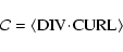
Vorticity and helicity of the solar supergranulation flow-field![[*]](/icons/foot_motif.gif)
P. Egorov - G. Rüdiger - U. Ziegler
Astrophysikalisches Institut Potsdam, An der Sternwarte 16, 14482 Potsdam, Germany
Received 26 March 2004 / Accepted 9 June 2004
Abstract
Box simulations of rotating convection are presented with the aim to
study the divergence-vorticity correlation  computed
from the horizontal velocity components of the turbulent flow field.
Our investigation is motivated by new observations of the solar velocity field
in the upper convection zone using the techniques of so-called time-distance
helioseismology
(Duvall et al. 1993). From such observations
can be
derived directly and because of the close relation to the helicity
it is an important quantity for solar dynamo theory.
The divergence-vorticity correlation obtained from the
simulations with Taylor number 103 is found to be in agreement with the
observations of supergranulation. In particular,
vanishes at the equator and is negative (positive) in the northern (southern) hemisphere.
For larger Taylor numbers the
amplitude of
increases, which is consistent with the increase
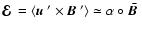
in strength of the Coriolis force acting on the turbulent flow.
We also demonstrate that the correlation
and the kinetic helicity
of the flow field have very similar spatial profiles. The observed values
of ,
therefore, yield a clear indication of the existence of
negative (positive) kinetic helicity in the surface layers of the
northern (southern) hemisphere.
computed
from the horizontal velocity components of the turbulent flow field.
Our investigation is motivated by new observations of the solar velocity field
in the upper convection zone using the techniques of so-called time-distance
helioseismology
(Duvall et al. 1993). From such observations
can be
derived directly and because of the close relation to the helicity
it is an important quantity for solar dynamo theory.
The divergence-vorticity correlation obtained from the
simulations with Taylor number 103 is found to be in agreement with the
observations of supergranulation. In particular,
vanishes at the equator and is negative (positive) in the northern (southern) hemisphere.
For larger Taylor numbers the
amplitude of
increases, which is consistent with the increase
in strength of the Coriolis force acting on the turbulent flow.
We also demonstrate that the correlation
and the kinetic helicity
of the flow field have very similar spatial profiles. The observed values
of ,
therefore, yield a clear indication of the existence of
negative (positive) kinetic helicity in the surface layers of the
northern (southern) hemisphere.
Key words: turbulence - Sun: granulation - Sun: helioseismology
There is no doubt that the magnetic activity of the cool stars is driven by the
turbulence in the outer convection zones which is subject to (density)
stratification and the global rotation. This finding is a common result of analytical considerations and numerical simulations. The existence of kinetic
helicity and current helicity which are both antisymmetric with respect
to the equator is central in those computations.
It is therefore natural to look for observational confirmations of this concept. A big step in this direction was the statistics of the current helicity
 |
(1) |
by Seehafer (1990) which has the same kind of equatorial (anti-) symmetry as the
dynamo- .
For
homogeneous global magnetic fields the latter
is related to the turbulent EMF
according to
.
For
homogeneous global magnetic fields the latter
is related to the turbulent EMF
according to
 .
The antiphase relation
.
The antiphase relation
 |
(2) |
by Keinigs (1983) between the -effect and the observed current helicity has suggested the
existence of an -effect which is positive (negative) in the northern (southern) hemisphere.
The kinetic helicity
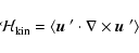 |
(3) |
which much earlier has been discussed as the physical background of
the -effect seemed to withstand direct observation.
Nevertheless, the rotational influence on the turbulence field should
be observable on the solar
surface. However, the effect is expected to be small and it is rather
complicated to prove as data only exist for the horizontal components u
and v of the flow.
In particular, the vertical component of the vorticity,
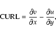 |
(4) |
and the (two-dimensional) divergence,
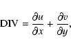 |
(5) |
of the horizontal velocity seem to be suitable quantities to study the
rotation-influenced surface flow field.
At the top of the convection zone a cellular network is formed by the
divergence of upflows and convergence of downflows. In the
compressible medium the
rising matter in the northern hemisphere expands and spins up under
the basic rotation in order to conserve its angular momentum.
In a righthand coordinate system with z pointing outwards these regions have
 and
rotate clockwise so that
and
rotate clockwise so that
 .
The downflows converge (
.
The downflows converge (
 ), compress and rotate in opposite
direction (
), compress and rotate in opposite
direction (
 )
under the influence of the Coriolis force. Therefore, lefthand spiral
motions dominate in the northern hemisphere. The divergence-vorticity
correlation
)
under the influence of the Coriolis force. Therefore, lefthand spiral
motions dominate in the northern hemisphere. The divergence-vorticity
correlation
 |
(6) |
is thus expected to be negative (positive) in the northern (southern) hemisphere. A
quasilinear calculation of this (nontrivial) correlation for anisotropic turbulence with the  -approximation leads to the result
 |
(7) |
(Rüdiger et al. 1999) which is of order 10-11 s-2 for correlation times of 1 day.
The candidates to study the rotational influence on the turbulence at the solar surface are mesogranules and
supergranules due to their nonmagnetic character.
The average cell sizes of supergranules are in the range 15-30 Mm
with predominantly
horizontal velocities. Recent observations (e.g., Hathaway et al. 2002) have shown
that the typical rms horizontal flow speed is  360 m/s while the rms
vertical flow speed is 30 m/s.
360 m/s while the rms
vertical flow speed is 30 m/s.
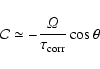
The rotational effect is estimated by the Coriolis number
 |
(8) |
where
 is
a typical correlation (life-) time and
is
a typical correlation (life-) time and
 is the angular velocity of the basic rotation.
The larger the scale of a velocity field the more sensitive is the flow to the
action of the Coriolis force.
For supergranulation one finds
is the angular velocity of the basic rotation.
The larger the scale of a velocity field the more sensitive is the flow to the
action of the Coriolis force.
For supergranulation one finds
 .
For mesogranulation
.
For mesogranulation  is of the order 10-2.
We did not find observations for the magnitude of
 ,
but only
maximum values of the divergence and vorticity were given (Brandt
et al. 1988;
Simon et al. 1988; Simon et al. 1994).
Wang et al. (1995) report indications of a negative divergence-vorticity
correlation
for the northern hemisphere.
,
but only
maximum values of the divergence and vorticity were given (Brandt
et al. 1988;
Simon et al. 1988; Simon et al. 1994).
Wang et al. (1995) report indications of a negative divergence-vorticity
correlation
for the northern hemisphere.
A clear detection of the influence of the Coriolis force is due to Duvall & Gizon (2000) and
Gizon & Duvall (2003) using the method of time-distance helioseismology (Duvall et al. 1993).
This technique provides both maps of the horizontal
divergence of the flows and information about two individual horizontal components
of the velocity. We shall use
their results for comparison with our numerical simulations.
The magnitude of the vorticity was found for the latitudinal interval of
 with zero at the equator and a value
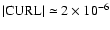 s-1
at the interval boundaries (see Fig. 7b in Gizon & Duvall 2003).
A vorticity of 10-6 s-1 corresponds to an angular velocity of
s-1
at the interval boundaries (see Fig. 7b in Gizon & Duvall 2003).
A vorticity of 10-6 s-1 corresponds to an angular velocity of
 or a typical circular velocity of
10 m/s. Gizon & Duvall (2003) detected a "significant correlation of a few percent between the vertical
vorticity and the horizontal divergence'' (their Fig. 7a).
Positive (negative) divergence in the northern hemisphere is correlated with
clockwise (counterclockwise) vorticity i.e.
or a typical circular velocity of
10 m/s. Gizon & Duvall (2003) detected a "significant correlation of a few percent between the vertical
vorticity and the horizontal divergence'' (their Fig. 7a).
Positive (negative) divergence in the northern hemisphere is correlated with
clockwise (counterclockwise) vorticity i.e.
 .
changes its sign in the southern hemisphere and
vanishes at the equator.
Both the sign and the latitudinal variation of
.
changes its sign in the southern hemisphere and
vanishes at the equator.
Both the sign and the latitudinal variation of
 characterize the effect of the Coriolis force on the flow.
The magnitude of the correlation
is obtained for the range of
latitudes
characterize the effect of the Coriolis force on the flow.
The magnitude of the correlation
is obtained for the range of
latitudes
![$[-45^{\circ}, 45^{\circ}]$](/articles/aa/full/2004/38/aa0531-04/img38.gif) where it varies from
where it varies from
 s-2to
s-2to
 s-2.
s-2.
Similar kinds of simulation, both the "local-box'' (e.g., Hathaway 1984;
Brummell et al. 1996, 1998)
and the full spherical shell (e.g., Miesch et al. 2000) have been used to study the effect of rotation
on laminar/turbulent, incompressible/compressible convection. A correlation of
counter-clockwise (cyclonic) flows with downdrafts and clockwise (anticyclonic) with updrafts
as well as a switch in the direction of circulations in the bottom part of convection zone
has been found for a wide range of Taylor number varying from 102 to 107.
The second result in its turn yields a sign reverse of the kinetic helicity along the radial direction; this has also been confirmed by simulations of Brummell et al. (1998) and Miesch et al. (2000).
In this paper the influence of the Coriolis force on the turbulence is simulated for the
solar surface flow pattern of supergranulation. We shall show that the results
of the simulations are close to both the quasilinear theory and the
observations. In the last section the relation between the DIV-CURL
correlation and the helicity is discussed with the result that the observations indicate a negative (positive) kinetic helicity in the northern (southern) hemisphere.
In this section we give a short description of the numerical model. The
3D numerical simulations of compressible, thermal convection under
the influence of rotation are performed in a small rectangular box
(Cartesian grid) which can be considered
as a small piece of a spherical shell. The domain is placed tangentially at different
colatitudes from
 (at the north pole) to
 (at the south pole) with a step of
 .
A sandwich configuration
which contains
a convectively unstable layer in between stably stratified
layers with overshooting convection has been constructed.
The height d of the convection zone is chosen as our length unit.
.
A sandwich configuration
which contains
a convectively unstable layer in between stably stratified
layers with overshooting convection has been constructed.
The height d of the convection zone is chosen as our length unit.
The box rotates around the polar axis from west to east.
The computational domain is
![$(x,y,z)\in[0,8d]\times[0,8d]\times[-2d,0]$](/articles/aa/full/2004/38/aa0531-04/img42.gif) discretized by
discretized by
 grid points which are uniformly distributed in
each coordinate direction.
grid points which are uniformly distributed in
each coordinate direction.
The governing equations describing thermal convection in a
stratified medium involving the effect of
the Coriolis force are
The notation for the physical variables is the following:  density,
P pressure, e thermal energy density, T temperature,
density,
P pressure, e thermal energy density, T temperature,
 velocity and
 the gravitational field.
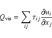
The remaining quantities in the equations are the viscous
stress tensor
given by
the gravitational field.
The remaining quantities in the equations are the viscous
stress tensor
given by
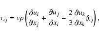 |
(12) |
where  denotes the kinematic viscosity coefficient, the
viscous heating term
denotes the kinematic viscosity coefficient, the
viscous heating term
 |
(13) |
and the thermal conductivity coefficient  .
.
The set (9)-(11) is closed through the
ideal gas equation of state
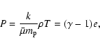 |
(14) |
where k is Boltzmann's constant,  is the atomic mass unit,
 is the mean molecular weight and
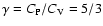 is the ratio of specific heats
  and
and  .
The chemical composition of the gas is ignored, hence
.
The chemical composition of the gas is ignored, hence
 .
.
The initial distribution of the physical quantities  corresponds to a
3-layer polytropic stratification.
All quantities are periodic in the horizontal
direction. At the bottom (z=-2) and the top (z=0) of the box
impermeable conditions are imposed for the vertical velocity while
the horizontal velocities satisfy a stress-free boundary condition.
The temperature and density are fixed at the top of the domain,
corresponds to a
3-layer polytropic stratification.
All quantities are periodic in the horizontal
direction. At the bottom (z=-2) and the top (z=0) of the box
impermeable conditions are imposed for the vertical velocity while
the horizontal velocities satisfy a stress-free boundary condition.
The temperature and density are fixed at the top of the domain,
 ,
and a constant heat flux is injected at the bottom.
,
and a constant heat flux is injected at the bottom.
The dimensionless parameters
 and
and  are used to control the simulations.
In our calculations
are used to control the simulations.
In our calculations
 and
and
 are fixed whereas
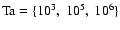 characterize the magnitude
of the angular velocity vector.
characterize the magnitude
of the angular velocity vector.
Equations (9)-(11) are solved with
the finite-difference, fractional-step code NIRVANA (Ziegler 1998,
1999).
Despite the simplifications in the numerical model (local box approximation,
gradients of temperature and density small compared to the real values in the solar convection zone)
the results discussed in the following are quite well in agreement with the observations.
The numerical simulations show an anisotropy between the vertical and horizontal
turbulent velocities. Vertical
motions dominate in the bulk of convection zone due to rising and descending flows.
At the top the flow becomes mostly horizontal due to divergent and convergent motions.
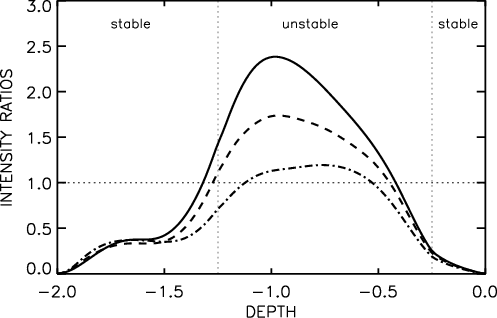
Figure 1 presents the computed anisotropy for
 and for different colatitudes in the northern hemisphere: in the upper part
of the convection zone the intensity of the horizontal velocities
and for different colatitudes in the northern hemisphere: in the upper part
of the convection zone the intensity of the horizontal velocities
 dominates over the vertical ones.
One can see there how the basic rotation modifies the intensity ratio with colatitude.
For slower rotation rates the dependence on colatitude clearly becomes weaker.
For the purpose of comparing our numerical results with the observations
we consider a region near the
top of the convection zone, for example at z=-0.3 (
dominates over the vertical ones.
One can see there how the basic rotation modifies the intensity ratio with colatitude.
For slower rotation rates the dependence on colatitude clearly becomes weaker.
For the purpose of comparing our numerical results with the observations
we consider a region near the
top of the convection zone, for example at z=-0.3 ( in depth) where
the horizontal cellular network is still visible as in the observations. The ratio
in depth) where
the horizontal cellular network is still visible as in the observations. The ratio
 at this point varies as
  30-45%
in all simulations.
30-45%
in all simulations.
 |
Figure 1:
The intensity ratio
in the box simulations for different colatitudes. The colatitudes are
(poles, solid),
(dashed) and
 (dot-dashed),
.
(dot-dashed),
. |
| Open with DEXTER |
To allow a direct comparison with the observed
a scaling factor
 is introduced where D is the depth of the convection
zone and
is introduced where D is the depth of the convection
zone and
 is
the sound speed at the top of the domain (z=0). Note that
is
the sound speed at the top of the domain (z=0). Note that  is the
same in all simulations. For solar
parameters i.e.
is the
same in all simulations. For solar
parameters i.e.
 and
and
 K,
we find
K,
we find
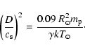 |
(15) |
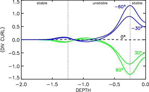
Figure 2 shows the computed correlation
 versus depth for
.
At the top of the convection
zone (z<-0.25)
is negative (positive) for the northern (southern) hemisphere.
As expected,
vanishes at the equator and its magnitude
increases toward the poles.
At the bottom of the convection zone and in the lower overshoot region
is relatively small and
it reverses its sign twice at
versus depth for
.
At the top of the convection
zone (z<-0.25)
is negative (positive) for the northern (southern) hemisphere.
As expected,
vanishes at the equator and its magnitude
increases toward the poles.
At the bottom of the convection zone and in the lower overshoot region
is relatively small and
it reverses its sign twice at
 and
and
 .
The results for
.
The results for
 qualitatively look similar except that
there is no sign reversal. The amplitude is reduced roughly by a factor of
2 compared with the
case.
qualitatively look similar except that
there is no sign reversal. The amplitude is reduced roughly by a factor of
2 compared with the
case.
 |
Figure 2:
The correlation
in the box simulations for various latitudes
after both horizontal and temporal averaging vs. depth for
. |
| Open with DEXTER |
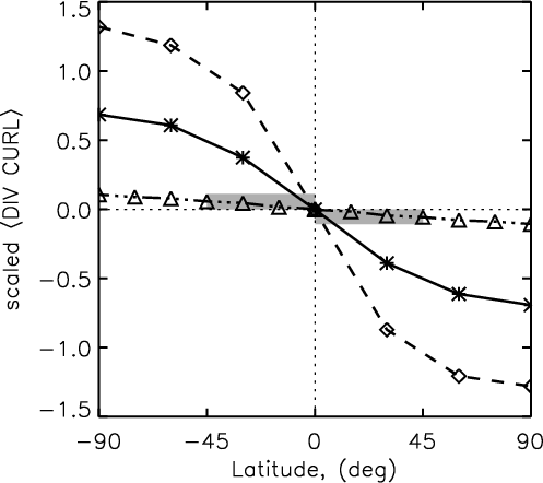
Figure 3 shows horizontal and time averages of
scaled by Eq. (15) vs. latitude plotted in comparison with observational results
indicated by the shaded area. In Fig. 3
triangles (
 ), asterisks (
)
and
diamonds (
)
denote the computed values of at a depth z=-0.3 (see Fig. 2) and for different latitudes
), asterisks (
)
and
diamonds (
)
denote the computed values of at a depth z=-0.3 (see Fig. 2) and for different latitudes
 .
.
 |
Figure 3:
Comparison of computed
with observational
data for
(triple-dot-dashed),
(solid) and
(dashed);
the numerical values are taken near the top of the convection zone (z=-0.3).
The shaded area covers the range of the observed data. |
| Open with DEXTER |
For slow rotation (
)
the correlation
is very
close to the observations. For higher Taylor numbers the amplitude of
 is
about one order of magnitude greater than the observed value for
supergranules. The
properties of the turbulence are shown in Table 1 for different rotation rates
and box inclinations. The rms value of
is
about one order of magnitude greater than the observed value for
supergranules. The
properties of the turbulence are shown in Table 1 for different rotation rates
and box inclinations. The rms value of  normalized by the sound
speed
is given as
characteristic for the flow field near the top of the convection zone.
With increasing rotation rate the rms velocities change from almost uniform
i.e. independent of
normalized by the sound
speed
is given as
characteristic for the flow field near the top of the convection zone.
With increasing rotation rate the rms velocities change from almost uniform
i.e. independent of  in the case
to a nonuniform distribution for
.
in the case
to a nonuniform distribution for
.
The coincidence between the simulations and
the observations illustrated in Fig. 3
is expected when comparing the Coriolis numbers in the simulations
with those prevailing in the supergranulation. The slower the box rotates
the smaller the influence of the Coriolis force
on the velocity field and, as a consequence,
would become smaller.
Although the Sun has
 ,
the supergranules rotate more
slowly than suggested by their Taylor number.
Indeed, for
we have a
similar to the value
estimated for the supergranulation flow field. This explains the good agreement
of the computed
with the observations. The obtained Coriolis numbers for the higher Taylor
number simulations are more related
to giant cells (also the typical cell size corresponds to giant cells),
hence, the effect
of rotation is at least one order of magnitude greater than the observed one.
Extrapolation of our results to the mesogranulation pattern leads to the
value of 10-11 s-2 for the maximum(poles)
correlation.
,
the supergranules rotate more
slowly than suggested by their Taylor number.
Indeed, for
we have a
similar to the value
estimated for the supergranulation flow field. This explains the good agreement
of the computed
with the observations. The obtained Coriolis numbers for the higher Taylor
number simulations are more related
to giant cells (also the typical cell size corresponds to giant cells),
hence, the effect
of rotation is at least one order of magnitude greater than the observed one.
Extrapolation of our results to the mesogranulation pattern leads to the
value of 10-11 s-2 for the maximum(poles)
correlation.
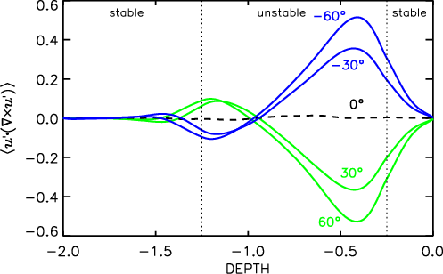
For the
case Fig. 4 shows the vertical
distribution of the kinetic helicity
(3) obtained by averaging over the horizontal directions and over
time. The comparison with
Fig. 2 reveals a close relationship of
and
 .
The signs of both quantities are clearly correlated.
Note that the vanishing of
at zero depth is forced
by the boundary condition at the outer edge of the upper overshooting region.
A relation
.
The signs of both quantities are clearly correlated.
Note that the vanishing of
at zero depth is forced
by the boundary condition at the outer edge of the upper overshooting region.
A relation
 has already been
formulated by Rüdiger et al. (1999), the presented arguments can
now be considered as numerically confirmed.Obviously, the observation of
the correlation
for supergranulation clearly indicates the
existence of negative (positive) kinetic helicity in the northern (southern)
hemisphere even close to the surface. The standard relation
between the -effect and kinetic helicity for hydrodynamic (!) turbulence is
has already been
formulated by Rüdiger et al. (1999), the presented arguments can
now be considered as numerically confirmed.Obviously, the observation of
the correlation
for supergranulation clearly indicates the
existence of negative (positive) kinetic helicity in the northern (southern)
hemisphere even close to the surface. The standard relation
between the -effect and kinetic helicity for hydrodynamic (!) turbulence is
 |
(16) |
(Krause & Rädler 1980).
According to Eq. (16) the observational results by
Gizon & Duvall (2003) would indicate the existence of a positive (negative)
-effect beneath the solar surface for the northern (southern) hemisphere.
 |
Figure 4:
Horizontally- and time-averaged kinetic helicity
vs. depth for
different latitudes in the box simulations for
.
Note the close relation of this quantity to the simulated correlation
given in
Fig. 2. The shape of the helicity curve is very close to results of
Miesch et al. (2000, their Fig. 22). |
| Open with DEXTER |
- Brandt, P. N.,
Scharmer, G. B., Ferguson, S., et al. 1988, Nature, 335, 238 [NASA ADS] [CrossRef] (In the text)
- Brummell, N.
H., Hurlburt, N. E., Toomre, J. 1996, ApJ, 473, 494 [NASA ADS] [CrossRef] (In the text)
- Brummell, N.
H., Hurlburt, N. E., Toomre, J. 1998, ApJ, 493, 955 [NASA ADS] [CrossRef] (In the text)
- Duvall, T. L.,
Jefferies, S. M., Harvey, J. W., & Pomerantz, M. A. 1993,
Nature, 362, 430 [NASA ADS] [CrossRef] (In the text)
- Duvall, T. L.,
& Gizon, L. 2000, Sol. Phys., 192, 177 [NASA ADS] [CrossRef] (In the text)
- Gizon, L., &
Duvall, T. L. 2003, Supergranulation Supports Waves, in Local and
Global Helioseismology: The Present and Future, ed. H.
Sawaya-Lacoste (Noordwijk: ESA Publications Division), 43
(In the text)
- Hathaway, D. H.
1982, Sol. Phys., 77, 341 [NASA ADS]
- Hathaway, D.
H., Beck, J. G., Han, S., & Raymond, J. 2002, Sol. Phys., 205,
25 [NASA ADS] [CrossRef] (In the text)
- Keinigs, R. K.
1983, Phys. Fluids, 76, 2558 [NASA ADS] [CrossRef] (In the text)
- Krause, F., &
Rädler, K.-H. 1980, Mean-field Magnetohydrodynamics and Dynamo
Theory (Oxford: Pergamon Press)
(In the text)
- Miesch, M. S.,
Elliott, J. R., Toomre, J., et al. 2000, ApJ, 532, 593 [NASA ADS] [CrossRef] (In the text)
- Rüdiger, G.,
Brandenburg, A., & Pipin, V. V. 1999, Astron. Nachr., 320,
135 [NASA ADS] [CrossRef] (In the text)
- Seehafer, N.
1990, Sol. Phys., 125, 219 [NASA ADS] (In the text)
- Simon, G. W., Title,
A. M., Topka, K. P., et al. 1988, ApJ, 327, 964 [NASA ADS] [CrossRef] (In the text)
- Simon, G. W., Brandt,
P. N., November, L. J., et al. 1994, in Solar Surface Magnetism,
ed. R. J. Rutten, & C.J. Schrijver (Dordrecht: Kluwer),
261
(In the text)
- Wang, Y., Noyes, R. W.,
Tarbell, T. D., & Title, A. M. 1995, ApJ, 447, 419 [NASA ADS] [CrossRef] (In the text)
- Ziegler, U. 1998,
Comput. Phys. Commun., 109, 111 [NASA ADS] (In the text)
- Ziegler, U. 1999,
Comput. Phys. Commun., 116, 65 [NASA ADS] (In the text)
Online Material
Table 1:
Properties of turbulence for different Taylor numbers and colatitudes
at z=-0.3.
Copyright ESO 2004