A&A 424, 545-559 (2004)
DOI: 10.1051/0004-6361:20041153
Discovery of optically faint obscured quasars with Virtual Observatory tools
P. Padovani
1 -
M. G. Allen2 -
P. Rosati3 -
N. A. Walton4
1 - ST-ECF, European Southern Observatory, Karl-Schwarzschild-Str. 2,
85748 Garching bei München, Germany
2 -
Centre de Données astronomiques de Strasbourg (UMR 7550), 11
rue de l'Université, 67000 Strasbourg, France
3 -
European Southern Observatory, Karl-Schwarzschild-Str. 2,
85748 Garching bei München, Germany
4 -
Institute of Astronomy, Madingley Road, Cambridge CB3 0HA, UK
Received 23 April 2004 / Accepted 2 June 2004
Abstract
We use Virtual Observatory (VO) tools to identify optically faint,
obscured (i.e., type 2) active galactic nuclei (AGN) in the two Great
Observatories Origins Deep Survey (GOODS) fields. By employing publicly
available X-ray and optical data and catalogues we discover 68 type 2 AGN
candidates. The X-ray powers of these sources are estimated by using a
previously known correlation between X-ray luminosity and X-ray-to-optical
flux ratio. Thirty-one of our candidates have high estimated powers
(
 erg/s) and therefore qualify as optically obscured quasars, the
so-called "QSO 2''. Based on the derived X-ray powers, our candidates are
likely to be at relatively high redshifts,
erg/s) and therefore qualify as optically obscured quasars, the
so-called "QSO 2''. Based on the derived X-ray powers, our candidates are
likely to be at relatively high redshifts,  ,
with the QSO 2 at
,
with the QSO 2 at
 .
By going
.
By going  3 mag fainter than previously known type 2 AGN in the two GOODS fields we are sampling a region of redshift - power space
which was previously unreachable with classical methods. Our method brings to 40 the number of QSO 2 in the GOODS fields, an improvement of a factor
3 mag fainter than previously known type 2 AGN in the two GOODS fields we are sampling a region of redshift - power space
which was previously unreachable with classical methods. Our method brings to 40 the number of QSO 2 in the GOODS fields, an improvement of a factor
 when compared to the only 9 such sources previously known. We derive
a QSO 2 surface density down to 10-15 erg cm-2 s-1 in the
0.5-8 keV band of
when compared to the only 9 such sources previously known. We derive
a QSO 2 surface density down to 10-15 erg cm-2 s-1 in the
0.5-8 keV band of  330 deg-2,
  of which is made up of previously known sources. This
is larger than current estimates and some predictions and suggests that the surface
density of QSO 2 at faint flux limits has been underestimated. This work
demonstrates that VO tools are mature enough to produce cutting-edge science
results by exploiting astronomical data beyond "classical'' identification
limits (
of which is made up of previously known sources. This
is larger than current estimates and some predictions and suggests that the surface
density of QSO 2 at faint flux limits has been underestimated. This work
demonstrates that VO tools are mature enough to produce cutting-edge science
results by exploiting astronomical data beyond "classical'' identification
limits ( )
with interoperable tools for statistical identification of
sources using multiwavelength information.
)
with interoperable tools for statistical identification of
sources using multiwavelength information.
Key words: astronomical data bases: miscellaneous -
methods: statistical - galaxies: quasars: general -
X-rays: galaxies
The unified model for active galactic nuclei (AGN) is largely accepted
(e.g., Urry & Padovani 1995; see also the very recent results by
Jaffe et al. 2004). The apparent disparate properties and
nomenclature of active galaxies can be explained by the physics of black
hole, accretion disk, jet, and obscuring torus convolved with the geometry
of the viewing angle. Type 1 sources are those in which we have an
unimpeded view
of the central regions and therefore exhibit the straight physics of AGN with
no absorption. Type 2 objects arise when the view is obscured by the
torus. While many examples of local, and therefore relatively low-power, type 2 AGN are known (the Seyfert 2s), it has been debated if their high-power
counterparts, that is optically obscured, radio-quiet type 2 QSO, exist.
Indeed, until
very recently, very few, if any, examples of this class were known. Apart from
their importance for AGN models, type 2 sources are expected to make a
significant fraction of the X-ray background (see, e.g., Comastri et al. 2001) and are therefore also cosmologically very
relevant. These sources are heavily reddened and therefore fall through the
"standard'' (optical) methods of quasar selection. The hard X-rays, however,
are thought to be able to penetrate the torus. Type 2 QSO, therefore, should
have narrow, if any, permitted lines (and might look like normal galaxies in
the optical/UV band), powerful hard X-ray emission, and, in some cases, a high
equivalent width Fe K line (e.g., Norman et al. 2002).
In this paper we use Virtual Observatory (VO) tools to identify 68 type 2 AGN candidates in the two Great Observatories Origins Deep Survey (GOODS) fields
(Giavalisco et al. 2004a), 1/2 of which qualify as QSO 2
candidates. Based on the properties of already known sources, we expect the
large majority of these to be obscured quasars whose identification is only
possible through their X-ray emission.
VO initiatives are now at a stage where prototype tools can be utilised to
produce scientific results. Real gains have been made in the areas of
accessing and describing remote data sets, manipulating image and catalogue
data, and performing remote calculations in a fashion similar to grid
computing. These prototype tools are enabled by the VO infrastructure and
interoperability standards that are being developed cooperatively by all the
VO projects under the auspices of the IVOA![[*]](/icons/foot_motif.gif) .
VO software is expected to mature significantly over the next 1-2 years as the
VO projects progress from demonstrations to building robust systems. In this
paper we have taken advantage of the first interoperability gains to produce
the "first science'' for the VO.
.
VO software is expected to mature significantly over the next 1-2 years as the
VO projects progress from demonstrations to building robust systems. In this
paper we have taken advantage of the first interoperability gains to produce
the "first science'' for the VO.
In Sect. 2 we present the data we have used, Sect. 3 discusses the tools
we employed, while Sect. 4 describes our method. Section 5 presents our
results, which are discussed in Sect. 6, while Sect. 7 summarizes our
conclusions. Throughout this paper spectral indices are written
 and we adopt a cosmological model with H0 = 70 km s-1 Mpc-1,
 ,
and
,
and
 .
.
We use for our purposes the two GOODS fields (Giavalisco et al.
2004a), namely the Hubble Deep Field-North (HDF-N) and the Chandra
Deep Field-South (CDF-S). Since GOODS includes some of the deepest
observations from space- and ground-based facilities, these are the most
data-rich, deep survey areas on the sky. The GOODS field centres (J2000.0) are
12 36
36 55
55 ,
+62
,
+62 14
14 15
15
 for the
HDF-N and 33230,
for the
HDF-N and 33230,
 4820
for
the CDF-S. Each field provides an area of approximately 10
4820
for
the CDF-S. Each field provides an area of approximately 10
 .
.
Deep X-ray (Chandra) catalogues are available for a larger region around both
fields (Alexander et al. 2003; Giacconi et al.
2002). For consistency, we use the catalogues produced by
Alexander et al. (2003) for both the 2 Ms HDF-N and 1 Ms CDF-S
data. These include 503 (HDF-N) and 326 (CDF-S) objects respectively, for a
total of 829 sources. The data cover the 0.5-8.0 keV band and the
catalogues provide counts and fluxes in various sub-bands. Note that, due to
the twice as long exposure time, the HDF-N reaches fainter X-ray
fluxes and includes a ( )
larger number of sources.
)
larger number of sources.
In the optical we use the publicly available GOODS Hubble Space Telescope (HST) Advanced Camera for Surveys (ACS) data (proposal ID 9583). The
observations consist of imaging in the F435W, F606W, F775W, and F850LP passbands, hereafter referred to as B, V, i, and z, respectively. We use
here version v1.0 of the reduced, calibrated, stacked, and mosaiced images and
catalogues as made available by the GOODS team.
Finally, identifications and redshifts through optical spectroscopy are
available from Barger et al. (2003) and Szokoly et al.
(2004) for the HDF-N and CDF-S respectively. We note that  of the X-ray sources in the GOODS fields have spectroscopic redshift
determinations. These sources are necessarily relatively bright, with
of the X-ray sources in the GOODS fields have spectroscopic redshift
determinations. These sources are necessarily relatively bright, with
 (HDF-N; only
  fainter than 24th mag) and
 (CDF-S; only
  fainter than 25th mag).
Astronomy is at a turning point. Major breakthroughs in telescope,
detector, and computer technology allow astronomical surveys to produce
massive amounts of images, spectra, and catalogues. These datasets cover the
sky at all wavelengths from  - and X-rays, optical, infrared,
through to radio. The VO is an international,
community-based initiative, to allow global electronic access to available
astronomical data, both space- and ground-based. The VO aims also to enable
data analysis techniques through a coordinating entity that will provide
common standards, wide-network bandwidth, and state-of-the-art analysis
tools.
- and X-rays, optical, infrared,
through to radio. The VO is an international,
community-based initiative, to allow global electronic access to available
astronomical data, both space- and ground-based. The VO aims also to enable
data analysis techniques through a coordinating entity that will provide
common standards, wide-network bandwidth, and state-of-the-art analysis
tools.
The Astrophysical Virtual Observatory Project (AVO) is conducting a research and demonstration programme
on the scientific requirements and technologies necessary to build a VO for
European astronomy. The AVO has been jointly funded by the European Commission
(under FP5 - Fifth Framework Programme) with six European organisations
participating in a three year Phase-A work programme.
The AVO project is driven by its strategy of regular scientific demonstrations
of VO technology. For this purpose an "AVO prototype'' has been built. The
prototype consists of a suite of interoperable software, plus a set of
conventions or standards for accessing remote data, and for launching remote
calculations. The main component of the software is based on the CDS Aladin
visualisation interface (Bonnarel et al. 2000). This prototype
VO portal (v. 1.003- )
allows efficient interactive manipulation of
image and catalogue data, and provides access to remote data archives and
image servers via the GLU registry of services.
)
allows efficient interactive manipulation of
image and catalogue data, and provides access to remote data archives and
image servers via the GLU registry of services.
The Aladin image server is an example of such a VO service. It describes the
images stored in the Aladin database using a data model (Images Distribuées
Hétérogènes pour l'Astronomie; IDHA), and provides image cutouts on
request. In this paper we make heavy use of cutouts of the GOODS data
available via this service. The prototype is also interoperable with the other
long standing CDS Vizier and SIMBAD services (Ochsenbein et al.
2000), and significant interoperability gains are achieved by
use of the VOTable format
for astronomical tables.
The prototype includes a catalogue cross matching service. This service allows
positional cross matching of two catalogues to find the best matched source,
all matching sources, or sources not matching within a given threshold radius
(in arcseconds). These three modes, plus the ability to compare directly with
the images from which the catalogues were generated, make for an extremely
efficient tool for which to perform cross matches and check for multiple, or
aberrant matches.
In addition to the AVO software, we have also made intensive use of the
Starlink topcat tool, and the VOIndia VOPlot plugin
to the prototype.
The two key physical properties that we use to identify type 2 AGN candidates are that they be obscured, and that they have sufficiently
high power to be classed as an AGN and not a starburst. To find these
candidates, we use a relatively simple method based on the X-ray and
optical fluxes.
Optical data alone are not sufficient for this purpose because at the
redshifts that we expect to find these sources the nuclear, AGN emission can
be diluted by the host galaxy. Indeed, Moran et al.
(2002) have shown that  of local Seyfert 2 galaxies
would be classified as normal galaxies if no decomposition of their optical
emission were available. However, AGN reveal themselves by their hard X-ray
emission and power. Ideally, to find type 2 AGN, one would need X-ray spectra
to select sources with flat spectral indices, indicative of absorption. The
typical count rates of the X-ray sources in the GOODS fields are however
relatively low for detailed spectral fitting and therefore we select sources
based on their X-ray hardness ratio, a measure of the fraction of hard photons
relative to soft photons.
of local Seyfert 2 galaxies
would be classified as normal galaxies if no decomposition of their optical
emission were available. However, AGN reveal themselves by their hard X-ray
emission and power. Ideally, to find type 2 AGN, one would need X-ray spectra
to select sources with flat spectral indices, indicative of absorption. The
typical count rates of the X-ray sources in the GOODS fields are however
relatively low for detailed spectral fitting and therefore we select sources
based on their X-ray hardness ratio, a measure of the fraction of hard photons
relative to soft photons.
To estimate the X-ray power for candidate type 2 sources we use the
correlation described by Fiore et al. (2003) between the
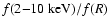 ratio and the hard X-ray power (see their Fig. 5). The basis
of this correlation is the fact that the
ratio is
roughly equivalent to the ratio between the nuclear X-ray power and the
host galaxy R band luminosity. Since the host galaxy R band luminosities
(unlike the X-ray power) show only a modest amount of scatter, this flux ratio
is a good indicator of X-ray power.
ratio and the hard X-ray power (see their Fig. 5). The basis
of this correlation is the fact that the
ratio is
roughly equivalent to the ratio between the nuclear X-ray power and the
host galaxy R band luminosity. Since the host galaxy R band luminosities
(unlike the X-ray power) show only a modest amount of scatter, this flux ratio
is a good indicator of X-ray power.
Each of the steps in our method, including our technique for
identifying the optical counterparts of the X-ray sources, are described
in detail below.
4.1 Selecting absorbed sources
The Alexander et al. (2003) catalogues provide counts in various
X-ray bands. We define the hardness ratio
 ,
where H is the
hard X-ray counts (2.0-8.0 keV) and S is the soft X-ray counts (0.5-2.0 keV). Following Szokoly et al. (2004) when H is an upper
limit we set
,
where H is the
hard X-ray counts (2.0-8.0 keV) and S is the soft X-ray counts (0.5-2.0 keV). Following Szokoly et al. (2004) when H is an upper
limit we set
 ,
while when S is an upper limit we set
,
while when S is an upper limit we set
 .
The
14 sources with upper limits in both H and S bands were excluded. Szokoly et al. (2004) have shown that absorbed, type 2 AGN are
characterized by
.
The
14 sources with upper limits in both H and S bands were excluded. Szokoly et al. (2004) have shown that absorbed, type 2 AGN are
characterized by
 .
We adopt this criterion and identify those
sources which have
as absorbed sources. We find 294 (CDF-S: 104,
HDF-N: 190) such absorbed sources which represent
.
We adopt this criterion and identify those
sources which have
as absorbed sources. We find 294 (CDF-S: 104,
HDF-N: 190) such absorbed sources which represent
 (
( Poisson errors are from Gehrels 1986) of the X-ray sources in the
Alexander catalogues. The hardness ratio distribution is shown in Fig. 1. We note that for an
Poisson errors are from Gehrels 1986) of the X-ray sources in the
Alexander catalogues. The hardness ratio distribution is shown in Fig. 1. We note that for an
 the flux in the 2-8 keV band used by Alexander et al. (2003) is only
  smaller than that in the commonly used 2-10 keV band. We also point out
that increasing redshift makes the sources softer (e.g., at z = 3 the
rest-frame 2-8 keV band shifts to 0.5-2 keV) so our selection
criterion will mistakenly discard some high-z type 2 sources, as pointed out
by Szokoly et al. (2004). The number of type 2 candidates we find
has therefore to be considered a lower limit.
smaller than that in the commonly used 2-10 keV band. We also point out
that increasing redshift makes the sources softer (e.g., at z = 3 the
rest-frame 2-8 keV band shifts to 0.5-2 keV) so our selection
criterion will mistakenly discard some high-z type 2 sources, as pointed out
by Szokoly et al. (2004). The number of type 2 candidates we find
has therefore to be considered a lower limit.
One commonly adopted definition of absorbed source is
 cm-2, where
  is the intrinsic absorption at the redshift of the source. We discuss below how this compares with our definition.
![\begin{figure}
\par\includegraphics[width=8.3cm,clip]{1153fig1.eps}
\end{figure}](/articles/aa/full/2004/35/aa1153/Timg46.gif) |
Figure 1:
The distribution of hardness ratios in the Alexander et al.
(2003) catalogues. We define as absorbed sources
to the right of the dashed line, that is having hardness ratio
. |
| Open with DEXTER |
The optical counterparts to the X-ray sources were selected by
cross-matching the absorbed X-ray sources with the GOODS ACS catalogues
(29 599 sources in the CDF-S, 32 048 in the HDF-N). The GOODS catalogues
contain sources that were detected in the z-band, with  photometry
in matched apertures (Giavalisco et al. 2004b). We checked for
possible offsets between the optical and X-ray astrometry by cross-matching
the full (CDF-S and HDF-N) Alexander catalogues with the GOODS catalogues
using a threshold radius of 1.25
(see below). In the HDF-N we
detected a systematic shift of -0.029
in RA, and -0.297
in
declination of the Alexander positions with respect to the GOODS positions,
and we applied this correction to the Alexander coordinates before doing
the cross-match.
photometry
in matched apertures (Giavalisco et al. 2004b). We checked for
possible offsets between the optical and X-ray astrometry by cross-matching
the full (CDF-S and HDF-N) Alexander catalogues with the GOODS catalogues
using a threshold radius of 1.25
(see below). In the HDF-N we
detected a systematic shift of -0.029
in RA, and -0.297
in
declination of the Alexander positions with respect to the GOODS positions,
and we applied this correction to the Alexander coordinates before doing
the cross-match.
Note that the ACS image areas for the CDF-S and the HDF-N are both smaller
than (and are completely within) their respective Chandra image fields. 546 out of the 829 sources in the Alexander catalogue (CDF-S: 222/326, HDF-N:
324/503) fall within the ACS image area. Of the 294 absorbed sources, 203 (CDF-S: 77, HDF-N: 126) fall within the ACS image area.
To find the optical counterparts of the absorbed X-ray sources, we initially
search for optical sources that lie within a relatively large threshold radius
of 3.5
(corresponding to the maximal  positional uncertainty
of the X-ray positions) around each X-ray source. This was done using the
cross match facility in the AVO prototype tool using the "best match'' mode.
positional uncertainty
of the X-ray positions) around each X-ray source. This was done using the
cross match facility in the AVO prototype tool using the "best match'' mode.
We find 195 "best'' matches, 76 in the CDF-S and 119 in the HDF-N. So, in the
CDF-S, all but one of the absorbed sources in the ACS image area have optical
counterparts. The remaining source, Alexander ID 213, falls within the 10
disk of a bright galaxy. In the HDF-N there are 7 absorbed sources within the image area that do not have an optical counterpart
(these 7 sources do however have optical matches in Barger et al.
(2003), although we note that most of these are below the 5 limit of their catalogue).
Since the 3.5
radius is large relative to the median positional error,
and given the optical source density the initial cross match inevitably
includes a number of false and multiple matches. To limit our sample to good
matches, we use the criterion that the cross match distance be less than the
combined optical and X-ray positional uncertainty for each
individual match. Applying this distance/error <1 criterion we limit the
number of matches to 168 (CDF-S: 65, HDF-N: 103). These matches are all within
a much smaller radius than our initial 3.5
threshold, with most of the
distance/error <1 matches being within 1.25
(and two matches at 1.4 and 1.5
).
Considering not only the best match but also the multiple matches
within a threshold radius of 1.25
(and distance/error <1)
we find 189 matches (CDF-S: 67, HDF-N: 122) to the 168 X-ray
sources. This means that our method of only considering the best
matches does discard 21 possibly valid matches in preference for a
closer match.
The number of false matches we expect to have, as detailed in Appendix A, is small, between 8 and 15%.
Our method requires R magnitudes in order to estimate the X-ray luminosity
via the Fiore et al. correlation. The ACS band closest to the R band is the
i band. We then convert the ACS i magnitudes to the R band assuming
 ,
which is the typical value we derive for previously known
type 2 AGN in the GOODS fields (see Sect. 6.1). The R band flux,
f(R), was then computed by converting R magnitudes to specific fluxes and
then multiplying by the width of the R filter (Zombeck 1990), as in Fiore et al. (2003).
,
which is the typical value we derive for previously known
type 2 AGN in the GOODS fields (see Sect. 6.1). The R band flux,
f(R), was then computed by converting R magnitudes to specific fluxes and
then multiplying by the width of the R filter (Zombeck 1990), as in Fiore et al. (2003).
4.3 Estimating the X-ray power
As discussed above, previously classified sources and their spectroscopic
redshifts are available from two catalogues: Szokoly et al. (2004)
for the CDF-S and Barger et al. (2003) for the HDF-N. For these
sources we derived the 2-8 keV X-ray power, L2-8, using our adopted
cosmology and assuming
for the k-correction (Fiore et al. 2003). No absorption correction was applied, which means that
the intrinsic powers of our sources could be larger. As we are dealing with
the hard X-ray band, however, this is probably not going to make much
difference, as pointed out by Fiore et al. (2003).
The known sources in the HDF-N were easily identified in our list of
candidates because Barger et al. (2003) used the same Alexander et al. (2003) catalogue of X-ray sources. All 103 HDF-N sources
that passed the distance/error <1 criterion are listed in Barger et al. (2003), 56 of which have spectroscopic redshifts, leaving 47 unclassified HDF-N sources. For the CDF-S Szokoly et al. (2004)
utilised the X-ray catalogue of Giacconi et al. (2002) (which is
derived from the same data as Alexander et al. 2003, but with
somewhat different source extraction procedures), and list only the positions
of their optical counterparts as determined from VLT FORS1 R-band imaging. To
establish which CDF-S candidates are already listed in the Szokoly et al. (2004) catalogue we cross matched the GOODS ACS optical
positions of our candidates with the Szokoly optical positions, and inspected
all cases where there were multiple or possibly confused matches. Out of the
65 CDF-S sources which passed the distance/error <1 criterion, 54 are
listed in Szokoly et al. (2004), and 44 of these have
spectroscopic redshifts. This leaves a total of 68 (CDF-S: 21, HDF-N: 47)
unclassified candidates.
For the unclassified sources we estimated the X-ray power as follows: we first
derived the
flux ratio, and then estimated the X-ray
power from the correlation found by Fiore et al. (2003), namely
 (Fiore, p.c., see their
Fig. 5). Note that this correlation has an rms of 0.5 dex in X-ray
power and that, since the X-ray powers in the Fiore et al. (2003)
correlation have been corrected for absorption, the estimated powers are
already automatically corrected.
(Fiore, p.c., see their
Fig. 5). Note that this correlation has an rms of 0.5 dex in X-ray
power and that, since the X-ray powers in the Fiore et al. (2003)
correlation have been corrected for absorption, the estimated powers are
already automatically corrected.
We stress that our estimated X-ray powers reach 1045 erg/s and
therefore fall within the range of the Fiore et al. (2003)
correlation.
4.4 Finding the type 2 AGN candidates
The work of Szokoly et al. (2004) has shown that absorbed, type 2
AGN are characterized by
.
It is also well known that normal
galaxies, irrespective of their morphology, have X-ray powers that reach, at
most,
 erg/s (e.g., Forman et al.
1994; Shapley et al. 2001; Cohen
2003). Therefore, any X-ray source with
and
erg/s (e.g., Forman et al.
1994; Shapley et al. 2001; Cohen
2003). Therefore, any X-ray source with
and
 erg/s should be an obscured AGN. Furthermore, following Szokoly et al. (2004), any such source having
erg/s
will qualify as a type 2 QSO.
erg/s should be an obscured AGN. Furthermore, following Szokoly et al. (2004), any such source having
erg/s
will qualify as a type 2 QSO.
It is a well-established fact that, at a given optical magnitude, galaxies are
also weaker X-ray emitters than AGN, that is they have much smaller
X-ray-to-optical flux ratios, typically  0.1 (Maccacaro et al.
1988). Indeed, the Fiore et al. (2003) correlation
implies that
0.1 (Maccacaro et al.
1988). Indeed, the Fiore et al. (2003) correlation
implies that
 erg/s corresponds to
 ,
so a selection based on X-ray-to-optical flux ratio would produce the
same results.
,
so a selection based on X-ray-to-optical flux ratio would produce the
same results.
5 Results
Table 1:
Type 2 AGN candidates, HDF-N.
Table 2:
Type 2 AGN candidates, CDF-S.
Our selection criteria have produced 68 type 2 AGN candidates, based on the
definitions and the method described above. These sources are listed in
Tables 1 (HDF-N) and 2 (CDF-S). Table 1 gives the
GOODS ID in Col. 1, the Alexander et al. (2003) IDs in
Col. 2, the X-ray position in Cols. 3-4, the offset between the
X-ray and optical positions in arcseconds in Col. 5, the full-band (0.5-8 keV) X-ray flux in Col. 6, the hardness ratio in Col. 7, the ACS i magnitude in Col. 8, the estimated X-ray power in Col. 9. Table 2 gives, in addition, the Szokoly et al. (2004) IDs in
Col. 2, and the remaining columns are then shifted by one.
Out of our candidates, 31 satisfy the further requirement
L2-10 >
1044 erg/s and therefore qualify as QSO 2 candidates. We note that the
distribution of estimated X-ray power covers the range
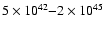 erg/s and peaks around 1044 erg/s (see Fig. 5,
dashed line). The number of QSO 2 candidates, therefore, is very sensitive to
the dividing line between low- and high-luminosity AGN, which is clearly
arbitrary and cosmology dependent. For example, if one defines as QSO 2 all
sources with
erg/s and peaks around 1044 erg/s (see Fig. 5,
dashed line). The number of QSO 2 candidates, therefore, is very sensitive to
the dividing line between low- and high-luminosity AGN, which is clearly
arbitrary and cosmology dependent. For example, if one defines as QSO 2 all
sources with
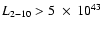 erg/s, a value only a factor of 2 below the commonly used one and corresponding to the break in the AGN X-ray
luminosity function (Norman et al. 2002), the number of such
sources increases by
erg/s, a value only a factor of 2 below the commonly used one and corresponding to the break in the AGN X-ray
luminosity function (Norman et al. 2002), the number of such
sources increases by  .
We also note that, based on the rms
around the Fiore et al. (2003) correlation, the number of QSO 2
candidates fluctuates in the 13-54 region. The number of type 2 AGN, on
the other hand, can only increase, as all our candidates have estimated
.
We also note that, based on the rms
around the Fiore et al. (2003) correlation, the number of QSO 2
candidates fluctuates in the 13-54 region. The number of type 2 AGN, on
the other hand, can only increase, as all our candidates have estimated
 .
.
It is interesting that all candidates with
have estimated X-ray
power
 erg/s, and therefore all qualify as AGN. Some
previously known sources, however, do have X-ray powers below this value (see
Sect. 6.1).
erg/s, and therefore all qualify as AGN. Some
previously known sources, however, do have X-ray powers below this value (see
Sect. 6.1).
As expected, being still unidentified, our sources are very faint: their
median ACS i magnitude is 25.5, which corresponds to  (compare this to the
  typical of the CDF-S sources with redshift
determination). The QSO 2 candidates are even fainter, with median i magnitude 26.3 (
typical of the CDF-S sources with redshift
determination). The QSO 2 candidates are even fainter, with median i magnitude 26.3 (
 ).
).
It is important to notice that 6 of the 21 sources in Table 2 have
actually been observed by Szokoly et al. (2004, see their Fig. 5)
but either their spectrum is featureless (4 sources) or the continuum is so
weak that no extraction could be made (2 sources).
5.1 Testing our estimated X-ray powers
To check the reliability of our estimated X-ray powers we compared the
predicted and observed luminosities for the already known sources. The Fiore
et al. (2003) correlation is valid for non-type 1 AGN and galaxies
so we did the comparison for these sources. Namely, we excluded the type 1
sources from the Szokoly et al. (2004) catalogue and the sources
with broad lines (type "B'') in Barger et al. (2003). Moreover, we
only considered sources with quality flag  in the former catalogue
and excluded objects with less secure redshifts (type "s'') in the latter, to
have reliable redshifts and therefore powers. This leaves us with 122
objects. For these, we find that
in the former catalogue
and excluded objects with less secure redshifts (type "s'') in the latter, to
have reliable redshifts and therefore powers. This leaves us with 122
objects. For these, we find that
 ,
where the slope is the mean ordinary least-squares slope
(Isobe et al. 1990). The mean values of the estimated (
,
where the slope is the mean ordinary least-squares slope
(Isobe et al. 1990). The mean values of the estimated (
 )
and observed (
)
and observed (
 )
luminosities, are consistent. This shows that our
method works for non-type 1 AGN and can then be safely applied to optically
unidentified but absorbed sources.
)
luminosities, are consistent. This shows that our
method works for non-type 1 AGN and can then be safely applied to optically
unidentified but absorbed sources.
It is tempting to use our estimated X-ray powers together with the observed
fluxes to derive redshifts for our type 2 candidates. We can first check how
reliable these are by comparing them with the spectroscopic redshifts
available for the known non-type 1 AGN described above. We follow standard
procedures (see, e.g., Mobasher et al. 2004) and quantify the
reliability of the estimated redshifts,
 ,
by measuring the
fractional error for each galaxy,
,
by measuring the
fractional error for each galaxy,
 .
We find a median error,
.
We find a median error,
 ,
an rms scatter,
,
an rms scatter,
 ,
and a rate of
"catastrophic'' outliers,
,
and a rate of
"catastrophic'' outliers,  ,
defined as the fraction of the full sample
that has
,
defined as the fraction of the full sample
that has
 ,
,
 .
Clipping these outliers gives
.
Clipping these outliers gives
 and
and
 .
For comparison,
Mobasher et al. (2004) have used extensive multiwavelength
photometric data to estimate photometric redshifts for a sample of 434 galaxies with spectroscopic redshifts in the CDF-S. They find
.
For comparison,
Mobasher et al. (2004) have used extensive multiwavelength
photometric data to estimate photometric redshifts for a sample of 434 galaxies with spectroscopic redshifts in the CDF-S. They find
 ,
,
and
,
,
and
 ,
depending on the subsample considered. Excluding the outliers they find values
of
,
depending on the subsample considered. Excluding the outliers they find values
of
 .
Given the simplicity of our method, these
results are certainly encouraging and show that our estimates should at least
provide a rough idea of the redshifts at which we might expect our sources to
be.
.
Given the simplicity of our method, these
results are certainly encouraging and show that our estimates should at least
provide a rough idea of the redshifts at which we might expect our sources to
be.
Applying this method to our type 2 AGN candidate list we find a mean of
 (median 2.6). The QSO 2 have,
as expected, significantly higher estimated redshifts
(median 2.6). The QSO 2 have,
as expected, significantly higher estimated redshifts
 compared to
 for the
non-QSO candidates.
for the
non-QSO candidates.
We can also use the ACS four band photometry to constrain the redshifts of our
sources. Cristiani et al. (2004) have discussed a set of four
optical criteria using the i-z, B-V, and V-i colours (a variation of the
"B-dropout'' technique) to select AGN in the redshift range
 .
By applying the same criteria to our candidates we find 9 such
sources. Their average estimated redshift is
.
By applying the same criteria to our candidates we find 9 such
sources. Their average estimated redshift is
 ,
and all but one sources have
,
and all but one sources have
 .
Again, this
shows that our estimated redshifts are, overall, relatively robust.
.
Again, this
shows that our estimated redshifts are, overall, relatively robust.
Table 3:
B dropouts.
These sources are listed in Table 3, which gives the GOODS ID in
Col. 1, the ACS i magnitude in Col. 2, followed by the i-z, V-iand B-V colours (all in the AB system) in Cols. 3-5.
![\begin{figure}
\par\includegraphics[width=5.8cm,clip]{alex50.ps}\includegraphics...
...m,clip]{alex268.ps}\includegraphics[width=5.8cm,clip]{alex272.ps}
\end{figure}](/articles/aa/full/2004/35/aa1153/Timg89.gif) |
Figure 2:
CDF-S Cutouts. B, V, i, and z ACS image cutouts are
displayed for all the type 2 AGN candidate in the CDF-S. Each image is
 in size, with north up and east to the left. The
Alexander identification number is shown in the top left of each panel, and
the circles drawn on the i-band images indicate the Alexander X-ray
positions, with the radius indicating the 90
in size, with north up and east to the left. The
Alexander identification number is shown in the top left of each panel, and
the circles drawn on the i-band images indicate the Alexander X-ray
positions, with the radius indicating the 90 positional error. The (black
and white) square symbols indicate the positions of the GOODS source which
have been matched to the X-ray positions. The X symbols indicate the positions
of any corresponding sources in the Szokoly catalogue.
positional error. The (black
and white) square symbols indicate the positions of the GOODS source which
have been matched to the X-ray positions. The X symbols indicate the positions
of any corresponding sources in the Szokoly catalogue. |
| Open with DEXTER |
![\begin{figure}
\par\includegraphics[width=5.2cm,clip]{alex24.ps}\includegraphics...
...s}\includegraphics[width=5.2cm,clip]{alex486.ps}\hspace*{2.7cm}}
\end{figure}](/articles/aa/full/2004/35/aa1153/Timg90.gif) |
Figure 3:
CDFN Cutouts. B, V, i, and z ACS image cutouts are displayed for all the type 2 AGN candidate in the CDFN.
Each image is
in size, with north up
and east to the left. The Alexander identification number is
shown in the top left of each panel, and the circles drawn on
the i-band images indicates the Alexander X-ray positions, with
the radius indicating the  positional error.
The (black and white) square symbols indicate the positions of the
GOODS sources which have been
matched to the X-ray positions. positional error.
The (black and white) square symbols indicate the positions of the
GOODS sources which have been
matched to the X-ray positions. |
| Open with DEXTER |
Out of the 9 QSO 2 previously known (see Sect. 6), our method has
rediscovered them all as type 2 AGN, 8/9 with
 erg/s (the ninth one having
 erg/s). Out of the 29 type 2 AGN with
L2 - 8 > 1042 erg/s in the
Szokoly et al. (2004) catalogue, 28 have
erg/s and therefore fulfil our selection criteria, while the last one is
barely below with
erg/s). Out of the 29 type 2 AGN with
L2 - 8 > 1042 erg/s in the
Szokoly et al. (2004) catalogue, 28 have
erg/s and therefore fulfil our selection criteria, while the last one is
barely below with
 erg/s.
During the completion of this work three redshift databases covering the CDF-S
and HDF-N became public. Namely: the ESO/GOODS FORS2 spectroscopy data
(Vanzella et al. 2004), the VIMOS VLT Deep Survey
(VVDS; Le Fèvre et al. 2004) and the Team Keck Treasury Redshift Survey (TKRS;
Wirth et al. 2004). We cross-matched our
candidate list with these surveys using the AVO prototype, finding only one
match, namely GOODS J123556.10+621219.6, with a quite featureless
spectrum and redshift
z = 0.9585 (our estimated redshift based on its X-ray
power and flux is z = 0.93). Given the limits of the three surveys, that is
 ,
,
 ,
and
,
and
 respectively, this
is not surprising. The only match we found, in fact, is the brightest of our
northern candidates.
respectively, this
is not surprising. The only match we found, in fact, is the brightest of our
northern candidates.
Table 4:
Type 2 AGN candidates, UDF.
Image cutouts of the ACS  data centred on each of the new AGN type 2
candidates were generated using the AVO prototype. This was done by sending
requests to the Aladin image server which remotely extracts the required image
sections in the four bands from a database containing the GOODS data. The
hierarchical description of the ACS images in terms of the IDHA data model,
and advanced protocols for sending detailed requests to the server makes this
process more efficient and flexible than traditional image servers.
Figures 2 and 3 display
sections of the cutouts in all four bands for the
CDF-S and HDF-N respectively. Each image is shown with a linear grey-scale
over the range of minimum to maximum image values of the individual
image sections. The 90% error circle of the
Alexander et al. (2003) catalogue X-ray positions is overlaid on
the i band images (since our method used the i band), along with the GOODS catalogue position (black/white squares). The Szokoly et al.
(2004) optical positions (X symbols) are also shown for the CDF-S sources (Fig. 2). Note that in a few cases the position of
the GOODS optical counterpart is outside the X-ray 90% error circle. These
are still valid matches in terms of the distance/error parameter (see
Sect. 4.4), which limits matches to within the total
positional uncertainty which is 1.8 times larger than the 90% radius.
data centred on each of the new AGN type 2
candidates were generated using the AVO prototype. This was done by sending
requests to the Aladin image server which remotely extracts the required image
sections in the four bands from a database containing the GOODS data. The
hierarchical description of the ACS images in terms of the IDHA data model,
and advanced protocols for sending detailed requests to the server makes this
process more efficient and flexible than traditional image servers.
Figures 2 and 3 display
sections of the cutouts in all four bands for the
CDF-S and HDF-N respectively. Each image is shown with a linear grey-scale
over the range of minimum to maximum image values of the individual
image sections. The 90% error circle of the
Alexander et al. (2003) catalogue X-ray positions is overlaid on
the i band images (since our method used the i band), along with the GOODS catalogue position (black/white squares). The Szokoly et al.
(2004) optical positions (X symbols) are also shown for the CDF-S sources (Fig. 2). Note that in a few cases the position of
the GOODS optical counterpart is outside the X-ray 90% error circle. These
are still valid matches in terms of the distance/error parameter (see
Sect. 4.4), which limits matches to within the total
positional uncertainty which is 1.8 times larger than the 90% radius.
Our sources cover a large spectrum of morphologies, ranging from extended,
low-surface brightness to point-like. It is interesting to note, however, that
all QSO 2 candidates are point-like.
![\begin{figure}
\par\includegraphics[width=5.6cm,clip]{udf_alex201.ps}\par\includ...
...alex243.ps}\par\includegraphics[width=5.6cm,clip]{udf_alex255.ps}
\end{figure}](/articles/aa/full/2004/35/aa1153/Timg100.gif) |
Figure 4:
CDF-S UDF Cutouts. B, V, i, and z ACS image
cutouts are displayed for the type 2 AGN candidates that
fall within the area of the UDF. The (black and white) square
symbols indicate the positions of the UDF sources in the
UDF catalogue.The  symbols indicate the positions
of any corresponding sources in the Szokoly catalogue. symbols indicate the positions
of any corresponding sources in the Szokoly catalogue. |
| Open with DEXTER |
A number of sources also fall within the Hubble Ultra Deep Field (UDF;
Beckwith et al. 2004). The UDF provides extremely deep ACS Wide
Field Channel imaging (proposal IDs 9978 and 10 086) of a single
 field centred on 033239.0,
 (J2000) which lies within the GOODS CDF-S
field. Five of the absorbed sources fall within this field, and 3 of these
(A03 201, 243 and 255) are in our list of unclassified type 2 AGN candidates
(Table 2). For these sources we cross matched the X-ray positions with
the UDF version 1.0
i-band detected catalogues to find the UDF optical counterparts. We then
used the UDF i band magnitudes to estimate the X-ray power using the Fiore
et al. (2003) correlation as described above. The estimated X-ray
powers, and UDF i band magnitudes for these 3 sources are listed in Table 4 and UDF image cutouts overlaid with the UDF, Alexander et al. (2003), and Szokoly et al. (2004) positions are
shown in Fig. 4. Note that for one source, A03 243, we
find a different, fainter, optical counterpart than was found using the GOODS catalogue, resulting in a larger estimated X-ray power. Classically, one would
have solved this dilemma by obtaining a spectrum of both sources. However,
given the faintness of the two candidates (
(J2000) which lies within the GOODS CDF-S
field. Five of the absorbed sources fall within this field, and 3 of these
(A03 201, 243 and 255) are in our list of unclassified type 2 AGN candidates
(Table 2). For these sources we cross matched the X-ray positions with
the UDF version 1.0
i-band detected catalogues to find the UDF optical counterparts. We then
used the UDF i band magnitudes to estimate the X-ray power using the Fiore
et al. (2003) correlation as described above. The estimated X-ray
powers, and UDF i band magnitudes for these 3 sources are listed in Table 4 and UDF image cutouts overlaid with the UDF, Alexander et al. (2003), and Szokoly et al. (2004) positions are
shown in Fig. 4. Note that for one source, A03 243, we
find a different, fainter, optical counterpart than was found using the GOODS catalogue, resulting in a larger estimated X-ray power. Classically, one would
have solved this dilemma by obtaining a spectrum of both sources. However,
given the faintness of the two candidates (
 and 28.3), this is
unlikely to happen in the near future. (The two previously classified sources
that fall within the UDF are A03 245 (QSO-2) and 242 (AGN-1).)
and 28.3), this is
unlikely to happen in the near future. (The two previously classified sources
that fall within the UDF are A03 245 (QSO-2) and 242 (AGN-1).)
Note that none of our candidates have spectra obtained with
the ACS High Resolution Channel grism as part of the UDF observing
campaign.
6 Discussion
6.1 Previously known type 2 AGN
Table 5:
Previously Known Type 2 AGN, HDF-N.
We defined a sample of previously known type 2 AGN in the GOODS ACS fields as
follows. In the HDF-N, we selected absorbed (
)
sources without
broad lines (type "B'' in Barger et al. 2003) having X-ray power
L2-8 > 1042 erg/s (see Sect. 4.4). In the CDF-S we initially
selected sources with "AGN-2'' or "QSO-2'' classifications in Szokoly et al. (2004). We then applied the further criteria that
L2-8 >
1042 erg/s and
in order to be consistent with the HDF-N
sample. Successive power and  cuts exclude 2 and 3 sources respectively,
with a further 3 sources excluded because they have no counterpart in the
Alexander et al. (2003) catalogue (which is necessary for
consistent definitions of
and L2-8). (Note that differences
between our values and those listed by Szokoly et al. 2004,
can be explained by the different input catalogues produced by Giacconi et al.
2002 and Alexander et al. 2003.) These
definitions lead to a total of 79 known type 2 AGN (CDF-S: 35, HDF-N:
44). These are listed in Tables 5 and 6, which
give the Alexander et al. (2003) and Szokoly et al.
(2004) (for the CDF-S) IDs, redshift, hard X-ray power, and
notes. Only 9 of these sources can be classified as QSO 2 (
L2-8 > 1044 erg/s), 3 of which have poor redshift determinations (two
sources with type "s'' flags in Barger et al. 2003, and one source
with quality flag = 1 in Szokoly et al. 2004). We also note
that with a lower X-ray power cut of
cuts exclude 2 and 3 sources respectively,
with a further 3 sources excluded because they have no counterpart in the
Alexander et al. (2003) catalogue (which is necessary for
consistent definitions of
and L2-8). (Note that differences
between our values and those listed by Szokoly et al. 2004,
can be explained by the different input catalogues produced by Giacconi et al.
2002 and Alexander et al. 2003.) These
definitions lead to a total of 79 known type 2 AGN (CDF-S: 35, HDF-N:
44). These are listed in Tables 5 and 6, which
give the Alexander et al. (2003) and Szokoly et al.
(2004) (for the CDF-S) IDs, redshift, hard X-ray power, and
notes. Only 9 of these sources can be classified as QSO 2 (
L2-8 > 1044 erg/s), 3 of which have poor redshift determinations (two
sources with type "s'' flags in Barger et al. 2003, and one source
with quality flag = 1 in Szokoly et al. 2004). We also note
that with a lower X-ray power cut of
 erg/s the
number of QSO 2 increases to 13.
erg/s the
number of QSO 2 increases to 13.
Table 6:
Previously Known Type 2 AGN, CDF-S.
Figure 5 shows the X-ray power distribution for our new type 2 AGN candidates (dashed line), previously known type 2 AGN (solid line), and the
combined sample (dotted line). It is interesting to note how the distributions
are very different, with the already known type 2 AGN peaking around
 erg/s and declining for luminosities above
 erg/s, while our new candidates are rising in this range and peak
around
erg/s, while our new candidates are rising in this range and peak
around
 erg/s. To be more quantitative, while only 1/5 of already known type 2 AGN have
 ,
3/4 of our candidates are above this value. This difference is easily
explained by our use of the X-ray-to-optical flux ratios to estimate X-ray
powers and by the fact that our candidates are on average 3 mag
fainter than previously known sources. Our method is then filling a gap in the
luminosity distribution, which becomes almost constant in the range
,
3/4 of our candidates are above this value. This difference is easily
explained by our use of the X-ray-to-optical flux ratios to estimate X-ray
powers and by the fact that our candidates are on average 3 mag
fainter than previously known sources. Our method is then filling a gap in the
luminosity distribution, which becomes almost constant in the range
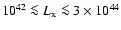 erg/s. This also explains the fact that
the number of QSO 2 candidates we find is 3 times larger than the
previously known ones.
erg/s. This also explains the fact that
the number of QSO 2 candidates we find is 3 times larger than the
previously known ones.
Conversely the fluxes of the already known QSO 2 reach
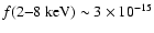 erg cm-2 s-1, while our new QSO 2 candidates go
down to the fainter limit of
erg cm-2 s-1, while our new QSO 2 candidates go
down to the fainter limit of
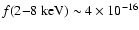 erg cm-2 s-1. This is explained by the much fainter optical magnitudes
we are probing with our method which, for a given X-ray-to-optical flux ratio,
translate into fainter X-ray fluxes as well.
erg cm-2 s-1. This is explained by the much fainter optical magnitudes
we are probing with our method which, for a given X-ray-to-optical flux ratio,
translate into fainter X-ray fluxes as well.
By going fainter we are also probing the type 2 AGN population at higher
redshifts. While our estimated redshift is
(median 2.6), previously known type 2 AGN have
 (median 0.9). For QSO 2 we find
(median 3.5), as compared to
(median 0.9). For QSO 2 we find
(median 3.5), as compared to
 (median 2.6).
![\begin{figure}
\par\includegraphics[width=8.3cm,clip]{1153fig5.eps}
\end{figure}](/articles/aa/full/2004/35/aa1153/Timg116.gif) |
Figure 5:
The X-ray power distribution for our new type 2 AGN candidates
(dashed line), previously known type 2 AGN (solid line), and
the sum of the two populations (dotted line). QSO 2 are defined,
somewhat arbitrarily, as having
 erg/s. erg/s. |
| Open with DEXTER |
6.2 Total number of type 2 AGN
We find a total of 147 type 2 AGN in the GOODS ACS area, 79 of which were
already known. This corresponds to
 of the 546 sources in the
Alexander et al. (2003) catalogue (
of the 546 sources in the
Alexander et al. (2003) catalogue (
 including
the previously known sources only). As regards QSO 2, the total number is 40,
only 9 of which were previously known. Our method has therefore more than
quadrupled the number of such sources in the GOODS ACS fields. These represent
including
the previously known sources only). As regards QSO 2, the total number is 40,
only 9 of which were previously known. Our method has therefore more than
quadrupled the number of such sources in the GOODS ACS fields. These represent
 of all (546) X-ray sources (the previously known QSO 2 make up
 ).
).
Note that all of these sources satisfy the commonly adopted definition of
absorbed source discussed above. In fact, Fig. 12 of Szokoly et al.
(2004) shows that
corresponds to
cm-2, for an intrinsic
 ,
for
,
for  .
The lowest redshift for previously known type 2 AGN is 0.4, while the
lowest estimated redshift for our type 2 candidates is 0.9. The typical and redshifts for our sources imply that we are dealing with
.
The lowest redshift for previously known type 2 AGN is 0.4, while the
lowest estimated redshift for our type 2 candidates is 0.9. The typical and redshifts for our sources imply that we are dealing with
 and
and 
 cm-2 for the
known and candidate sources respectively.
cm-2 for the
known and candidate sources respectively.
X-ray obscuration can be also present in a small fraction of broad-lined AGN. Perola et al. (2004, and references therein) find this to
be the case in  of their sources, with estimated
 cm-2. As discussed in the previous paragraph, these
sources are then likely to be at relatively low redshift. Therefore,
contamination by type 1 AGN in our sample is expected to be negligible.
cm-2. As discussed in the previous paragraph, these
sources are then likely to be at relatively low redshift. Therefore,
contamination by type 1 AGN in our sample is expected to be negligible.
6.3 The surface density of QSO 2
Table 7:
QSO 2 surface density.
The detection of faint type 2 AGN candidates and the careful assessment of the
previously known such sources in the two GOODS fields allow us to put strong
constraints on the surface density of type 2 sources, and in particular on
that of QSO 2. We use a value for the  -band coverage of 365 arcmin
 deg2 (Giavalisco et al. 2004a).
Due to the variable sensitivity of the Chandra ACIS-I detector across the field of
view, the area in which fainter X-ray sources could be detected is smaller
than that for brighter sources. In other words, the sky coverage is not
uniform at all fluxes. Figure 5 of Giacconi et al. (2002) and
Fig. 19 of Alexander et al. (2003), however, show that the effect
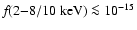
is strong only at relatively small fluxes. For example, for both CDF-S and
HDF-N the effective area decreases in the hard band, for which this effect is
strongest, by  only for
 erg cm-2 s-1.
To better quantify the magnitude of this correction we evaluated the sky
coverage for the combined GOODS fields by simply scaling the two sky coverages
so that the maximum area for each field was equal to half the total GOODS area, summing then up the two areas. This works only as a first approximation
and slightly overestimates the correction since the GOODS ACS fields are at
the centre of the Chandra fields and therefore deeper than average in the
X-ray band. In other words, the sky coverage should be re-computed as its
shape would change, with a larger area accessible at fainter fluxes and
therefore a smaller correction than we estimate. In any case, under our
assumptions we find that the correction is within the Poisson range,
and therefore within the statistical uncertainties, for
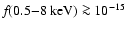 erg cm-2 s-1. Our conservative approach is then to not
to take the sky coverage into account and limit ourselves to X-ray
erg cm-2 s-1. Our conservative approach is then to not
to take the sky coverage into account and limit ourselves to X-ray
 erg cm-2 s-1. This means that our values are actually lower limits, although the real surface densities should not be more than
larger.
erg cm-2 s-1. This means that our values are actually lower limits, although the real surface densities should not be more than
larger.
Table 7 gives the QSO 2 surface density for four flux limits,
splitting the contribution into known and candidate sources for the full 0.5-8 keV band. (The counts in the hard band are not very different,
since we are dealing with absorbed sources, with the total numbers
changing to 33 (from 34) and 8 (from 10) for the first and third flux limit
respectively.)
These numbers can be compared with recent estimates and predictions. Perola et al. (2004) find a surface density of highly obscured QSO, which
they define as having
L2-10 > 1044 erg/s and
cm-2, 48 deg-2 for
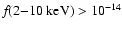 erg cm-2 s-1, consistent with our value. At lower fluxes the situation
is different. For example, for
erg cm-2 s-1, consistent with our value. At lower fluxes the situation
is different. For example, for
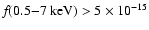 erg cm-2 s-1 Gandhi et al. (2004) quote an estimated value >3 deg-2 and possibly higher than 10 deg-2 and a predicted value
from their model of 19 deg-2. We find a density
erg cm-2 s-1 Gandhi et al. (2004) quote an estimated value >3 deg-2 and possibly higher than 10 deg-2 and a predicted value
from their model of 19 deg-2. We find a density  deg-2,
that is a factor
deg-2,
that is a factor  larger than their estimate and 5 times larger
than their prediction. Already known sources make up
larger than their estimate and 5 times larger
than their prediction. Already known sources make up  of our total
value, so this high density is clearly not attributable only to our new
candidates. We do note that 5 out of the 7 previously known QSO 2 come from
the paper by Szokoly et al. (2004), which appeared only recently
and could not be accounted for by Gandhi et al. (2004). For the same
flux limit and
of our total
value, so this high density is clearly not attributable only to our new
candidates. We do note that 5 out of the 7 previously known QSO 2 come from
the paper by Szokoly et al. (2004), which appeared only recently
and could not be accounted for by Gandhi et al. (2004). For the same
flux limit and
 erg/s these authors predict a
surface density
erg/s these authors predict a
surface density  deg-2, while we find 5 sources (3 of them
already known), which implies a density
49+33-21 deg-2. The
decrease in space density at high luminosity is therefore much less than
predicted by their model, namely only a factor 2 instead of 6.
deg-2, while we find 5 sources (3 of them
already known), which implies a density
49+33-21 deg-2. The
decrease in space density at high luminosity is therefore much less than
predicted by their model, namely only a factor 2 instead of 6.
At even fainter fluxes, Gandhi et al. (2004) quote a value from
their model of 35 deg-2 above
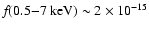 erg cm-2 s-1, while we find a density
  deg-2, that is a factor
  larger than their prediction.
The population synthesis model of Gilli et al.
(2001, and private communication) predicts 16 obscured QSO with
intrinsic luminosity
erg/s,
cm-2, and z > 3 in the 1 Ms CDF-S. We find 2 known plus 7 candidate sources above these redshift and power limits with
.
According to Fig. 12 of Szokoly et al. (2004) at  an
an
 cm-2 corresponds to
 for an
intrinsic
,
which means that our definition is more
restrictive. Considering also that the southern GOODS ACS area is
smaller than the CDF-S area, there are strong indications that our
number might be a very solid lower limit to such sources and that therefore
our findings are not inconsistent with the numbers predicted by Gilli et al. (2001).
for an
intrinsic
,
which means that our definition is more
restrictive. Considering also that the southern GOODS ACS area is
smaller than the CDF-S area, there are strong indications that our
number might be a very solid lower limit to such sources and that therefore
our findings are not inconsistent with the numbers predicted by Gilli et al. (2001).
As mentioned in Sect. 5, the number of our QSO 2 candidates
depends on the
 correlation of
Fiore et al. (2003), which has an rms of 0.5 dex in X-ray
power. However, even if we consider the worst case scenario in which all
our estimated X-ray powers are too large by 0.5 dex the number of QSO 2
candidates for the four flux limits in Table 7 are 13, 8, 2, and 1 respectively. In other words, our total densities decrease, at worst, by
correlation of
Fiore et al. (2003), which has an rms of 0.5 dex in X-ray
power. However, even if we consider the worst case scenario in which all
our estimated X-ray powers are too large by 0.5 dex the number of QSO 2
candidates for the four flux limits in Table 7 are 13, 8, 2, and 1 respectively. In other words, our total densities decrease, at worst, by  at the lowest fluxes, and are basically unchanged at larger fluxes.
The resolved fraction of the X-ray background due to QSO 2 down to
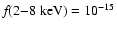 erg cm-2 s-1 is estimated
to be
erg cm-2 s-1 is estimated
to be
 .
We have used here the value of the total X-ray
background measured by UHURU and HEAO-1 (Marshall et al.
1980) and the uncertainties reflect the rms of
the Fiore et al. (2003) correlation (the Poissonian error is
even smaller). Note that given the relatively small area of the GOODS fields we are missing the bright end of the number counts. In fact,
only four of our sources have
.
We have used here the value of the total X-ray
background measured by UHURU and HEAO-1 (Marshall et al.
1980) and the uncertainties reflect the rms of
the Fiore et al. (2003) correlation (the Poissonian error is
even smaller). Note that given the relatively small area of the GOODS fields we are missing the bright end of the number counts. In fact,
only four of our sources have
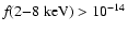 erg cm-2 s-1 and these reach only
 erg cm-2 s-1. This fact, the discussion above and the points
detailed in the next section, all mean that our value has to be
regarded as a robust lower limit.
erg cm-2 s-1. This fact, the discussion above and the points
detailed in the next section, all mean that our value has to be
regarded as a robust lower limit.
In this paper we have employed a statistical method to identify very faint
type 2 AGN. We had also to rely on an empirical technique to estimate the
X-ray powers, which were needed to make sure that the sources we are dealing
with have AGN-like outputs. As such, we can only provide a list of candidates
and not firm classifications. This was obviously expected, as the great
majority of our candidates are so faint that even the largest telescopes
presently available would require extremely long exposures to secure a decent
spectrum.
However, we believe that our method is robust, as shown by the various checks
we have performed. Importantly, we have been very conservative in our
estimates of the number of type 2 AGN candidates and the surface densities we
have estimated need to be considered lower limits (modulo what discussed in
the previous paragraph), for the following four reasons: 1. our selection
criterion for absorbed sources (
)
will mistakenly discard some
high-z type 2 sources (Sect. 4.1); 2. the same criterion is also more
restrictive than the commonly used one based on
(Sect. 6.2); 3. the X-ray powers for previously known sources have not been
corrected for absorption, which means more sources could be above the QSO 2 limit (Sect. 4.3); and finally, 4. sky coverage effects, once
properly taken into account, will reduce the available area at smaller X-ray
fluxes and therefore increase the source surface density (Sect. 6.3).
As noted above, a remaining source of uncertainty with the newly discovered
sample is the reliance on an empirical technique in the determination of the
X-ray power of the objects.
In Sect. 5.1 we noted how the 4 colour ACS photometric data have been
used to estimate redshifts for a number of objects in a restricted range.
Future work will enable the use of the 4 band ACS plus IR (VLT/ISAAC and
Spitzer) photometry to determine photometric redshifts over the full GOODS field. VO technologies are to be employed to facilitate this work. Upgrades to
the AVO capability will include the provision of a "redshift-determination''
service, which will automate the generation of point spread function matched
multi-band input photometric catalogues via the use of AstroGrid's (Walton
et al. 2003) ACE (Astronomical Catalogue Extractor)
service (a Web service providing access to the SExtractor application, Bertin
& Arnouts 1996), and feed these into a range of photometric
redshift determination techniques (e.g., Bayesian prior method, Bpz, Benítez 2000; the neural network technique, ANNz, Collister & Lahav
2004; and Hyperz, Bolzonella et al.
2000).
It is necessary to include the IR data in order to obtain
reliable photometric redshifts, and with the
additional photometric bands, the effects of possible dust extinction
will also be identifiable (Rowan-Robinson 2003).
We have used Virtual Observatory tools to identify obscured AGN much fainter
than previously known ones, going beyond what is currently possible using the
"classical'' approach of classifying sources by taking spectra of them even
using the largest telescopes available today. The fact that we have obtained
scientifically useful and cutting-edge results is proof that VO tools have
evolved beyond the demonstration level to become respectable research
tools. The VO is already enabling astronomers to reach into new areas of
parameter space with relatively little effort.
Our main results can be summarized as follows:
- 1.
- By employing publicly available, high-quality X-ray and optical data we
have discovered 68 type 2 AGN candidates in the two GOODS fields. Their X-ray
powers have been estimated by using a previously known correlation between
X-ray luminosity and X-ray-to-optical flux ratio. Thirty-one of our candidates
have high luminosity (
erg/s) and therefore
qualify as QSO 2, that is optically obscured quasars. Based on their derived
X-ray powers, our candidates are likely to be at relatively high redshifts, ,
with the QSO 2 at .
- 2.
- We have tested our method and results extensively and find them to be
very robust. In particular: a) our approach recovers most (
 )
of the
previously known type 2 AGN in the GOODS fields; b) the X-ray power estimates
agree very well with those derived from spectroscopic redshifts for
the non-type 1 AGN in the GOODS fields; c) the redshifts derived from our
estimated powers are consistent with those measured for previously known
non-type 1 AGN; d) the spectrum of our brightest northern candidate, recently
made public as part of the Team Keck Treasury Redshift Survey, confirms our
type 2 classification as it is basically featureless, with a measured redshift
extremely close to our estimate.
)
of the
previously known type 2 AGN in the GOODS fields; b) the X-ray power estimates
agree very well with those derived from spectroscopic redshifts for
the non-type 1 AGN in the GOODS fields; c) the redshifts derived from our
estimated powers are consistent with those measured for previously known
non-type 1 AGN; d) the spectrum of our brightest northern candidate, recently
made public as part of the Team Keck Treasury Redshift Survey, confirms our
type 2 classification as it is basically featureless, with a measured redshift
extremely close to our estimate.
- 3.
- By going 3 mag fainter than previously known type 2 AGN we
are sampling a region of redshift - power space so far unreachable with
classical methods. Our method brings to 40 the number of QSO 2 in the
GOODS fields, an improvement of a factor 4 when compared to the 9 such
sources previously known. The relatively large QSO 2 number density we derive
(330 deg-2 for
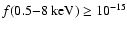 erg cm-2 s-1,
of which is made up of already known sources) suggests
that its value at faint flux limits has been underestimated.
erg cm-2 s-1,
of which is made up of already known sources) suggests
that its value at faint flux limits has been underestimated.
For the handful of our candidates with  spectroscopy with a
class 8-10 m telescope is still within reach, albeit with relatively
long (10 h) exposure times. We plan to follow these up and
confirm (or refute) their classification in the near future.
spectroscopy with a
class 8-10 m telescope is still within reach, albeit with relatively
long (10 h) exposure times. We plan to follow these up and
confirm (or refute) their classification in the near future.
In closing we note that this paper represents the first significant published
science result that has been fully enabled via end-to-end use of VO tools and
systems.
VO initiatives are in their early stages. Significant progress is being made
both by the AVO and other national VO projects. Construction of a truly
pervasive system is beginning to provide the end user access to a powerful
combination of data access, applications embedded within user workflows,
running over high speed networks on powerful compute resources. Early use,
exploiting a prototype system in the USA, constructed by the US-VO
project to simplify the cross matching of
Two Micron All Sky Survey and Sloan Digital Sky Survey source catalogues has
enabled Berriman et al. (2003) to discover a small number of
hitherto undiscovered Brown Dwarf candidates. Their work demonstrated
possibilities, but did not alter the scientific understanding of that
particular problem.
In this paper we have shown how, even with the AVO's early prototype, enough
capability and access to data is available to make the scientific mining of
the, in this case GOODS, data significantly easier for the "general''
astronomer. This is because gains in interoperability simplify the acquisition
of the data, and enable quick interoperation of a number of common, but
computationally intensive, tasks such as cross matching and multi layer
visualisation of both image and catalogue data.
With the rapid evolution of the VO, science discovery will be routinely
performed using VO techniques, an early example of which is described here.
The AVO prototype used in this paper is freely available for
download.
Acknowledgements
We thank Fabrizio Fiore for providing the data on which the X-ray
power - X-ray-to-optical flux ratio correlation was based, Roberto
Gilli, Vincenzo Mainieri, and Paolo Tozzi for useful
discussions, Sebastien Derriere for assistance with the false match
rate estimates, and the AVO team for their superb work, without which
this paper would have not been possible. Finally, a sincere "thank
you'' to the many people who have produced the data on which this
paper is based, particularly the GOODS, CDF-S, and Penn State
Teams. This research has made use of the CDS Vizier catalogue tool,
SIMBAD and Aladin sky atlas services.
Appendix A: False match estimate
We estimated the number of false matches using the formalism described
in Derriere (2001). The expected total number of matches D,
for N1 objects with positional uncertainty
against a uniformly
distributed set of objects with density  is:
is:
![$\displaystyle D(d,N_1,\lambda,\sigma,N)=
N_1\Phi(d,\lambda)+N\Phi(d,\lambda)\le...
...\sigma^2}{2\pi
\lambda\sigma^2}\exp\left(-\frac{d^2}{2\sigma^2}\right)-1\right]$](/articles/aa/full/2004/35/aa1153/img173.gif) |
|
|
(A.1) |
where d is the distance between matches,
 is the 2-d Poisson density function and N is the number of objects with a true
counterpart. D may also be expressed a sum of three components,
is the 2-d Poisson density function and N is the number of objects with a true
counterpart. D may also be expressed a sum of three components,
 the number of true matches,
the objects with a true partner but not incorrectly assigned and
the number of true matches,
the objects with a true partner but not incorrectly assigned and  the number of objects that do
not have a counterpart but have been matched.
the number of objects that do
not have a counterpart but have been matched.
Using our known values of N1: the number of absorbed sources (203),
:
the optical source density of the GOODS catalogues
(0.0469 arcsec-2), and :
the median positional error of the X-ray
positions of the absorbed sources (0.31
)
we vary N to perform a
maximum likelihood fit of the expected distribution of matches D to the
observed histogram of distances between closest match optical and X-ray
sources out to the initial 3.5
threshold radius. The best fit occurs
for N=160. Figure A.1 shows the histogram of distances between
closest match optical and X-ray sources overlaid with the best fitting model.
![\begin{figure}
\par\includegraphics[width=8cm,clip]{1153fig6.ps}
\end{figure}](/articles/aa/full/2004/35/aa1153/Timg181.gif) |
Figure A.1:
The histogram of distances between closest match optical and X-ray
sources overlaid with the best fitting model. |
Integrating D and
out to 1.25
we find that 92% of the
matches out to this radius are expected to be true according to the model,
making our false match fraction 8%. Note that this approach neglects
clustering, which would slightly increase this value.
We also estimated the number of false matches by comparing the number of X-ray
to optical matches we find using the correct coordinates, to the number of
matches we find when a shift (of 20
much larger than the typical
match radius and the spacing between optical sources) is applied to the X-ray
coordinates. Within 1.25
we find 188 matches and 38 matches when the
coordinates are shifted. Our selection of real matches however, also included
the distance/error criterion which means that a number of matching sources
within 1.25
of the X-ray source were discarded. This criterion should
also be taken into consideration when estimating the rate of false matches. We
estimate this effect on the false match rate by calculating the rate of
optical sources within 1.25
of the real X-ray position which have
distance/error >1 (10), and then subtract this from the rate of false matches we
find in the offset cross-match. Therefore the false match fraction using this
method should be (38-10)/188 = 15%.
The fraction of false matches should then be in the range  .
.
- Alexander, D.
M., Bauer, F. E., Brandt, W. N., et al. 2003, AJ, 126, 539 [NASA ADS] (In the text)
- Barger, A. J.,
Cowie, L. L., Capak, P., et al. 2003, AJ, 126, 632 [NASA ADS] (In the text)
- Beckwith, S. V.
W., et al. 2004, in preparation
(In the text)
- Benítez, N.
2000, ApJ, 536, 571 [NASA ADS] (In the text)
- Berriman, B.,
Kirkpatrick, D., Hanisch, R., Szalay, A., & Williams, R. 2003,
Large Telescopes and Virtual Observatory: Visions for the future,
25th Meet. of the IAU, Joint Discussion 8, 17 July, Sydney,
Australia, in press
(In the text)
- Bertin, E., &
Arnouts, S. 1996, A&A, 117, 393 [NASA ADS] (In the text)
- Bolzonella,
M., Miralles, J.-M., & Pello, R. 2000, A&A, 363, 476 [NASA ADS] (In the text)
- Bonnarel,
F., Fernique, P., Bienaymé, O., et al. 2000, A&AS, 143,
33 [NASA ADS] (In the text)
- Cohen, J. G. 2003,
ApJ, 598, 288 [NASA ADS] (In the text)
- Collister, A.
A., & Lahav, O. 2004, PASP, 116, 345 [NASA ADS] (In the text)
- Comastri, A.,
Fiore, F., Vignali, C., et al. 2001, MNRAS, 327, 781 [NASA ADS] (In the text)
- Cristiani,
S., Alexander, D. M., Bauer, F., et al. 2004, ApJ, 600, L119 [NASA ADS] (In the text)
- Derriere, S.
2001, Ph.D. Thesis (Annexe B)
(In the text)
- Fiore, F., Brusa, M.,
Cocchia, F., et al. 2003, A&A, 409, 79 [EDP Sciences] [NASA ADS] (In the text)
- Forman, W., Jones,
C., & Tucker, W. 1994, ApJ, 429, 77 [NASA ADS] (In the text)
- Gandhi, P.,
Crawford, C. S., Fabian, A. C., & Johnstone, R. M. 2004, MNRAS,
348, 529 [NASA ADS] (In the text)
- Gehrels, N. 1986,
ApJ, 303, 336 [NASA ADS] (In the text)
- Giacconi, R.,
Zirm, A., Wang, J. X., et al. 2002, ApJS, 139, 369 [NASA ADS] (In the text)
- Giavalisco, M.,
Ferguson, H. C., Koekemoer, A. M., et al. 2004a, ApJ, 600, L93 [NASA ADS] (In the text)
- Giavalisco, M.,
& the GOODS Team 2004b, in preparation
(In the text)
- Gilli, R., Salvati,
M., & Hasinger, G. 2001, A&A, 366, 407 [EDP Sciences] [NASA ADS] (In the text)
- Isobe, T., Feigelson,
E. D., Akritas, M. G., & Babu, G. J. 1990, ApJ, 364, 104 [NASA ADS] (In the text)
- Jaffe, W.,
Meisenheimer, K., Röttgering, H. J. A., et al. 2004, Nature,
429, 47 [NASA ADS] [CrossRef] (In the text)
- Le Fèvre,
O., Vettolani, P., Paltani, S., et al. 2004, A&A,
submitted
(In the text)
- Maccacaro,
T., Gioia, I. M., Wolter, A., Zamorani, G., & Stocke, J. T.
1988, ApJ, 326, 680 [NASA ADS] (In the text)
- Marshall, F.
E., Boldt, E. A., Holt, S. S., et al. 1980, ApJ, 235, 4 [NASA ADS] (In the text)
- Mobasher, B.,
Idzi, R., Benítez, N., et al. 2004, ApJ, 600, L167 [NASA ADS] (In the text)
- Moran, E. C.,
Filippenko, A. V., & Chornock, R. 2002, ApJ, 579, L71 [NASA ADS] (In the text)
- Norman, C.,
Hasinger, G., Giacconi, R., et al. 2002, ApJ, 571, 218 [NASA ADS] (In the text)
-
Ochsenbein, F., Bauer, P., & Marcout, J. 2000, A&AS, 143,
23 [NASA ADS] (In the text)
- Perola, G. C.,
Puccetti, S., Fiore, F., et al. 2004, A&A, 421, 491 [EDP Sciences] [NASA ADS] (In the text)
- Rowan-Robinson, M.
2003, MNRAS, 345, 819 [NASA ADS] (In the text)
- Shapley, A.,
Fabbiano, G., & Eskridge, P. B. 2001, ApJS, 137, 139 [NASA ADS] (In the text)
- Szokoly, G. P.,
Bergeron, J., Hasinger, G., et al. 2004, ApJS, in press
[arXiv:astro-ph/0312324]
(In the text)
- Urry, C. M., &
Padovani, P. 1995, PASP, 107, 803 [NASA ADS] (In the text)
- Vanzella, E.,
et al. 2004, in preparation
(In the text)
- Walton, N. A.,
Lawrence, A., & Linde, A. E. 2003, ASASS, 12, 25 [NASA ADS] (In the text)
- Wirth, G. D.,
Willmer, C. N. A., Amico, P., et al. 2004, AJ, 127, 3121 [NASA ADS] (In the text)
- Zombeck, M. V.
1990, Handbook of Space Astronomy and Astrophysics (Cambridge
University Press)
Copyright ESO 2004
![\begin{figure}
\par\includegraphics[width=8.3cm,clip]{1153fig1.eps}
\end{figure}](/articles/aa/full/2004/35/aa1153/img46.gif)
![\begin{figure}
\par\includegraphics[width=5.8cm,clip]{alex50.ps}\includegraphics...
...m,clip]{alex268.ps}\includegraphics[width=5.8cm,clip]{alex272.ps}
\end{figure}](/articles/aa/full/2004/35/aa1153/img89.gif)
![\begin{figure}
\par\includegraphics[width=5.2cm,clip]{alex24.ps}\includegraphics...
...s}\includegraphics[width=5.2cm,clip]{alex486.ps}\hspace*{2.7cm}}
\end{figure}](/articles/aa/full/2004/35/aa1153/img90.gif)
![\begin{figure}
\par\includegraphics[width=5.6cm,clip]{udf_alex201.ps}\par\includ...
...alex243.ps}\par\includegraphics[width=5.6cm,clip]{udf_alex255.ps}
\end{figure}](/articles/aa/full/2004/35/aa1153/img100.gif)
![\begin{figure}
\par\includegraphics[width=8.3cm,clip]{1153fig5.eps}
\end{figure}](/articles/aa/full/2004/35/aa1153/img116.gif)
![\begin{figure}
\par\includegraphics[width=8cm,clip]{1153fig6.ps}
\end{figure}](/articles/aa/full/2004/35/aa1153/img181.gif)