A&A 421, 783-795 (2004)
DOI: 10.1051/0004-6361:20035778
F. K. Röpke1 - W. Hillebrandt2 - J. C. Niemeyer3
1 - Max-Planck-Institut für Astrophysik,
Karl-Schwarzschild-Str. 1, 85741 Garching, Germany
2 -
Max-Planck-Institut für Astrophysik,
Karl-Schwarzschild-Str. 1, 85741 Garching, Germany
3 -
Universität Würzburg,
Am Hubland, 97074 Würzburg, Germany
Received 1 December 2003 / Accepted 8 April 2004
Abstract
We investigate the interaction of thermonuclear flames in Type Ia supernova explosions with vortical flows by means of numerical simulations. In our study, we focus on
small scales, where the flame propagation is no longer dominated by the
turbulent cascade originating from large-scale effects. Here,
the flame propagation proceeds in the cellular burning regime,
resulting from a balance between the Landau-Darrieus instability and
its nonlinear stabilization. The
interaction of a cellularly
stabilized flame front with a vortical fuel flow is explored applying
a variety of fuel densities and strengths of the velocity
fluctuations. We find that the vortical flow can break up the cellular
flame structure if it is sufficiently strong. In this case the flame
structure adapts to the imprinted flow field. The transition from
the cellularly stabilized front to the flame structure dominated by
vortices of the flow proceeds in a smooth way. The implications of the
results of our simulations for Type Ia Supernova explosion models are
discussed.
Key words: stars: supernovae: general - hydrodynamics - instabilities - turbulence
In the canonical astrophysical model Type Ia supernovae (SNe Ia in the following) are associated with thermonuclear explosions of white dwarf (WD) stars (Hoyle & Fowler 1960). These WDs are composed of carbon and oxygen. Due to the high temperature sensitivity of the activation energy of carbon and oxygen burning, the reaction is confined to a very narrow region and propagates as a combustion wave. This defines a thermonuclear flame. The theoretical understanding of flame propagation in WDs provides the key to SN Ia explosion models with the effective flame velocity being the most important parameter. What are the phenomena that mediate the combustion wave? The answer to that question is given by the hydrodynamics of combustion. Conservation laws across the flame admit two fundamental modes of flame propagation: the detonation, in which the flame propagates due to shock waves, and the deflagration, which is based on microphysical transport phenomena such as heat conduction and species diffusion.
Flame propagation in the detonation mode is certainly the easiest to model. Here the flame propagation velocity with respect to the unburnt material is larger than the corresponding sound speed. Therefore the WD star has no time to expand prior to the incineration in this detonation model of SN Ia explosions and all the material is consumed at high densities resulting in ashes consisting solely of iron-peak elements (Arnett 1969). However, this is in conflict with observational spectra, which show strong indication of intermediate mass elements.
Consequently, the star has to expand considerably before it is processed by the thermonuclear flame. This is possible if flame propagation starts out in the deflagration mode, since here the microphysical transport processes lead to a subsonic flame velocity. In the present study, we refer to that deflagration model of SNe Ia. Moreover, underlying to our model is the so-called single-degenerate scenario, where the progenitor is a binary system with the WD accreting matter from the non-degenerate companion until it reaches the Chandrasekhar mass. At this point, thermonuclear reaction ignites near the center of the WD and propagates outward as a deflagration flame. For a review of SN Ia explosion models we refer to Hillebrandt & Niemeyer (2000).
In the framework of the deflagration model, recent large-scale SN Ia explosion models have been quite successful (Gamezo et al. 2003; Reinecke et al. 2002). Nevertheless, the determination of the flame propagation speed is much harder in this case. A planar deflagration flame would be far too slow to cause powerful SN Ia explosions, but these models predict an acceleration of the deflagration flame due to interaction with turbulence. The resulting energy release is sufficient to unbind the WD star. Following the reasoning by Niemeyer & Woosley (1997), the turbulent motions are evoked by large-scale instabilities - such as the Rayleigh-Taylor (buoyancy) instability and the Kelvin-Helmholtz (shear) instability - and decay to smaller scales forming a turbulent eddy cascade (Richardson 1922). Eddies of that cascade wrinkle the flame and increase its surface. This corresponds to an acceleration of the effective flame propagation speed. However, the vast range of spatial scales relevant to the problem of SN Ia explosions (from the radius of the star down to the width of a typical flame it covers about 11 orders of magnitude) restricts these models to the simulation of effects on the largest scales only. This makes it impossible to directly determine the turbulent flame propagation velocity in the simulations and therefore assumptions on the physics on unresolved small scales must be made. The fundamental idea here is that flame propagation is dominated by the turbulent cascade that is driven solely from large-scale instabilities and that no other effects contribute to the generation of turbulence.
However, due to the scaling law of the turbulent cascade, which predicts the turbulent velocity fluctuations to monotonically decrease with smaller scale, there exists a certain length scale below which the flame burns faster through the corresponding eddies than these can deform it. For chemical flames, this scale is identified with the Gibson scale (Peters 1986) and we will use this term in the context of thermonuclear combustion, too. Below the Gibson scale the flame propagates in a "frozen turbulence field'' and is no longer affected by the eddy cascade. Large scale models assume stable flame propagation here. Although some theoretical concepts support this idea, no hydrodynamical simulations provided convincing proofs yet.
In order to fill that gap in SN Ia models we performed numerical studies of flame propagation around the Gibson scale. The basic physical effects that determine flame propagation here are the hydrodynamical Landau-Darrieus instability (Darrieus 1938; Landau 1944) and the counteracting nonlinear stabilization of the flame (Zel'dovich 1966). The balance of the two effects gives rise to a stable cellular flame structure characterizing the cellular burning regime. The goals of our investigations were to determine whether or not the cellular burning regime exists for thermonuclear flames in WD matter and to test how robust the anticipated cellular stabilization is under varying conditions. On the one hand, these studies examine a fundamental assumption of present SN Ia explosion models and on the other hand they are intended to explore the possibility of new physical effects that may have to be included into these. In particular, the question of the robustness of the cellular stabilization of the flame is closely connected to the so-called delayed detonation models of SN Ia explosions. In these models, the flame starts out as a deflagration wave, but later turns into a supersonic detonation. Empirical one-dimensional SN Ia models support this idea, since those lead to quite realistic spectra if a deflagration-to-detonation transition (DDT) is imposed artificially at low fuel densities (Iwamoto et al. 1999; Höflich & Khokhlov 1996). Although DDTs are frequently observed in terrestrial combustion, a mechanism that could account for such a transition under conditions of SN Ia explosions could not be identified so far (Niemeyer 1999). However, one possibility is a breakdown of the flame stabilization and a subsequent generation of turbulence on small scales by the flame itself, that would result in an additional acceleration of the flame. This active turbulent combustion (ATC) mechanism has been proposed by Niemeyer & Woosley (1997) on the basis of a work by Kerstein (1996). Niemeyer & Woosley (1997) suggest that the cellular flame stabilization could break down at the Gibson scale leading to ATC. One motivation for our study is to examine this idea. Note, that we use the term "active turbulent combustion'' in the sense it was originally suggested by Niemeyer & Woosley (1997), who speculated on the interaction of turbulent motions with the cellular flame pattern around the Gibson scale in context of burning in the flamelet regime. Effects of turbulence on the internal flame structure - i.e. the transition to the so-called distributed burning regime - are expected on much smaller scales and in later stages of the SN Ia explosion. These will not be addressed here.
The present paper is the third in a series of publications on the investigation of the cellular burning regime in Type Ia supernova explosions. After the introduction of the numerical methods to study this regime together with providing some examples of application (Röpke et al. 2003), the implementation was used to study flame propagation into quiescent fuel (Röpke et al. 2004). The results obtained there (to be summarized in the next section) raised the question of the interaction of a cellular flame with turbulent flows. This topic is also motivated from the supernova model. Around the Gibson scale one can still expect turbulent velocity fluctuations of the order of the laminar burning speed of the flame originating from the turbulent cascade. Additionally, pre-ignition convection in the WD may result in relic turbulent motions of considerable strength. Höflich & Stein (2002) claim surprisingly high values of convective velocities.
A brief description of the physical effects underlying the cellular burning regime and of the numerical methods applied to model it will be provided in the next section. In Sect. 3 the results of our numerical simulations will be presented and discussed. Finally, we will draw conclusions emphasizing the implications of our results for SN Ia models.
Since our study aims at the flame evolution around the Gibson scale, which
is expected to be well-separated from the scale of the flame width for
fuel densities above
![]() ,
we will treat the
flame in the discontinuity approximation in the following. That
is, we describe the flame as a simple discontinuity between fuel and
ashes and ignore its internal structure. Note that this picture does
not account for the microphysical transport phenomena and therefore
the laminar burning speed of the flame (i.e. the velocity of a planar
deflagration flame) is not intrinsically given in this
model.
,
we will treat the
flame in the discontinuity approximation in the following. That
is, we describe the flame as a simple discontinuity between fuel and
ashes and ignore its internal structure. Note that this picture does
not account for the microphysical transport phenomena and therefore
the laminar burning speed of the flame (i.e. the velocity of a planar
deflagration flame) is not intrinsically given in this
model.
The Gibson scale is determined by this laminar burning speed ![]() ,
by
the velocity fluctuations at the integral scale of turbulence, and
by the scaling law of the eddy cascade.
Timmes & Woosley (1992) determined the laminar burning velocity by means of
one-dimensional simulations fully resolving the internal structure of
the flame, and we apply
the fitting formula given there to obtain the value for a particular
composition and density of the fuel. As has been mentioned by Röpke et al. (2004),
this formula is afflicted with some uncertainties, which
introduce a considerable ambiguity to the exact value of the Gibson
scale. Following the approach of Röpke et al. (2004), we will
arrange our simulations at length scales around
,
by
the velocity fluctuations at the integral scale of turbulence, and
by the scaling law of the eddy cascade.
Timmes & Woosley (1992) determined the laminar burning velocity by means of
one-dimensional simulations fully resolving the internal structure of
the flame, and we apply
the fitting formula given there to obtain the value for a particular
composition and density of the fuel. As has been mentioned by Röpke et al. (2004),
this formula is afflicted with some uncertainties, which
introduce a considerable ambiguity to the exact value of the Gibson
scale. Following the approach of Röpke et al. (2004), we will
arrange our simulations at length scales around
![]() as a crude estimate of the
Gibson length, since our goal is to qualitatively explore the possible effects here rather than to perform highly precise measurements.
as a crude estimate of the
Gibson length, since our goal is to qualitatively explore the possible effects here rather than to perform highly precise measurements.
Below the Gibson scale, flame propagation is determined by the competition between the Landau-Darrieus (LD) instability and its nonlinear stabilization. However, it is well-known (Khokhlov 1995; Bychkov & Liberman 1995) that strong gravitational fields can inhibit a stabilization and lead instead to an unstabilized Rayleigh-Taylor-like nonlinear flame evolution. The reason why the effect of gravity can safely ignored in our model is that it aims on scales around the Gibson length. In order to develop a Rayleigh-Taylor instability, flame propagation must be sufficiently slow. Otherwise it would wash out velocity fluctuations stemming from Rayleigh-Taylor effects. This sets the minimum length at which gravity effects will be important (Timmes & Woosley 1992). Velocity fluctuations induced by the nonlinear stage of the Rayleigh-Taylor instability scale with the square root of the length scale (Davies & Taylor 1950). The Gibson scale, on the other hand, results from the comparison of the laminar burning velocity with turbulent motion in the eddy cascade which are proportional to the cubic root of the length scale assuming Kolmogorov scaling. Therefore it is always smaller than the lowest scale at which gravity has to be taken into account. Because the exact value of the Gibson scale in SNe Ia is uncertain, the particular choice of length scales in our simulations is somewhat arbitrary and may differ from those in a realistic SN Ia environments. Nevertheless, the qualitative results will apply to SNe Ia on scales close to the Gibson scale, whatever this scale turns out to be.
The LD instability is of pure hydrodynamical origin and results from the density contrast across the flame front in combination with mass flux conservation. This leads to a refraction of the stream lines at the flame causing a flow field that enhances initial perturbations of the planar flame shape. The fact that the LD instability acts on thermonuclear flames under conditions of SN Ia explosions has been proven by means of a full hydrodynamical simulation by Niemeyer & Hillebrandt (1995). The refined numerical model that was described by Röpke et al. (2003) allowed us to investigate this instability in detail. We simulated the propagation of a sinusoidally perturbed flame front into quiescent fuel. The initial linear regime of flame evolution was shown to be indeed determined by the LD instability. The flow field accounting for this effect was apparent in our simulations (Röpke et al. 2004). Moreover, the growth rate of the amplitude of the perturbation was found to be consistent with the dispersion relation that Landau (1944) derived by means of a linear stability analysis (Röpke et al. 2003).
The nonlinear stabilization of the flame is a geometrical
effect. Zel'dovich (1966) explained the mechanism by following
the propagation of a perturbed flame by means of Huygens' principle of
geometrical optics (see also Fig. 1 in Röpke et al. 2003). Once the
perturbation has grown to a critical size, former recesses of the
flame front develop into cusps between bulges of the front. It
can easily be shown that the propagation velocity
![]() of
such a cusp exceeds the laminar burning velocity
of
such a cusp exceeds the laminar burning velocity ![]() of the other
parts of the flame by
of the other
parts of the flame by
 |
(1) |
The nonlinear stage of flame evolution could not be reached by early attempts of hydrodynamical simulations of flame propagation (Niemeyer & Hillebrandt 1995). However, applying a semi-analytical description of flame evolution, Blinnikov & Sasorov (1996) explored effects of the cellular burning regime in the context of SN Ia explosions and also Bychkov & Liberman (1995) discussed the cellular flame stabilization. With help of the numerical implementation that was described by Röpke et al. (2003) on the basis of the work by Reinecke et al. (1999), it was possible to prove by means of a hydrodynamical simulation, that cellular stabilization holds for thermonuclear flames in SN Ia explosions (Röpke et al. 2003,2004). In connection with flame interaction with vortical flows, which will be studied in the following, the most important results of the investigation of the cellular stabilization of the flame propagating into quiescent fuel were the following:
We will only briefly outline the numerical implementation here and refer to Röpke et al. (2003) and Reinecke et al. (1999) for detailed discussions. The description of the flame in the discontinuity approximation allows us to separate the flame propagation from the hydrodynamics in a first step. The hydrodynamics part of the numerical implementation thus reduces to the solution of the reactive Euler equations, which is performed applying a finite-volume approach. In particular we employ the piecewise parabolic method (PPM) suggested by Colella & Woodward (1984) in the P ROMETHEUS implementation by Fryxell et al. (1989). Flame propagation is modeled using the level-set method (e.g., Sussman et al. 1994; Osher & Sethian 1988; Reinecke et al. 1999; Smiljanovski et al. 1997). For the correct reproduction of hydrodynamical effects, such as the LD instability, a precise coupling between flame and flow turned out to be essential (Röpke et al. 2003). This is provided by applying the in-cell reconstruction/flux-splitting technique introduced by Smiljanovski et al. (1997).
In the following we will present the results from simulations of the interaction of cellular flames with vortical flows. After discussing the simulation setup we will make some general remarks on what can be expected in the simulations. This will be followed by a survey of flame evolution depending on the strength of the vortices for an exemplary case at a fixed fuel density. Finally, we will capture the simulation results for various fuel densities in a quantitative way.
![\begin{figure}
\par\includegraphics[width=8cm,clip]{0778fig1.eps}
\end{figure}](/articles/aa/full/2004/27/aa0778/img27.gif) |
Figure 1:
Vortical flow field as applied in the simulations (here for
the case
|
| Open with DEXTER | |
The basic setup of our simulations was similar to that used to describe
flame propagation into quiescent fuel
(Röpke et al. 2003,2004). The flame was initialized in a
computational domain
with periodic boundary conditions transverse to the direction of flame
propagation. In order to capture the full flame front in
cases of strong deformation, we changed from a quadratic domain to a
rectangle of 300 ![]() 200 computational cells. The cell width was
set to
200 computational cells. The cell width was
set to
![]() .
Several experiments
with initially planar flames yielded drastic responses of the flame
shape when the vortices encountered it. This can be attributed to the
high sensitivity of planar flames to perturbations. Consequently, in
order to make the results of different simulations comparable and to enable a
quantification of the flame evolution, the flame was perturbed
initially in a sinusoidal way with eight periods fitting into the
domain. This initial perturbation grows due to the LD instability and
stabilizes in a cellular pattern, before the injected vortices
reach the flame front. In this way it was possible to study the
interaction of a stabilized flame with a vortical flow field
preventing the incoming flow from unpredictably deforming the flame
shape at the first encounter.
.
Several experiments
with initially planar flames yielded drastic responses of the flame
shape when the vortices encountered it. This can be attributed to the
high sensitivity of planar flames to perturbations. Consequently, in
order to make the results of different simulations comparable and to enable a
quantification of the flame evolution, the flame was perturbed
initially in a sinusoidal way with eight periods fitting into the
domain. This initial perturbation grows due to the LD instability and
stabilizes in a cellular pattern, before the injected vortices
reach the flame front. In this way it was possible to study the
interaction of a stabilized flame with a vortical flow field
preventing the incoming flow from unpredictably deforming the flame
shape at the first encounter.
The numerical investigation of flame interaction with turbulence is generally an intricate issue. In principle, the straight forward way to go would be to produce an isotropic turbulence field by external forcing and to set up a flame in this field. This approach is, however, too expensive for the purpose of the parameter study we are aiming at. For this reason we simply modified the inflow boundary condition in order to inject a vortical flow field instead of quiescent fuel. The flow field is not stirred and turbulence is not actively produced inside the computational domain by external forcing. As a consequence turbulence injected here partly decays before reaching the flame front - an effect which we have to take into account in the measurement of characteristic quantities.
Table 1: Setup values for the simulations of the flame evolution.
As suggested by Helenbrook & Law (1999), we applied an
oscillating inflow boundary condition on the right hand side of the
computational domain, which generates a vortical velocity field approaching the flame. The velocity at the boundary now reads:
![\begin{figure}
\par\includegraphics[width=7.45cm,clip]{0778fig2.eps}
\end{figure}](/articles/aa/full/2004/27/aa0778/img63.gif) |
Figure 2:
Profile of the y-component of the vortical flow field
parallel to the x-axis in our simulations a) |
| Open with DEXTER | |
In order to be able to follow the long-term flame
evolution, the simulations are carried out in a frame of reference
comoving with the flame.
For a planar flame this could be achieved by
applying an inflow condition on the right hand side of the domain,
where fuel enters at the laminar burning velocity, and an outflow
condition on the opposite side of the domain. Since flame wrinkling
and subsequent surface enhancement due to the LD instability and
interaction with turbulent eddies will accelerate the flame,
additional measures have to be taken in order to keep the flame centered in the
domain. In the simulations presented by
Röpke et al. (2003,2004) the grid was simply shifted according
to the flame motion
relative to ![]() .
However, this approach is not consistent with
the oscillating boundary condition. Therefore we modified
Eq. (2) to
.
However, this approach is not consistent with
the oscillating boundary condition. Therefore we modified
Eq. (2) to
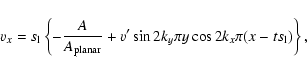 |
(4) |
We performed a number of simulations with different fuel
densities. The fuel was assumed to consist of pure carbon. For
convenience of the reader, a compilation of the setup values is
given in Table 1. The laminar burning velocities ![]() are
determined according to the formula given by Timmes & Woosley (1992);
marked "TW'' in the table.
are
determined according to the formula given by Timmes & Woosley (1992);
marked "TW'' in the table.
![\begin{figure}
\par\includegraphics[width=8.5cm,clip]{0778fig3.eps}
\end{figure}](/articles/aa/full/2004/27/aa0778/img67.gif) |
Figure 3:
a) Flame propagation into quiescent fuel at a density of 5 |
| Open with DEXTER | |
Before we present the results of our numerical study we discuss what we actually are looking for in the simulations. That is, we somehow have to define how to discriminate between stable flame propagation and a breakdown of the stabilization. Why is this a question of definition? From the conjecture of active turbulent combustion it may appear that a breakdown of the stabilization must be obvious from a rapid and unlimited growth of the flame propagation velocity. However, this cannot be expected to occur in a numerical simulation where the growth of the flame surface due to ATC would be limited by discretization and resolution. Hence, the maximum effect that can be anticipated is a rapid increase in flame surface and burning velocity and a saturation at some higher value. A second possibility is that with increasing strength the vortical flow starts to dominate the flame evolution.
On the other hand, how can we guarantee flame stabilization? Owing to the high computational costs it will not be possible to follow the flame propagation for an arbitrarily long time. However, in case of stabilization we can actually make use of the knowledge of the flame pattern that is to be expected in case of stability in our specific simulation setup. From the preceding studies of flame propagation into quiescent fuel (Röpke et al. 2003,2004) it is known that the flame finally stabilizes in a single domain-filling cusp-like structure for our setup. This structure may be superimposed by a smaller-scale cellular pattern in sufficiently resolved simulations. A similar result can be anticipated for interaction with weak imprinted vortices.
Thus we may expect two extremal behaviors of the flame. In one case the flame stabilizes and the incoming perturbation fails to break up the cellular pattern. The cells of the stabilized small wavelength pattern caused by the initial perturbation of the flame front will then merge forming the single domain-filling cusp which then propagates stably. Alternatively, if the intensity of the incoming vortices is high enough to destroy the stabilization, no single domain-filling cusp will finally emerge. In this second case the flame should rather show a transient pattern.
| |
Figure 4:
Flame interaction with a vortical fuel field at
a density of 5 |
| Open with DEXTER | |
![\begin{figure}
\par\includegraphics[width=17.1cm,clip]{0778fig5.eps}
\end{figure}](/articles/aa/full/2004/27/aa0778/img70.gif) |
Figure 5:
Flame evolution for a fuel density of 5 |
| Open with DEXTER | |
As an example, we consider the case of a fuel density amounting to 5 ![]()
![]() (cf. Table 1). Figure 3 gives an overview over
the flame evolution in interaction with vortical fuel flows of
different strengths. The values
(cf. Table 1). Figure 3 gives an overview over
the flame evolution in interaction with vortical fuel flows of
different strengths. The values
![]() ,
,
![]() ,
and
,
and
![]() indicate the amplitudes of velocity fluctuations
imposed at the right boundary of the domain. Note, however, that they
do not necessarily represent the values experienced by the flame front
for reasons given in Sect. 3.1.
indicate the amplitudes of velocity fluctuations
imposed at the right boundary of the domain. Note, however, that they
do not necessarily represent the values experienced by the flame front
for reasons given in Sect. 3.1.
Figure 3a provides the comparison with flame propagation into quiescent fuel for the chosen setup. In this simulation v'was set to zero. It resembles the features of the simulations presented by Röpke et al. (2003,2004). Due to the LD instability, the initial perturbation grows and the flame shape evolves into a cellular pattern in the nonlinear regime. The subsequent contours show the "merging'' of the short-wavelength cells imprinted by the initial condition resulting in the formation of larger cells. This behavior was observed in a simulation of the long-term flame evolution in quiescent fuel (Röpke et al. 2004). There a cusp-like structure that was centered in the domain finally emerged as the steady state structure. The tendency to form a domain-filling cell is also apparent in Fig. 3a. However, following the evolution until the steady-state is reached is very expensive and shall not be tried here. This is certainly a drawback in the current study, but it was chosen as a compromise in order to be able to explore a larger parameter space with given computational resources.
Contrary to the flame evolution in Fig. 3a, the case of
![]() (Fig. 3d) clearly shows the disruption of the initial
cellular pattern by interaction of the flame with vortices. Also, the
formation of a single domain-filling cell is suppressed by the
interaction. The overall flame shape evolution in this case can be interpreted as
an adaptation to the imprinted vortical flow structure.
This is emphasized by Fig. 5. It provides a more
detailed visualization of the interaction between the flame shape and the vortical flow, which is
characterized by the color-coded logarithm of the absolute value of the
vorticity
(Fig. 3d) clearly shows the disruption of the initial
cellular pattern by interaction of the flame with vortices. Also, the
formation of a single domain-filling cell is suppressed by the
interaction. The overall flame shape evolution in this case can be interpreted as
an adaptation to the imprinted vortical flow structure.
This is emphasized by Fig. 5. It provides a more
detailed visualization of the interaction between the flame shape and the vortical flow, which is
characterized by the color-coded logarithm of the absolute value of the
vorticity ![]() of the flow field,
of the flow field,
The transition in the flame evolution between the extreme cases
depicted in Figs. 3a and 3d does,
however, not proceed abruptly, but rather in a smooth
transition. Figures 3b,c present two examples of
intermediate behaviors at
![]() and
and
![]() ,
the first
of which is again illustrated by snapshots in Fig. 6.
In this case, still a tendency to form a long-wavelength cellular
structure is visible. Here the mechanism of the advection of
small perturbations toward the cusp (Zel'dovich et al. 1980; Röpke et al. 2003,2004) dominates over the effects of the vortical flow on the flame shape.
,
the first
of which is again illustrated by snapshots in Fig. 6.
In this case, still a tendency to form a long-wavelength cellular
structure is visible. Here the mechanism of the advection of
small perturbations toward the cusp (Zel'dovich et al. 1980; Röpke et al. 2003,2004) dominates over the effects of the vortical flow on the flame shape.
![\begin{figure}
\par\includegraphics[width=17.1cm,clip]{0778fig6.eps}
\end{figure}](/articles/aa/full/2004/27/aa0778/img72.gif) |
Figure 6:
Flame evolution for a fuel density of 5 |
| Open with DEXTER | |
Simulations similar to the aforementioned were also performed in some cases with higher resolution of the numerical grid in order to test whether or not insufficient resolution prevents small scale flame structures from developing. However, no significant difference to the flame evolution depicted in Figs. 3a-d could be noticed. An example with double resolution is given in Fig. 4. Note that here the intention is not to provide a resolution study in the strict sense. The development of the particular realization of the cellular pattern as a transient phenomenon is determined by small perturbations (including numerical noise) which cannot be reproduced in different setups. However, the important point is that the flame in both resolutions finally adapts its shape to the vortices in the incoming fuel and no features develop below the scale of these vortices, which could have been overlooked in lower resolution. This agrees with Helenbrook & Law (1999), who found in their simulations of chemical flames that the wavelength of perturbations that develop in the interaction with a vortical flow is determined by the scale of the vortices and not by a critical wavelength (introduced by a curvature-dependent burning speed of the flame front according to Markstein 1951).
In order to quantify the flame evolution as qualitatively described in the preceding section, we conducted a parameter study. It aimed at the determination of flame behavior as a function of the strength of the vortices in the incoming flow and in dependence on the fuel density.
As discussed by Röpke et al. (2004), the simulation of flame
stabilization at around 1.0 ![]()
![]() requires unaffordable high numerical resolutions and furthermore our thin flame approximation is certainly not a
realistic description of thermonuclear burning in SNe Ia at these low
densities. On the other hand, it can be observed, that at higher fuel densities (around
requires unaffordable high numerical resolutions and furthermore our thin flame approximation is certainly not a
realistic description of thermonuclear burning in SNe Ia at these low
densities. On the other hand, it can be observed, that at higher fuel densities (around
![]() )
the sensitivity of the initial flame to small-wavelength perturbations increases. This causes difficulties in producing a stable flame configuration prior to the
incoming vortices encountering the flame front. However, in
connection with a possible DDT we are mainly interested in the late
stages of the SN Ia explosions (see Sect. 1). Therefore
we restricted the study to four fuel densities:
)
the sensitivity of the initial flame to small-wavelength perturbations increases. This causes difficulties in producing a stable flame configuration prior to the
incoming vortices encountering the flame front. However, in
connection with a possible DDT we are mainly interested in the late
stages of the SN Ia explosions (see Sect. 1). Therefore
we restricted the study to four fuel densities:
![]()
![]()
![]() ,
,
![]()
![]()
![]() ,
,
![]()
![]()
![]() ,
and
,
and
![]()
![]()
![]() (cf. Table 1).
(cf. Table 1).
Plots similar to Fig. 3 corresponding to simulations with
different fuel densities are given by Röpke (2003).
The flame evolution in these simulations can be summarized as follows:
at lower fuel densities the effect of the incoming vortices on the
flame structure is generally more drastic. For
![]()
![]()
![]() the tendency of the formation of the domain-filling structure is still visible in the case of
propagation into quiescent fuel. This is not the case for
the tendency of the formation of the domain-filling structure is still visible in the case of
propagation into quiescent fuel. This is not the case for
![]()
![]()
![]() for reasons discussed by Röpke et al. (2004). However, with increasing strengths of the
imprinted velocity fluctuations, the flame still gradually adapts to
the flow for both fuel densities.
At
for reasons discussed by Röpke et al. (2004). However, with increasing strengths of the
imprinted velocity fluctuations, the flame still gradually adapts to
the flow for both fuel densities.
At
![]()
![]()
![]() the flame evolution
is similar to that at
the flame evolution
is similar to that at
![]()
![]()
![]() .
Only in case of
propagation into quiescent fuel an initial
destabilization with respect to small wavelength perturbations
(cf. Röpke et al. 2004) alters the evolution for a transition
period, before the flame finally stabilizes in a domain-filling single-cell
structure.
.
Only in case of
propagation into quiescent fuel an initial
destabilization with respect to small wavelength perturbations
(cf. Röpke et al. 2004) alters the evolution for a transition
period, before the flame finally stabilizes in a domain-filling single-cell
structure.
In a quantitative evaluation of our parameter study regarding the flame evolution for different fuel densities we will now address (i) the dependency of the effective flame propagation velocity on the strength of the imprinted velocity fluctuations and (ii) the amplification of the velocity fluctuation by the flame front.
For the exemplary case of ![]()
![]()
![]() we discuss the measurement of the necessary quantities in our simulations.
we discuss the measurement of the necessary quantities in our simulations.
The effective propagation velocity
![]() of the flame is determined via the
flame surface:
of the flame is determined via the
flame surface:
The standard deviation of the velocity field is obtained separately in
the fuel upstream of the front and in the ashes downstream of it in
order to determine the amplification of the velocity fluctuations
across the flame front. In Fig. 8 the quantities are plotted
against time for our exemplary case. As mentioned above, the strength of the
vortices produced at the inflow boundary is not a reliable measure of
what the flame actually experiences, since the velocity fluctuations
get damped quickly when propagating toward the flame and bending of
the flame front may lead to different velocity fluctuations at
different locations on the flame. Moreover, the dependence of the damping
on the fuel density hampers the comparability of simulations with this
parameter varying. Therefore we determine the standard deviations
of the velocity fields,
![]() and
and
![]() ,
within a certain belt
around the flame front. This belt was scaled in a way that the time for flame crossing over its width remained the same for all fuel densities.
,
within a certain belt
around the flame front. This belt was scaled in a way that the time for flame crossing over its width remained the same for all fuel densities.
All quantities measured in our simulations
fluctuate considerably with time. Hence we averaged them over a
time ranging from 480
![]() to 720
to 720
![]() (
(
![]() denotes the crossing time of the corresponding laminar flame over one grid cell).
denotes the crossing time of the corresponding laminar flame over one grid cell).
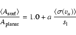
In Fig. 9 the temporal mean value of flame surface
area
![]() (normalized to the surface area of the corresponding planar flame
front
(normalized to the surface area of the corresponding planar flame
front
![]() )
is plotted against the temporal mean of standard deviation of
the velocity in the fuel region (normalized to the laminar burning
velocity of the flame).
The increase of the flame speed with stronger incoming velocity
fluctuations is evident here. However, there is
quite a large scatter in the data. This has two reasons. First, we
certainly did not follow the flame evolution long enough to
undoubtly reach the steady state of the flame shape - which should
ideally be the clearly distinct single domain-filling cusp-like
structure in case of weak incoming vortices. To follow the flame
propagation up to this stage would be much too expensive for
a parameter study. Second, some peculiar features of the flame shape may
develop as a result of small perturbations (e.g. due to numerical
noise). In particular, this may cause substantial deviations if it affects the
long-wavelength structure of the flame and is primarily responsible for the
scatter of the results in case of strong incoming velocity fluctuations. This scatter could very likely be cured by taking the mean over longer time intervals.
)
is plotted against the temporal mean of standard deviation of
the velocity in the fuel region (normalized to the laminar burning
velocity of the flame).
The increase of the flame speed with stronger incoming velocity
fluctuations is evident here. However, there is
quite a large scatter in the data. This has two reasons. First, we
certainly did not follow the flame evolution long enough to
undoubtly reach the steady state of the flame shape - which should
ideally be the clearly distinct single domain-filling cusp-like
structure in case of weak incoming vortices. To follow the flame
propagation up to this stage would be much too expensive for
a parameter study. Second, some peculiar features of the flame shape may
develop as a result of small perturbations (e.g. due to numerical
noise). In particular, this may cause substantial deviations if it affects the
long-wavelength structure of the flame and is primarily responsible for the
scatter of the results in case of strong incoming velocity fluctuations. This scatter could very likely be cured by taking the mean over longer time intervals.
![\begin{figure}
\par\includegraphics[width=7.1cm,clip]{0778fig7.eps}
\end{figure}](/articles/aa/full/2004/27/aa0778/img84.gif) |
Figure 7:
Flame surface area as function of time (normalized to the crossing time of the
laminar flame over one grid cell
|
| Open with DEXTER | |
![\begin{figure}
\par\includegraphics[width=13.45cm,clip]{0778fig8.eps}
\end{figure}](/articles/aa/full/2004/27/aa0778/img85.gif) |
Figure 8:
a), b) Standard deviation of the velocity field ahead
of the front as function of time, and c), d) ratio of the standard
deviations of the velocity fields beyond and ahead of the flame as function
time. The left and right columns of plots correspond to
|
| Open with DEXTER | |
Damköhler (1940) proposed a linear dependence of the
effective flame propagation velocity on the turbulence intensity
for turbulent combustion in what
is today called the flamelet regime (Peters 1986). Our results are consistent
with a linear growth law.
Corresponding fits to the data are included in
Fig. 9 and values for the parameter a according to the fitting formula
In order to estimate the amplification of the velocity fluctuations across the flame for different densities, we compared the strength of velocity fluctuations downstream of the flame with the strength of the imprinted vortices in the fuel. As already shown for the case of flame propagation into quiescent fuel (Röpke et al. 2004), the flame produces vorticity in the ashes. Here, the question is addressed whether vorticity present in the fuel will be amplified in the flame.
The result of the study for a variety of fuel densities is plotted in Fig. 10. In this plot, trends show up much more clearly than in Fig. 9. However, some scatter is still present in the data. As can be seen from snapshots of the evolution of the flame front (an example is depicted in Fig. 5c), the merging of cusps can eventually produce transient "bursts'' in the vorticity downstream of the flame. This is particularly prominent in case of changes in the long-wavelength flame structure, but not necessarily connected to it. From Fig. 8d, where this "burst'' in velocity fluctuation appears as a spike in the profile, it can be concluded that the duration of those events is very short. Hence their contribution to the temporal mean is small (whereas the long-wavelength flame structure and thus the flame surface change slowly). Consequently, the scatter in plot 10 is much smaller than in plot 9.
The data plotted in Fig. 10 can be fit rather well by a linear
relation between the ratio
![]() and the incoming turbulence
intensity, i.e.
and the incoming turbulence
intensity, i.e.
The above interpretation of this result requires some
caution, since the cellular stabilization of the flame has been shown
to be weaker with lower fuel density. However, this
seems to be a numerical rather than a physical effect, since the cusps
become more stable with higher resolution. Thus, at the given
resolution of our parameter study, the flame evolution shows peculiar
behavior at a fuel density of 1.25 ![]()
![]() and below. Here, cusps may loose stability distorting the flame shape, which then responds with accelerated propagation of the perturbed part for a short period, after that the flame stabilizes
again. The interaction with the vortical flow outweighs this effect in
our simulations, but the simulation at these
density may be less reliable. However, we do
not observe such a flame evolution at the higher fuel densities included
in this parameter study. Thus, the dependency on the fuel density is likely
to be (at least partially) of physical origin.
and below. Here, cusps may loose stability distorting the flame shape, which then responds with accelerated propagation of the perturbed part for a short period, after that the flame stabilizes
again. The interaction with the vortical flow outweighs this effect in
our simulations, but the simulation at these
density may be less reliable. However, we do
not observe such a flame evolution at the higher fuel densities included
in this parameter study. Thus, the dependency on the fuel density is likely
to be (at least partially) of physical origin.
![\begin{figure}
\par\includegraphics[width=8.15cm,clip]{0778fig9.eps}
\end{figure}](/articles/aa/full/2004/27/aa0778/img91.gif) |
Figure 9: Dependence of the flame surface area on the strength of the imprinted velocity fluctuations. |
| Open with DEXTER | |
![\begin{figure}
\par\includegraphics[width=8.1cm,clip]{0778fig10.eps}
\end{figure}](/articles/aa/full/2004/27/aa0778/img92.gif) |
Figure 10: Relation between velocity fluctuations upstream and downstream of the flame front. |
| Open with DEXTER | |
![\begin{figure}
\par\includegraphics[width=8.2cm,clip]{0778fig11.eps}
\end{figure}](/articles/aa/full/2004/27/aa0778/img93.gif) |
Figure 11:
Ratio of the velocities upstream and downstream of the flame
front as a function of the density contrast |
| Open with DEXTER | |
In the presented simulations we performed the first attempt to investigate the interaction of cellular flames with turbulent velocity fluctuations in the context of SN Ia explosions. The results can be summarized as follows:
Table 2: Fit parameters according to fitting formulas (7) and (8) with corresponding asymptotic standard errors.
Interaction with the incoming vortices leads to a superposition of this fundamental structure with a cellular pattern of shorter wavelength. Similar to the simulations presented by Röpke et al. (2003), where a cellular superposition of the basic flame structure was observed in case of wide computational domains, this does not lead to a destabilization of the domain-filling cell. In accord with theoretical predictions (Zel'dovich et al. 1980) the small superimposed perturbations are advected toward the cusp where they disappear. The flow field accounting for this effect was studied by Röpke et al. (2004).
Although the increase in effective flame propagation resulting from
the cellular regime is negligible compared to the increase in
flame speed at larger scales where the flame is affected by the
turbulent cascade, it may be significant in the early stages of the
explosion. In the current large-scale models (e.g., Reinecke et al. 2002), the flame is assumed to propagate with its laminar flame velocity before the rising Rayleigh-Taylor bubbles
establish the turbulent cascade. This may cause a problem with the
nucleosynthetic yields from the SN Ia explosion (Reinecke 2001). Since the laminar
flame speed is very low, the WD expands slowly in
the beginning of the explosion and thus the combustion products remain
at rather high densities for a considerable time. This effect causes
a neutronization of the material by electron capture and an
overproduction of neutron-rich heavy nuclei
(Nomoto & Kondo 1991; Brachwitz et al. 2000), eventually even leading to a collapse
of the star. Taking into account the velocity increase resulting from
the cellular regime, this problem could be extenuated. As has been
shown in this study, this may be in
particular the case if strong velocity fluctuations left over from
the pre-ignition convection interact with the flame. However, the
strength of turbulence resulting from pre-ignition effects is not
well-determined yet. Höflich & Stein (2002) claim values as high as
![]()
![]() .
The impact of the cellular
burning regime on the nucleosynthesis yields of the SN Ia explosion
models will be investigated in a forthcoming study.
.
The impact of the cellular
burning regime on the nucleosynthesis yields of the SN Ia explosion
models will be investigated in a forthcoming study.
Even though we can probably not completely rule out the possibility of active turbulent combustion, we found no convincing hint for such an effect in our numerical investigations. Our simulations indicate that effects resulting from the cellular regime of flame propagation are unlikely to trigger a presumed deflagration-to-detonation transition. Hence, the search for active turbulent combustion and deflagration-to-detonation transition should focus on the distributed burning regime.
Acknowledgements
This work was supported in part by the European Research Training Network "The Physics of Type Ia Supernova Explosions'' under contract HPRN-CT-2002-00303 and by the DFG Priority Research Program "Analysis and Numerics for Conservation Laws'' under contract HI 534/3. A pleasant atmosphere to prepare this publication was provided at the workshop "Thermonuclear Supernovae and Cosmology'' at the ECT*, Trento, Italy. We would like to thank M. Reinecke, S. Blinnikov, and W. Schmidt for stimulating discussions. The numerical simulations were performed on an IBM Regatta system at the computer center of the Max Planck Society in Garching.