A&A 421, 681-691 (2004)
DOI: 10.1051/0004-6361:20040228
R. T. Edwards1 - B. W. Stappers1,2
1 - Astronomical Institute "Anton Pannekoek'',
University of Amsterdam,
Kruislaan 403, 1098 SJ Amsterdam, The Netherlands
2 -
Stichting ASTRON, Postbus 2, 7990 AA Dwingeloo, The Netherlands
Received 9 February 2004 / Accepted 26 March 2004
Abstract
We report on an analysis of the polarization of single
pulses of PSR B0329+54 at 328 MHz. We find that the distribution of
polarization orientations in the central component diverges strongly
from the standard picture of orthogonal polarization modes (OPMs),
making a remarkable partial annulus on the Poincaré sphere. A
second, tightly clustered region of density appears in the opposite
hemisphere, at a point antipodal to the centre of the annulus. We
argue that this can be understood in terms of birefringent alterations
in the relative phase of two elliptically polarized propagation modes
in the pulsar magnetosphere (i.e. generalised Faraday rotation). The
ellipticity of the modes implies a significant charge density in the
plasma, while the presence of both senses of circular polarization,
and the fact that only one mode shows the effect, supports the view
that refracted ordinary-mode rays are involved in the production of
the annulus. At other pulse longitudes the polarization (including
the circular component) is broadly consistent with an origin in
elliptical OPMs, shown here quantitatively for the first time, however
considerable non-orthogonal contributions serve to broaden the
orientation distribution in an isotropic manner.
Key words: plasmas - polarization - stars: pulsars: individual: PSR B0329+54 - waves
Whenever sufficient sensitivity is available, radio pulsar emissions
are seen to be rich in phenomenology. Their polarization is no
exception to this rule. The dependence of linear polarization position
angle on pulse longitude (i.e. rotational phase) can, for some
pulsars, be explained as arising in the vicinity of the magnetic
pole, polarized linearly at the position angle of the sky projection
of magnetic field lines (Radhakrishnan & Cooke 1969). For other pulsars this is not
the case, and for some of these the distribution of position angles
(PAs) in individual pulses has been shown to be bimodal about two
values separated by 90
![]() - so-called orthogonal polarization
modes (OPMs; e.g. Cordes et al. 1978; Manchester et al. 1975; Stinebring et al. 1984a,b; Backer et al. 1976; Backer & Rankin 1980).
Many pulsars also show
- so-called orthogonal polarization
modes (OPMs; e.g. Cordes et al. 1978; Manchester et al. 1975; Stinebring et al. 1984a,b; Backer et al. 1976; Backer & Rankin 1980).
Many pulsars also show
![]() "jumps'' in their position angle
profiles, a fact that received explanation in the discovery of OPMs
through a longitude dependence of the relative intensities of the
modes, which themselves tend to have position angle swings
consistent with the magnetic pole model of Radhakrishnan & Cooke (1969). These
studies of OPMs also found evidence for deviations from orthogonality
in the fact that PA distributions were broader than expected and/or
their peaks were not separated by
"jumps'' in their position angle
profiles, a fact that received explanation in the discovery of OPMs
through a longitude dependence of the relative intensities of the
modes, which themselves tend to have position angle swings
consistent with the magnetic pole model of Radhakrishnan & Cooke (1969). These
studies of OPMs also found evidence for deviations from orthogonality
in the fact that PA distributions were broader than expected and/or
their peaks were not separated by
![]() .
.
Attempts have been made to explain these deviations from orthogonality by means of superposition of two modes that are not orthogonal due to origins on different field lines and subsequent birefringent refraction (e.g. McKinnon 2003a; Stinebring et al. 1984a), by means of the superposition of a range of modal orientations arising from a distribution of field lines that are visible due to their finite beam width (Gil & Lyne 1995), or due to the presence of two instantaneously orthogonal modes, the orientation of which varies with time due to coherent wave coupling effects (e.g. Lyubarskii & Petrova 1999; Cheng & Ruderman 1979). Of these, only the first and third scenarios have been quantitatively tested. McKinnon (2003a) showed that the distribution of PAs, and the shape of the average PA curve of PSR B2016+28 are consistent with the superposition of two non-orthogonal modes. On the other hand, Petrova (2003) showed that the PA and circular polarization of the average pulse profiles of PSR B0355+54 and PSR B0628-28 are consistent with the predictions of Lyubarskii & Petrova (1999) for alterations in the polarization due to coherent effects. However, neither work examines whether the data are also consistent with other models, and indeed the statistics considered in each case are not well suited to distinguishing between models.
The question of the origin of circular polarization in pulsars is also not addressed by the magnetic pole model, in which the polarization is expected to be linear due to the high magnetic field strength. The fact that orthogonal linear polarization states have been found to be associated with opposite signs of circular polarization leads naturally to the suggestion that the modes are in fact elliptically polarized orthogonal modes (Cordes et al. 1978), although to our knowledge, to date no observational tests of the expected proportionality between linear and circular polarization under this hypothesis have been made. In explaining the origin of elliptical OPMs, most authors point to the so-called polarization-limiting region (PLR), where birefringent propagation effects no longer significantly alter the relative phase of the modes, as the determinant of the observed polarization (Cheng & Ruderman 1979). It has been proposed that either the propagation modes themselves are elliptical at this point, requiring a net charge density in the plasma (von Hoensbroech et al. 1998; Cheng & Ruderman 1979; Allen & Melrose 1982), or that weak birefringence in the vicinity of the PLR causes initially linearly polarized rays to suffer changes in their polarization if their position angle deviates from that of the local linear modes, for example due to rotational aberration or refraction (Lyubarskii & Petrova 1999; Petrova 2001; Cheng & Ruderman 1979; Petrova & Lyubarskii 2000; Petrova 2003).
In this work we make a detailed study of the polarization of single pulses from PSR B0329+54, employing new techniques in the hope of placing greater constraints on the nature and origin of ellipticity and non-orthogonality of pulsar polarization.
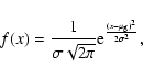
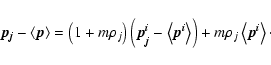
Since the focus of this study is the inconsistency of observations with a simple model of superposed OPMs, it is pertinent to begin with a clear picture of the features expected under such a model, before discussing ways in which the observations may deviate from it. The distribution of Stokes parameters expected under the incoherent superposition of two elliptical OPMs, and techniques for reconstruction of the modal intensities have been considered in detail by McKinnon & Stinebring (2000).We briefly re-iterate in a more compact vector form before considering the fluctuation statistics.
The modes are taken to be completely polarized, with fixed position
angles and degrees of circular polarization at a given pulse
longitude. This means that the vector
![]() for a given mode i always has the same orientation, regardless of its
length (i.e. the intensity of the mode). The condition of
orthogonality of the electric field vectors requires that the
polarization states be antiparallel in the Poincaré sphere
(
for a given mode i always has the same orientation, regardless of its
length (i.e. the intensity of the mode). The condition of
orthogonality of the electric field vectors requires that the
polarization states be antiparallel in the Poincaré sphere
(![]() -space). Since the Stokes 4-vector of the incoherent sum of
two polarization states is simply the sum of their respective Stokes
vectors, all resultant states must lie on the line defined by the
modal orientation. The observed Stokes parameters at any instant
can be written as:
-space). Since the Stokes 4-vector of the incoherent sum of
two polarization states is simply the sum of their respective Stokes
vectors, all resultant states must lie on the line defined by the
modal orientation. The observed Stokes parameters at any instant
can be written as:
The procedure of
"mode separation'' (determination of modal intensities) follows
directly as:
By measuring appropriate statistics of the Stokes vectors, information
is available on the fluctuation statistics of the OPMs. Characterising
the latter by the modal variances
![]() and
and
![]() and
their covariance
and
their covariance
![]() ,
one observes that
,
one observes that
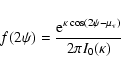
The defining feature of elliptical OPMs is the predicted constant
orientation of ![]() ,
regardless of pulse-to-pulse fluctuations in
I and
,
regardless of pulse-to-pulse fluctuations in
I and ![]() .
This fact is put to good use in the display of
histograms of the position angle of linear polarization,
.
This fact is put to good use in the display of
histograms of the position angle of linear polarization,
![]() ,
which at a given longitude can take
one of two allowed values offset by
,
which at a given longitude can take
one of two allowed values offset by
![]() .
In the presence of
instrumental noise these broaden to give the characteristic bimodal
distribution of OPM. The position angle distribution gives information
on the orthogonality of the linear component of the polarization, but
the question must also be asked whether the circular component is as
expected under elliptical OPM. Attempts to answer this question
have been hampered in the past due to the use of inappropriate
statistics. McKinnon (2002) notes that the picture of elliptical OPM is
consistent with observations showing distributions of Stokes V/Ithat are broad and centred near zero (Stinebring et al. 1984a; Backer & Rankin 1980) (or
equivalently, we note, that
.
In the presence of
instrumental noise these broaden to give the characteristic bimodal
distribution of OPM. The position angle distribution gives information
on the orthogonality of the linear component of the polarization, but
the question must also be asked whether the circular component is as
expected under elliptical OPM. Attempts to answer this question
have been hampered in the past due to the use of inappropriate
statistics. McKinnon (2002) notes that the picture of elliptical OPM is
consistent with observations showing distributions of Stokes V/Ithat are broad and centred near zero (Stinebring et al. 1984a; Backer & Rankin 1980) (or
equivalently, we note, that
![]() tends to greatly exceed
tends to greatly exceed
![]() ;
Karastergiou et al. 2003). However, such a distribution
could not be considered a particularly distinctive feature of OPM and
could easily be produced even by a mechanism for the production of
circular polarization that is independent of the linear OPM
phenomenon. A much more stringent test is to check that the observed
V is, along with Q and U, consistent with a constant orientation
of
;
Karastergiou et al. 2003). However, such a distribution
could not be considered a particularly distinctive feature of OPM and
could easily be produced even by a mechanism for the production of
circular polarization that is independent of the linear OPM
phenomenon. A much more stringent test is to check that the observed
V is, along with Q and U, consistent with a constant orientation
of ![]() .
The natural complement to the position angle in this
regard is the ellipticity angle,
.
The natural complement to the position angle in this
regard is the ellipticity angle,
![]() : together they completely specify the orientation
of
: together they completely specify the orientation
of ![]() via the spherical coordinate angles
via the spherical coordinate angles
![]() .
The
distributions in both parameters should be bimodal under OPM (unless
one mode always dominates), unlike the distribution of V/I,
which may be unimodal.
.
The
distributions in both parameters should be bimodal under OPM (unless
one mode always dominates), unlike the distribution of V/I,
which may be unimodal.
While a measurement of the joint probability density function,
![]() ,
contains sufficient information to detect the presence
of elliptical OPM, this choice of parameterisation is not ideal. This
is because a given solid angle element on the Poincaré sphere
subtends an area in
,
contains sufficient information to detect the presence
of elliptical OPM, this choice of parameterisation is not ideal. This
is because a given solid angle element on the Poincaré sphere
subtends an area in ![]() -space that itself depends on
-space that itself depends on ![]() .
Specifically,
.
Specifically,
| (8) |
A solution to this problem is to measure
![]() ,
which
satisfies the equal-area condition
,
which
satisfies the equal-area condition
| (9) |
To examine the distribution of polarization orientations at a single
pulse longitude, it is desirable to have minimum (zero) distortion at
both of the orientations associated with the OPMs. A cylindrical
equal-area projection with its equator containing the OPM orientations
would suffice, however the nature of deviations from OPM in PSR B0329+54
we describe below motivates the use of a projection where the distortion
is axisymmetric about the modal orientation. The only such projection
to also have the equal area property is Lambert's azimuthal equal
area projection, f(x,y) where
| x | = | (10) | |
| y | = | (11) | |
| = | (12) |
From the fact that OPMs contribute to the observed values of ![]() only along a single vector, it follows that a simple and direct means
of detecting non-orthogonal emission is to check the statistics of the
components of
only along a single vector, it follows that a simple and direct means
of detecting non-orthogonal emission is to check the statistics of the
components of ![]() perpendicular to
perpendicular to ![]() .
In order to do
this, it is necessary to define a new orthogonal basis for
.
In order to do
this, it is necessary to define a new orthogonal basis for ![]() ,
which has
,
which has ![]() as one of the basis vectors. The question then
arises of what to use for a working value of
as one of the basis vectors. The question then
arises of what to use for a working value of ![]() ,
since when
the orthogonality of all states is in question, the mean
polarization vector may not be parallel to
,
since when
the orthogonality of all states is in question, the mean
polarization vector may not be parallel to ![]() .
Under the
assumption that the majority of the fluctuations in
.
Under the
assumption that the majority of the fluctuations in ![]() are
directed along
are
directed along ![]() ,
a sensible choice for this vector is the
direction of greatest variance in
,
a sensible choice for this vector is the
direction of greatest variance in ![]() ,
which is also the
least-squares estimate of the direction of fluctuations. The method
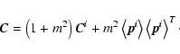
of Principal Components Analysis (PCA; e.g. Jollife 1986) is
suggested as a means of finding this vector. PCA is based on the fact
that the set of eigenvectors of the covariance matrix of a
multivariate statistic represent an orthogonal basis in which the
variations in the different axes have zero covariance
,
which is also the
least-squares estimate of the direction of fluctuations. The method
of Principal Components Analysis (PCA; e.g. Jollife 1986) is
suggested as a means of finding this vector. PCA is based on the fact
that the set of eigenvectors of the covariance matrix of a
multivariate statistic represent an orthogonal basis in which the
variations in the different axes have zero covariance![]() . That is, given the covariance matrix
. That is, given the covariance matrix
| (14) |
It is easily shown that the covariance matrix is diagonal if the
vectors are expressed using the eigenvectors as a basis. That is:
| |
= | (15) | |
| = |  |
(16) |
Clearly, the eigenvalues are equal to the variances in the components
aligned with the corresponding vectors. The eigenvector with the
greatest eigenvalue corresponds to our choice of ![]() ,
while
the other vectors and their associated eigenvalues present a
convenient basis for detection and characterisation of non-orthogonal
radiation. In theory there may be fewer than three distinct
eigenvalues indicating axisymmetry (two eigenvalues) or isotropy (one
eigenvalue) in the directional variance, although the presence of
measurement noise makes this have zero probability in practice.
However, measurement noise also introduces bias to the covariance
matrix that should be corrected by subtraction of the covariance of
the noise, estimated from off-pulse longitudes and including also
the contribution of the pulsar to the system temperature if significant.
Where the intrinsic
covariance is of a similar magnitude to the uncertainty in the
off-pulse covariance, this may result in negative eigenvalues, which
presents a problem if
,
while
the other vectors and their associated eigenvalues present a
convenient basis for detection and characterisation of non-orthogonal
radiation. In theory there may be fewer than three distinct
eigenvalues indicating axisymmetry (two eigenvalues) or isotropy (one
eigenvalue) in the directional variance, although the presence of
measurement noise makes this have zero probability in practice.
However, measurement noise also introduces bias to the covariance
matrix that should be corrected by subtraction of the covariance of
the noise, estimated from off-pulse longitudes and including also
the contribution of the pulsar to the system temperature if significant.
Where the intrinsic
covariance is of a similar magnitude to the uncertainty in the
off-pulse covariance, this may result in negative eigenvalues, which
presents a problem if
![]() is to be used as a measure of
the scale of intensity fluctuations, and it must be accepted that
estimates will be unavailable in some longitude bins. This problem is
also familiar from, for example, bias-corrected estimates of the
linearly polarized intensity,
is to be used as a measure of
the scale of intensity fluctuations, and it must be accepted that
estimates will be unavailable in some longitude bins. This problem is
also familiar from, for example, bias-corrected estimates of the
linearly polarized intensity,
![]() .
.
Having measured the variance of fluctuations in components parallel to
and perpendicular to the modal orientation, it is useful to define a
measure of the degree of deviation from purely linear
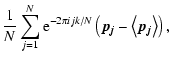
fluctuations. After Cloude & Pottier (1995), we define the polarization entropy
as:
The methods of the previous section work from the covariance
of the observed signal, which in practice may reflect not only the
intrinsic variations of the pulsar, but also the effects of the
interstellar medium on the propagating signal. Of principle importance
is the variable effective gain of the interstellar medium induced by
two types of propagation effect, refractive and diffractive
scintillation. For most pulsars, the time scale for variations due to
refractive scintillation is long (![]() 15 days for PSR B0329+54;
Stinebring et al. 2000), so the effects can be neglected over short
observations. Time scales for diffractive scintillation, on the other
hand, are much shorter. In some cases the time scale may be long
enough that one can simply limit the analysis to a segment of time
over which the flux density is constant (e.g. McKinnon 2004), but in
other cases such intervals do not last long enough to sensitively
obtain representative statistics. With a diffractive scintillation
time scale of
15 days for PSR B0329+54;
Stinebring et al. 2000), so the effects can be neglected over short
observations. Time scales for diffractive scintillation, on the other
hand, are much shorter. In some cases the time scale may be long
enough that one can simply limit the analysis to a segment of time
over which the flux density is constant (e.g. McKinnon 2004), but in
other cases such intervals do not last long enough to sensitively
obtain representative statistics. With a diffractive scintillation
time scale of ![]() 148 s at 328 MHz (Cordes 1986), this is the case
for the observations of PSR B0329+54 reported here.
148 s at 328 MHz (Cordes 1986), this is the case
for the observations of PSR B0329+54 reported here.
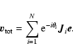
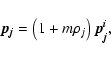
In order to separate the (co-)variance induced by scintillation from
that intrinsic to the pulsar, we employ fluctuation spectral
techniques (Edwards & Stappers 2003). We define the (longitude-resolved)
polarization spectral density tensor as the element-wise product of
the (discrete, vector) Fourier transform of
![]() with its Hermitian transpose, where
j indexes pulse number and the longitude dependence is implicit as
elsewhere in this work. That is,
with its Hermitian transpose, where
j indexes pulse number and the longitude dependence is implicit as
elsewhere in this work. That is,
The effect of scintillation on the observed signal ![]() is
a time-varying, multiplicative gain. The observed signal can be written
is
a time-varying, multiplicative gain. The observed signal can be written
![\begin{figure}
\par\includegraphics[width=11.25cm,clip]{aa0228-04f1.eps} %\end{figure}](/articles/aa/full/2004/26/aa0228-04/img80.gif) |
Figure 1:
Longitude-dependent polarization behaviour of PSR B0329+54 in
its normal profile mode at 328 MHz. Plotted are the mean total and
polarized intensity (black and red, top panel) and histograms of
position angle (middle panel, plotted twice for continuity) and
|
![\begin{figure}
\par\includegraphics[clip]{aa0228-04f2.eps}
\end{figure}](/articles/aa/full/2004/26/aa0228-04/img81.gif) |
Figure 2:
Distribution of polarization orientations in eight longitude
intervals, marked in the pulse profile at the bottom and shown in
left-to-right, top-to-bottom order. Each panel shows the distribution in
Lambert's azimuthal equal-area projection with poles set near to the
typical orientation of the mode showing the least scatter. The projection is
interrupted at the equator and plotted in two hemispheres, to give low
distortion near both poles, marked by asterisks. Lines of constant
|
We used the Westerbork Synthesis Radio Telescope with the PuMa pulsar
backend (Voûte et al. 2002) to observe PSR B0329+54 in a 10 MHz band
centred at 328 MHz. PuMa was configured as a digital filterbank,
producing samples in all four Stokes parameters over 128 frequency
channels with a sample interval of 409.6 ![]() s. We found that our
standard digitisation using 2 bits per sample per channel was
insufficient to avoid clipping the brightest pulses, and caution that
this may also have been a problem in previously published polarimetry
of this and other bright pulsars. This problem was avoided by
re-observation of the pulsar with 8 bits of digitisation. In offline
analysis the data were corrected for instrumental polarization effects
determined using the procedure described in the Appendix, followed by
removal of the frequency-dependent position angle rotation caused by
interstellar Faraday rotation, and samples were summed across all
frequency channels after correcting for delays due to interstellar
dispersion. The resultant time series was divided into segments
corresponding to the apparent pulse period to give an array of 16400
pulses in 1744 pulse longitude bins, 220 of which were used in
further analysis.
s. We found that our
standard digitisation using 2 bits per sample per channel was
insufficient to avoid clipping the brightest pulses, and caution that
this may also have been a problem in previously published polarimetry
of this and other bright pulsars. This problem was avoided by
re-observation of the pulsar with 8 bits of digitisation. In offline
analysis the data were corrected for instrumental polarization effects
determined using the procedure described in the Appendix, followed by
removal of the frequency-dependent position angle rotation caused by
interstellar Faraday rotation, and samples were summed across all
frequency channels after correcting for delays due to interstellar
dispersion. The resultant time series was divided into segments
corresponding to the apparent pulse period to give an array of 16400
pulses in 1744 pulse longitude bins, 220 of which were used in
further analysis.
This pulsar is known to exhibit at least four main modes of emission,
each with a different pulse profile (Bartel et al. 1982), two of which
are commonly seen at low frequencies. By forming pulse profiles
in sub-integrations of 100 pulses, we determined that the pulsar
underwent a mode change at pulse number ![]() 12 800. The profiles
formed by adding pulses 0-12 500 and 13 000-16 400 are consistent
with the so-called "normal'' and "abnormal'' modes reported by
previous authors.
12 800. The profiles
formed by adding pulses 0-12 500 and 13 000-16 400 are consistent
with the so-called "normal'' and "abnormal'' modes reported by
previous authors.
The histograms for the abnormal mode were qualitatively very similar
to those of the normal mode, upon which the remainder of the
discussion will focus. However, we note as an aside that the position
angle distributions appeared offset between the two profile
modes. Although the presence of non-OPM means that the magnetic pole
model of Radhakrishnan & Cooke (1969) is not strictly applicable, for the purpose of
quantifying the offset, after Gil & Lyne (1995) we attempted to fit the
model to position angles determined using local maxima in the
histograms near to a curve made by eye to approximately fit the less
distorted of the polarization modes (Fig. 1). We
found that for the abnormal mode, a fit to the fiducial position angle
parameter ![]() while using values determined from the normal mode
for other parameters performed much better than a fit where
while using values determined from the normal mode
for other parameters performed much better than a fit where ![]() was fixed and all others allowed to vary (rms deviation
was fixed and all others allowed to vary (rms deviation
![]() versus
versus
![]() ), and was comparable to the best fit with all
parameters allowed to vary (rms
), and was comparable to the best fit with all
parameters allowed to vary (rms
![]() ). We therefore conclude
that the offset is consistent with a shift in position angle of
). We therefore conclude
that the offset is consistent with a shift in position angle of ![]()
![]() ,
rather than a change in the apparent viewing geometry or a
longitude offset as might be induced by differential aberration and
retardation.
,
rather than a change in the apparent viewing geometry or a
longitude offset as might be induced by differential aberration and
retardation.
While the position angle distribution of Fig. 1 is
consistent with previously published results of lower resolution
showing quasi-orthogonal modes (Gil & Lyne 1995), the ellipticity
distribution shows features of a kind never seen before in any pulsar,
owing most likely to the fact that previous studies have used V/Iinstead of ellipticity, causing OPM-related features to be washed out
due to fluctuations in
![]() .
Most striking is the strong
right-circular polarization seen under the main central component,
which has no corresponding left-circular component of equal
ellipticity as would be expected if the circular polarization is due
to the OPM clearly seen in the position angle distribution
(Sects. 2.1 and 2.2). Also of interest
is that the trailing component (longitude
.
Most striking is the strong
right-circular polarization seen under the main central component,
which has no corresponding left-circular component of equal
ellipticity as would be expected if the circular polarization is due
to the OPM clearly seen in the position angle distribution
(Sects. 2.1 and 2.2). Also of interest
is that the trailing component (longitude ![]()
![]() )
has a
distribution that is roughly bimodal about the zero line, as expected
under elliptical OPM, while the leading component (longitude
)
has a
distribution that is roughly bimodal about the zero line, as expected
under elliptical OPM, while the leading component (longitude
![]() )
appears to have a unimodal ellipticity distribution. Also
apparent is that polarized emission is occasionally detected in the
vicinity of pulse longitudes
)
appears to have a unimodal ellipticity distribution. Also
apparent is that polarized emission is occasionally detected in the
vicinity of pulse longitudes
![]() and
and
![]() ,
corresponding to
the additional emission components detected in total intensity by
Gangadhara & Gupta (2001).
,
corresponding to
the additional emission components detected in total intensity by
Gangadhara & Gupta (2001).
Much more intriguing behaviour is made apparent when the full
two-dimensional orientation distribution is considered for particular
longitude ranges. In Fig. 2 we display these distributions
averaged over several longitude intervals, using the
projection described in Sect. 2.2. In what follows
we refer to the modes occurring in the left and right halves of each
projection as modes "1'' and "2'' respectively. Addressing the
distributions in longitude order, we see that the leading component is
consistent with purely linear OPM in mode 2, while by pulse longitude
![]() the modes have switched in dominance and become somewhat
elliptical. As the pulsar rotates, mode 2 begins to increase again
in strength, and apparently has a greater spread in its orientations
than mode 1. Over the course of the central component the distribution
associated with mode 2 deforms into an arc and eventually an almost
complete annulus, while mode 1 remains tightly distributed around
an elliptical orientation and eventually concedes dominance to mode 2.
Finally, in the trailing component the modes are of comparable
strength and distributed tightly around orthogonal elliptical
orientations. We discuss our interpretation of this remarkable
behaviour in Sect. 3.4 but first discuss the remaining
observational results.
the modes have switched in dominance and become somewhat
elliptical. As the pulsar rotates, mode 2 begins to increase again
in strength, and apparently has a greater spread in its orientations
than mode 1. Over the course of the central component the distribution
associated with mode 2 deforms into an arc and eventually an almost
complete annulus, while mode 1 remains tightly distributed around
an elliptical orientation and eventually concedes dominance to mode 2.
Finally, in the trailing component the modes are of comparable
strength and distributed tightly around orthogonal elliptical
orientations. We discuss our interpretation of this remarkable
behaviour in Sect. 3.4 but first discuss the remaining
observational results.
The results of the previous section leave no doubt that the central
component shows strong deviation from the behaviour expected under
OPM. The case of the leading and trailing components is more difficult
to assess due to the fact that the expected spread in orientations
under instrumental noise depends in a complicated way on the
distribution of ![]() .
Instead, we used the method of
eigenanalysis described in Sect. 2.3.1. In our case the
dispersed pulsar signal contributes at most about one fifth of the
total system temperature, justifying the use of a single,
longitude-independent correction to the spectral density
tensor for the off-pulse noise, under the caveat that a very small
(
.
Instead, we used the method of
eigenanalysis described in Sect. 2.3.1. In our case the
dispersed pulsar signal contributes at most about one fifth of the
total system temperature, justifying the use of a single,
longitude-independent correction to the spectral density
tensor for the off-pulse noise, under the caveat that a very small
(
![]() normalized flux units) amount of measurement
noise contaminates the variances for the central component.
The characterstic frequency corresponding to scintillation on the
diffractive time scale (148 s; Cordes 1986) is
normalized flux units) amount of measurement
noise contaminates the variances for the central component.
The characterstic frequency corresponding to scintillation on the
diffractive time scale (148 s; Cordes 1986) is ![]() 1/200 cycles
per period. To ensure the response was eliminated over its full
frequency extent, we excluded elements of the spectral density
tensor with
1/200 cycles
per period. To ensure the response was eliminated over its full
frequency extent, we excluded elements of the spectral density
tensor with
![]() when computing the covariance matrix.
Using power from
when computing the covariance matrix.
Using power from
![]() in the fluctuation
spectrum of the pulse energy, we measure a modulation index of 0.16due to scintillation, in agreement with the measurements and empirical
model of Cordes (1986), given our observing band. This value
was used to correct the overall scale of the covariance matrix. The
results of the eigenanalysis of this matrix are shown in
Fig. 3.
in the fluctuation
spectrum of the pulse energy, we measure a modulation index of 0.16due to scintillation, in agreement with the measurements and empirical
model of Cordes (1986), given our observing band. This value
was used to correct the overall scale of the covariance matrix. The
results of the eigenanalysis of this matrix are shown in
Fig. 3.
![\begin{figure}
\par {\includegraphics[width=7.5cm,clip]{0228f3.eps} }\end{figure}](/articles/aa/full/2004/26/aa0228-04/img98.gif) |
Figure 3:
Results of eigenanalysis. The top panel shows the average
intensity profile (thick solid line), the square roots of the
eigenvalues (solid, dashed, dotted thin lines, in descending order of
value), and the polarization entropy (Eq. (17); thick dotted
line). The middle panel
shows the position angle of the mean polarization vector (thick line,
plotted repeatedly at offsets of
|
Beginning with the polarization
entropy (Eq. (17)), we see that the polarization is most
disordered in the central component, as one might expect from the
distributions seen in the previous sections, but still shows
detectable entropy in all other pulse longitudes accessible to
measurement. That the divergence from pure OPM is significant is
confirmed by the fact that significant variance is detected in the
second and third eigenvalues under every component. The fact that the
second and third eigenvalues are nearly equal in all components except
the central peak indicates that, for these pulse longitudes, the
deviations from OPM show no preferred direction, and cannot be caused
by position angle distortions or a random circular component
alone. This is consistent with the analysis of PSR B1929+10 and PSR
B2020+28 at 1404 MHz performed by McKinnon (2004), who suggests the
superposition of (isotropic) randomly polarized radiation (RPR) as the
cause. On the other hand, in the central component of PSR B0329+54 all
three eigenvalues are significantly different, and indeed the analysis
of the directional distribution in the preceding section shows that
the distribution of ![]() cannot be ellipsoidal. This implies that
the deviations are themselves associated with the production of OPM,
as discussed further below.
cannot be ellipsoidal. This implies that
the deviations are themselves associated with the production of OPM,
as discussed further below.
It is also interesting to note that there is a suggestion of
correspondence between transitions in the mean modal dominance
(e.g. Fig. 1) and local minima in the polarization
entropy (Fig. 3). This appears to be the case around
pulse longitudes ![]()
![]() ,
,
![]()
![]() ,
and
,
and ![]()
![]() ,
however the correspondence is not exact, particularly in the leading
component. If the trend is in fact real and confirmed in other
pulsars, it would require that any mechanism for the production of two
OPMs predicts that under conditions leading to OPMs of similar
intensity, OPM-related fluctuations dominate more strongly over the
randomly polarized fluctuations than elsewhere in the pulse profile.
This could be the case if the modal intensities tend to be more
variable or more negatively correlated (Eq. (6)),
and/or the randomly polarized component is weaker or less
isotropic. A detailed study of a larger sample of pulsars would be
necessary to distinguish between these possibilities.
,
however the correspondence is not exact, particularly in the leading
component. If the trend is in fact real and confirmed in other
pulsars, it would require that any mechanism for the production of two
OPMs predicts that under conditions leading to OPMs of similar
intensity, OPM-related fluctuations dominate more strongly over the
randomly polarized fluctuations than elsewhere in the pulse profile.
This could be the case if the modal intensities tend to be more
variable or more negatively correlated (Eq. (6)),
and/or the randomly polarized component is weaker or less
isotropic. A detailed study of a larger sample of pulsars would be
necessary to distinguish between these possibilities.
We also note that a smooth position angle curve can be constructed
from the eigenvector corresponding to the largest eigenvalue, in
contrast to the position angle of the average polarization vector,
which shows gradual
![]() transitions rather than sharp flips as
would be needed for reconstruction of a continuous smooth curve. Also
the ellipticity angle curve of the first eigenvector avoids the
problem seen at longitude
transitions rather than sharp flips as
would be needed for reconstruction of a continuous smooth curve. Also
the ellipticity angle curve of the first eigenvector avoids the
problem seen at longitude ![]()
![]() ,
where near complete
cancelling of the linear contributions of the OPMs is not accompanied
by cancelling of the circular component, giving rise to a "spike'' in
,
where near complete
cancelling of the linear contributions of the OPMs is not accompanied
by cancelling of the circular component, giving rise to a "spike'' in
![]() where
where
![]() sweeps over the left-circular pole (indicating, incidentally,
non-orthogonal modes, or a consistent, superposed left-circularly
polarized component). These properties will likely make eigenanalysis
a useful technique for detecting polarization fluctuations driven by
OPMs and determining the longitude dependence of their polarization
orientations, even when the signal-to-noise ratio is insufficient to
detect individual pulses.
sweeps over the left-circular pole (indicating, incidentally,
non-orthogonal modes, or a consistent, superposed left-circularly
polarized component). These properties will likely make eigenanalysis
a useful technique for detecting polarization fluctuations driven by
OPMs and determining the longitude dependence of their polarization
orientations, even when the signal-to-noise ratio is insufficient to
detect individual pulses.
A possible origin for this behaviour lies in birefringent effects in
the magnetosphere. Specifically, the annular form is suggestive of a
propagation effect whereby the polarization state of incoming rays as
represented on the Poincaré sphere are rotated by a time-varying
angle about the axis defined by the central point of the annulus. Such
an effect is expected if the observed radiation passes through a
region of plasma where the natural propagation modes are different to
the ray polarization, and a net phase delay occurs between the
components of the electric field in each of the two modes due to their
different group velocities. This effect has been termed Generalised
Faraday Rotation (GFR; Kennett & Melrose 1998) and is familiar from, but not
theoretically limited to, ordinary Faraday rotation in the
interstellar medium (about Stokes V, due to the circular modes of
cold, non-relativistic magnetised plasma), and from the effect of
retardation plates (rotation of ![]() about a linear orientation
defined by the optical axis of the material). In the case of the
pulsar, the polarization of the plasma modes can be identified with
the slightly elliptical polarization states that appear antipodal on
the Poincaré sphere at the centre of the annulus and at the
typical orientation of states dominated by the other, well-behaved
mode. The incoherent superposition of radiation in the other
polarization mode, which apparently does not suffer this effect, would
cause the annulus to broaden outwards, helping to explain the spread
of the observed distribution.
about a linear orientation
defined by the optical axis of the material). In the case of the
pulsar, the polarization of the plasma modes can be identified with
the slightly elliptical polarization states that appear antipodal on
the Poincaré sphere at the centre of the annulus and at the
typical orientation of states dominated by the other, well-behaved
mode. The incoherent superposition of radiation in the other
polarization mode, which apparently does not suffer this effect, would
cause the annulus to broaden outwards, helping to explain the spread
of the observed distribution.
This kind of effect was predicted for pulsar magnetospheres by Cheng & Ruderman (1979) and given a quantitative treatment by Lyubarskii & Petrova (1999). In their formulation the change in polarization is effected in the vicinity of the polarization limiting region (PLR; Sect. 1), where the plasma density is insufficient to cause total decoherence of the modes, yet densities are still high enough to cause significant phase delays between the modes. Radiation enters this region as an incoherent mixture of the local plasma modes, but due to changes in the modal orientation along the ray path caused by the rotation of the magnetosphere, each of the incoming rays acquires components in both of the propagation modes, which propagate at different speeds and alter the polarization of the ray accordingly. This picture deviates from our observations in several ways. Firstly, Lyubarskii & Petrova (1999) assume linearly polarized propagation modes, whereas the observations indicate elliptical modes, implying plasma with a net charge density rather than a pure pair plasma. Secondly, the predicted effect is not as simple as rotation about a given axis, for the modal polarization orientation, and thus the axis of rotation, varies along the ray path. The presence of an annular shape, as expected from a near-constant polarization of the propagation modes, may therefore place some constraints on the size of the region of the magnetosphere contributing significant, variable amounts of GFR. Finally, the effect should only be capable of inducing one sense of circular polarization (Lyubarskii & Petrova 1999; Radhakrishnan & Rankin 1990), and should affect both rays equally apart from a reversal in the sense of circular polarization (Petrova 2001).
An alternative cause of the misalignment of the polarization of the propagation modes and the incoming rays, is refraction. Petrova & Lyubarskii (2000) show that, while the extraodinary mode propagates under a vacuum dispersion law, the ordinary mode can suffer from significant refraction, which, under a non-axisymmetric plasma distribution, can cause it to move out of the plane of the magnetic field line from which it originated (and obtained its initial polarization). The calculations of Petrova & Lyubarskii (2000) show that the subsequent alteration of the polarization state at the PLR can produce either sense of circular polarization, as seen in our observations. Moreover, since the extraordinary mode is immune to refraction, it should not suffer the same PLR effects, consistent with the tight, centrally peaked distributions of orientations observed here in mode 1. Should one of the modes be produced by conversion from the other, as in Petrova (2001), this would imply that refraction occurs above the conversion region. An alternative means of producing mode-dependent PLR effects is the invocation of [anti-]correlation between the efficiency of conversion and the physical conditions in the PLR (Petrova 2001), however for this to be the case the correlation must be very strong, given the complete absence of an annulus in the distribution of states apparently dominated by mode 2. That refraction-driven PLR effects only occur close to the magnetic axis (Petrova & Lyubarskii 2000) is another prediction borne out by the observation that only the central profile component shows the annular distribution. Many pulsars show strong mean circular polarization in central, so-called "core'' components (Rankin 1983), which tends to show a central sense reversal (Radhakrishnan & Rankin 1990, although see also Han et al. 1998) taken by Petrova & Lyubarskii (2000) as support for their model of the refraction-driven PLR effect. The probable direct detection of this effect in PSR B0329+54 opens the possibility of good tests of the model through applications of the techniques used here on a larger sample of pulsars with and without "core'' components, and examination of the frequency dependence.
Detailed modelling of this effect is beyond the scope of this work,
however to prove the basic assertion that GFR can produce the spread
of orientations observed, we have performed some basic numerical
simulations. We simulated the observed polarization vector as the
sum of three components, the ordinary ray,
the extraordinary ray and an RPR component:
| (23) |
 |
(24) |
![\begin{displaymath}f(I) = \left\{
\begin{array}{ll}
\displaystyle\frac{1}{\mu}{...
..._{\rm e}} & I \geq 0 \\ [3mm]
0 & I < 0,
\end{array}\right.
\end{displaymath}](/articles/aa/full/2004/26/aa0228-04/img108.gif) |
(25) |
 |
(26) |
| |
Figure 4: Distribution of polarization orientations deriving from a simulation involving GFR (see text). The projection used is as in Fig. 2, plotted in a linear grey density scale. |
Displaying the distribution of polarization orientations in an equal-area projection, a remarkable structure was uncovered for pulse longitudes near the centre of the average pulse. The annulus-like form of the distribution in one mode is, in our view, indicative of Generalised Faraday Rotation (GFR) in the pulsar magnetosphere, while the fact that it apparently only affects one polarization mode, and is capable of producing either sense of circular polarization, is taken as an indication that refraction of the ordinary mode is taking place. The apparent ellipticity of the polarization state upon which the annulus centres and orthogonal to the typical polarization of states dominated by the other mode are taken to indicate that the GFR occurs in a region with elliptically polarized plasma propagation modes, indicating a net charge density in the plasma.
Through the analysis of the covariance of the Stokes parameters, by means of eigenvector decomposition, we have shown quantitatively for the first time that the circular polarization is consistent with an origin in elliptically polarized orthogonal polarization modes. Moreover, we find that a significant apparently randomly polarized component dilutes the purity of OPM-driven variations in polarization state, as also found recently by McKinnon (2004) for PSR B1929+10 and PSR B2020+28 at 1404 MHz.
In this work we have shown how to detect and characterise deviations from OPM in more powerful ways than previously available. Future application of these techniques to other pulsars over a broad frequency range should allow renewed progress in the resolution of decades-long debate about the origin of pulsar polarization.
Acknowledgements
The authors thank W. van Straten for fruitful discussions. For their useful comments on the manuscript we thank S. Petrova, and the referee who raised issues that led to important improvements. R.T.E. is supported by a NOVA fellowship. The Westerbork Synthesis Radio Telescope is administered by ASTRON with support from the Netherlands Organisation for Scientific Research (NWO).
| (A.1) |
 |
(A.2) |
Unfortunately efforts to calibrate the WSRT in tied array mode are
severely hampered by the inclusion of non-linear system components.
Specifically, the voltage signals from each telescope are sampled
using thresholds that are dynamically determined using a control
system that attempts to maintain the variances of the sampled signals
at a constant level, based on averaging with some time constant of the
order 1 ms. These are known as the automatic gain controllers
(AGCs). Although these components might at first appear disastrous for
the detection of non-stationary signals, the fact that they normalise
the individual telescope powers while the source signal adds
coherently means that the distortion is reduced for ![]()
![]() . However, the fact
remains that the AGCs introduce an unknown, time-varying gain to each
of the real and imaginary parts of each polarization channel of each
telescope, making precise calibration impossible for tied array
observations, and we strongly suggest that future telescope arrays
provide tied-array systems free of AGCs. Since the system is not
precisely calibratable, we limit the scope of our calibration to the
grossest of instrumental effects, differential gain and phase between
the summed X and Y polarization channels. Remaining effects are
expected in any case to be small, due to the high accuracy of dipole
setting at WSRT (Weiler & Wilson 1977), and the tendency for random error terms
to cancel in the sum of Eq. (A.4). By comparison of our
observations with published polarimetric profiles available via the
EPN
database
. However, the fact
remains that the AGCs introduce an unknown, time-varying gain to each
of the real and imaginary parts of each polarization channel of each
telescope, making precise calibration impossible for tied array
observations, and we strongly suggest that future telescope arrays
provide tied-array systems free of AGCs. Since the system is not
precisely calibratable, we limit the scope of our calibration to the
grossest of instrumental effects, differential gain and phase between
the summed X and Y polarization channels. Remaining effects are
expected in any case to be small, due to the high accuracy of dipole
setting at WSRT (Weiler & Wilson 1977), and the tendency for random error terms
to cancel in the sum of Eq. (A.4). By comparison of our
observations with published polarimetric profiles available via the
EPN
database![]() ,
we estimate that our results are accurate to within a few percent,
certainly sufficient for examination of the basic polarization
properties of the source.
,
we estimate that our results are accurate to within a few percent,
certainly sufficient for examination of the basic polarization
properties of the source.
The procedure we use for determining the differential phase and gain
is based on the differential Faraday rotation across the observing
band. This provides a variety of input polarization states incident on
the telescope, with a known relationship between them, allowing one to
fit simultaneously for the source polarization and the instrumental
response. In this regard the technique is similar to previous
strategies employing the parallactic angle rotation during long
observations of a source (Stinebring et al. 1984a), which cannot be used at the
WSRT because its equatorial mounts cause the dipoles to track the
parallactic rotation (by the same token, this eliminates a potential
source of time-variability in incompletely calibrated
measurements). Just as the parallactic technique is limited to the
assumption that neither the source polarization nor the telescope
response changes with time, our method assumes frequency independence
except for an overall factor incorporating the gain and intrinsic
intensity spectrum of the source. The technique is also limited by the
commutativity of certain transformations with the known transformation
effected by Faraday or parallactic rotation, about Stokes V. That is,
for any
solution of the system Mueller matrix (which is constructed from
the Jones matrix, see e.g. Hamaker et al. 1996) satisfying
 |
(A.5) |
 |
(A.6) |
 |
(A.7) |
We define the best-fit system response as the one that minimises the
global ![]() :
:
 |
(A.9) |
We performed the procedure described above using a frequency-resolved
polarimetric profile from the first 12 500 pulses of the observation of
PSR B0329+54 described in the text. That
![]() is
clearly visible in the frequency dependence of the Stokes parameters
(Fig. A.1), where the Faraday modulation appears mainly in
Q and V, instead of Q and U as expected if
is
clearly visible in the frequency dependence of the Stokes parameters
(Fig. A.1), where the Faraday modulation appears mainly in
Q and V, instead of Q and U as expected if ![]() .
In fact
it was this feature, seen in this and other WSRT observations in the
328 MHz band that led us to the calibration scheme described here. The
results of the fit support the assertion that
.
In fact
it was this feature, seen in this and other WSRT observations in the
328 MHz band that led us to the calibration scheme described here. The
results of the fit support the assertion that
![]() ,
yielding
,
yielding
![]() and
and
![]() ,
implying
gx/gy=0.973(the model predictions using these values and the other parameters are
plotted in Fig. A.1). These values were used to correct the
recorded Stokes vectors before further analysis described in the body
of this paper.
,
implying
gx/gy=0.973(the model predictions using these values and the other parameters are
plotted in Fig. A.1). These values were used to correct the
recorded Stokes vectors before further analysis described in the body
of this paper.

![\begin{figure}
\par {\includegraphics[width=7.8cm,clip]{0228fa1.eps} }\end{figure}](/articles/aa/full/2004/26/aa0228-04/img148.gif)