A&A 420, 1107-1115 (2004)
DOI: 10.1051/0004-6361:20040119
Slow magnetoacoustic-like waves in post-flare loops
A. N. Kryshtal
-
S. V. Gerasimenko
Department of Cosmic Plasma Physics, Main Astronomical
Observatory of the National Academy of Sciences of Ukraine, 03680
Zabolotnogo Str., 27, Kiev 127, Ukraine
Received 12 February 2003 / Accepted 16 February 2004
Abstract
We investigate the stability to the development of
plasma waves in the preflare situation of a loop structure at the
chromospheric part of a current circuit of a loop. We investigate
the conditions under which low-frequency plasma instabilities can
develop, assuming the absence of beam instabilities.The
large-scale quasi-static electric field in the loop circuit is
assumed to be "subdreicer" and weak. Thus the percentage of
"runaway" electrons is very small and their influence on the
process of instability development is negligible. The pair Coulomb
collisions are described by a BGK-model integral. We consider the
situation when the plasma at the surface layer of a loop has a
spatial gradient of density. In accordance with
Heyvaerts-Priest-Rust theory, such a preflare situation would
typically exist when the amplitude of the weak electric field
 in the circuit of an "old"
loop in an active region begins to increase when "new" magnetic
flux emerges from under the photosphere. We have found that two
types of waves are generated in such a plasma due to the growth
of instabilities: the "kinetic Alfven-like" waves and new type of
waves, in the range of magnetoacoustic ones. The instability of
these latter waves has a clear threshold and it can be considered
as an "indicator" of the development of a preflare situation in an
active region.
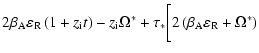
in the circuit of an "old"
loop in an active region begins to increase when "new" magnetic
flux emerges from under the photosphere. We have found that two
types of waves are generated in such a plasma due to the growth
of instabilities: the "kinetic Alfven-like" waves and new type of
waves, in the range of magnetoacoustic ones. The instability of
these latter waves has a clear threshold and it can be considered
as an "indicator" of the development of a preflare situation in an
active region.
Key words: plasmas - Sun: flares - Sun: chromosphere
Plasma instabilities are traditionally assumed to be one
of the main sources of waves in the flare atmosphere (Priest 1982;
Somov 1994; Zaitsev et al. 1994). Their hierarchy is usually
considered as an important element in the theory of cyclotron
maser emission (CME) (Melrose 1989; Zaitsev et al. 1994; Mel'nikov
et al. 2002) as well as in the dynamics of current sheets which
form in flaring arcades (Podgorny & Podgorny 2001), namely where
flares most frequently occur (De Jager 1959; Priest 1982). Thus
the loops of arcades are "post-flare" loops of a previous flare
and the preflare of the next one. The investigation of the
preflare plasma state on the basis of Heyvaerts-Priest-Rust (HPR)
theory (Heyvaerts et al. 1977; Podgorny & Podgorny 2001) is
current practice. In this theory a flare is considered to be the
result of the interaction of a "new" magnetic flux, which emerges
from under the photosphere and an "old" one, which passes through
a current circuit of a loop in an arcade. Such interaction results
in an adiabatic slow increase of the amplitude of a weak
quasi-static electric ("DC") field in the circuit of the "old"
loop. From general physical considerations (De Jager 1959;
Kadomtsev & Pogutse 1967) it is clear that, in such circumstances,
different low-energetic wave instabilities of the "stream" type
will grow in plasma. If the growth time of the large-scale
electric field amplitude
is much larger than the time of instability development, - this
situation occurs most frequently (Poletto & Kopp 1986), - then
the mechanism of "direct initiation" of instability by the
electric field will take place. The corresponding instabilities
will have a clearly expressed threshold character (Kryshtal &
Kucherenko 1995). The value of the amplitude
,
expressed in units of the local Dreicer field  ,
will be the threshold value in this case. We
assume that in preflare situation there are only very few
"super-energetic" charged particles (i.e. plasma "without beams").
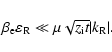
When the electric field is weak, i.e. when
,
will be the threshold value in this case. We
assume that in preflare situation there are only very few
"super-energetic" charged particles (i.e. plasma "without beams").
When the electric field is weak, i.e. when
 |
(1) |
the percentage of "runaway" electrons is so small that
their influence on the instability development can be regarded as
negligible (Alexandrov et al. 1988). Of course,this is only one of
the possible scenarios for the preflare situation development
(Zaitsev et al. 1994).
In connection with the "perpetual" problem of solar physics, the
problem of coronal heating, Aschwanden (2001) has formulated
interesting conclusions based on the recent soft X-ray and EUV data from space observations with the YOHKOH, SOHO and TRACE satellites. We consider that the inclusion of the chromosphere is
very important not only "in conventional AC and DC models"
(Aschwanden 2001) but in the investigation of the dynamics of the
preflare plasma state in a loop in general. Preferential footpoint
heating (Aschwanden 2001) can be explained from our point of view
in the framework of the well-known Ionson model (Ionson 1978). The
most important necessary condition is the generation of the
kinetic Alfven waves (KAW) on the "chromospheric floor" of the
loop current circuit. These waves propagate almost perpendicular
to the direction of the magnetic field
 of the
loop in its surface layer (Ionson 1978). Second, the observed
overdensity of order
of the
loop in its surface layer (Ionson 1978). Second, the observed
overdensity of order
 (Aschwanden 2001),
which, of course, is not less in the chromosphere, seems to be a
good reason to assume that strong gradients of the plasma density
can have a larger effect than the similar values of temperature and
magnetic field amplitude
(Aschwanden 2001),
which, of course, is not less in the chromosphere, seems to be a
good reason to assume that strong gradients of the plasma density
can have a larger effect than the similar values of temperature and
magnetic field amplitude
 .
Here
we denote by
.
Here
we denote by
![$\nabla_{L} \equiv \frac{{\partial}} {{\partial x}}{\left[{\ln n_{0}{_{\alpha}} (x)} \right]} \approx \frac{{1}}{{L_{\alpha}}}$](/articles/aa/full/2004/24/aa3594/img18.gif) the inverse of the gradient scale
the inverse of the gradient scale
 ,
,
 is the reduced spatial gradient of
density. The value of
is proportional to the inverse
value of the mean scale of the density inhomogeneity of the
electrons and ions (
is the reduced spatial gradient of
density. The value of
is proportional to the inverse
value of the mean scale of the density inhomogeneity of the
electrons and ions (
 ). Analogous values for the
temperature and the magnetic field can be introduced in a similar
way. Since the end of the 1950s (De Jager 1959), it is well known
that overdensity is the most distinguishing property of post-flare
loops. When the effect of the reduced spatial gradient of density
dominates, it is possible to neglect the shear influence on the
instability development. This needs some special condition
regarding the plasma state and the characteristics of the
perturbation. The increasing number of detections of flarelike
events at temperatures of
). Analogous values for the
temperature and the magnetic field can be introduced in a similar
way. Since the end of the 1950s (De Jager 1959), it is well known
that overdensity is the most distinguishing property of post-flare
loops. When the effect of the reduced spatial gradient of density
dominates, it is possible to neglect the shear influence on the
instability development. This needs some special condition
regarding the plasma state and the characteristics of the
perturbation. The increasing number of detections of flarelike
events at temperatures of
 MK in EUV (with
SOHO/ETT and TRACE) (Aschwanden 2001) allows us to assume that
the early stage of the preflare process can correspond to a
temperature of
MK in EUV (with
SOHO/ETT and TRACE) (Aschwanden 2001) allows us to assume that
the early stage of the preflare process can correspond to a
temperature of  0, 5 MK. The plasma parameters should be
obtained from the well-known semiempirical model of chromospheric
flare regions (Machado et al. 1980).
0, 5 MK. The plasma parameters should be
obtained from the well-known semiempirical model of chromospheric
flare regions (Machado et al. 1980).
We investigate the physical conditions for the growth of
low-frequency plasma wave instabilities in the case of the
long-wave perturbations propagating almost perpendicular to the
direction of the loop magnetic field
.
We use a
local rectangular Cartesian coordinate system with the Z-axis
directed along the field vectors
 and
(we assume that
and
(we assume that
 ). Taking into account that we consider a plasma in the "chromospheric floor" near the footpoint of a loop, this means that the XY-plane is actually parallel to
the surface of the photosphere. For intermediate calculations we
have used a cylindrical coordinate system in velocity space
(
). Taking into account that we consider a plasma in the "chromospheric floor" near the footpoint of a loop, this means that the XY-plane is actually parallel to
the surface of the photosphere. For intermediate calculations we
have used a cylindrical coordinate system in velocity space
(
 )
(Alexandrov et al. 1988).
)
(Alexandrov et al. 1988).
We assume that the plasma has a one-dimensional spatial gradient
of its density along the X-axis. The thickness of the surface
layer of the loop is the mean spatial scale of inhomogeneity of
the plasma density. For the local solutions of the dispersion
relation for the low-frequency plasma waves (Michailovsky 1963) we
consider that the origin of the Cartesian coordinates is placed
near the inner border of the surface layer. We assume
(Michailovsky 1963), that the wave frequency  satisfies the inequality
 |
(2) |
where
 is the local ion gyrofrequency.
In the present investigation, we use the same mechanism of "direct initiation" of instability and the same plasma model as in our previous work (Kryshtal & Kucherenko 1995; Kryshtal 2000), the
most important properties of which are the following:
- 1.
- The weak large-scale electric field
 is quasi-static, which implies that
![\begin{displaymath}%
{\frac{{\partial}} {{\partial t}}}{\left[ {\ln {\left\vert
...
...\vert}} \right]} \ll \tau _{{\rm inst}}^{ - 1}
\approx \gamma.
\end{displaymath}](/articles/aa/full/2004/24/aa3594/img31.gif) |
(3) |
This can be considered as typical for flares processes and for
different types of plasma instabilities (Zaitsev et al. 1994).
On the other hand there is observational evidence for a
correlation between the time of maximum E0 (t) and the
moment at which the first energy release occurs in a flare
(Poletto & Kopp 1986; Zaitsev et al. 1994). The left-hand side
of inequality (3) approximately equals the value
 ,
where
,
where  is the time for the amplitude E0 (t) to grow to its maximum value.
We assume that the electric field under consideration is extremely
weak and that the threshold value
 ,
at which the instability, with growth rate
,
at which the instability, with growth rate  and growth time
 ,
starts developing, does not much exceed the equilibrium value
,
starts developing, does not much exceed the equilibrium value
 .
This value corresponds to the
origin of the preflare process when interaction between the "old"
and "new" magnetic fluxes is absent. In this situation
equals the time of the short-period prediction of a flare and the instability appearance can be considered in a sense as a
"forerunner" of a flare process.
.
This value corresponds to the
origin of the preflare process when interaction between the "old"
and "new" magnetic fluxes is absent. In this situation
equals the time of the short-period prediction of a flare and the instability appearance can be considered in a sense as a
"forerunner" of a flare process.
- 2.
- As earlier (Kryshtal 2000) the plasma under consideration is
assumed to be fully ionized and collisions are described by a BGK model integral (Alexandrov et al. 1988). The equilibrium velocity distribution function for ions is assumed to be pure Maxwellian,
but the same function for the electrons is described by a shifted
Maxwellian distribution with electron shift velocity:
 |
(4) |
here,
 is the ion-electron collision frequency. When
a weak ("external") electric field exists and there is an enough
strong magnetic field in the plasma, the ion-electron collisions
dominate (Alexandrov et al. 1988).The contribution of other mutual
collisions of charged particles can be taken into account in a
phenomenological way with the help of the factor
is the ion-electron collision frequency. When
a weak ("external") electric field exists and there is an enough
strong magnetic field in the plasma, the ion-electron collisions
dominate (Alexandrov et al. 1988).The contribution of other mutual
collisions of charged particles can be taken into account in a
phenomenological way with the help of the factor
 (Kryshtal & Kucherenko 1995).
- 3.
- Taking into account the real scales of inhomogeneity of the
plasma (electron or ion) densities in the loops (Zaitsev et al. 1994) we consider the long-wave approximation for the perturbations:
 |
(5) |
where  and
and  are the electron and ion
kinetic parameters respectively,
are the electron and ion
kinetic parameters respectively,  is the transverse
component of perturbation wave-vector
is the transverse
component of perturbation wave-vector  (
(
 ;
;
 ),
),
 and
and
 are respectively
the electron and ion thermal velocities and
are respectively
the electron and ion thermal velocities and
 is
the electron gyrofrequency.
is
the electron gyrofrequency.
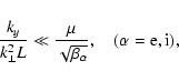
- 4.
- The spatial density inhomogeneity is supposedly "weak", which
means, according to Michailovsky (1963) that the conditions
 |
(6) |
where
![\begin{displaymath}%
\omega _{{\rm e,i}}^{ *} \equiv {\frac{{k_{y} \upsilon
_{T{...
...al}} {{\partial
x}}}{\left[ {\ln n_{0{\rm e,i}} (x)} \right]},
\end{displaymath}](/articles/aa/full/2004/24/aa3594/img52.gif) |
(7) |
have to be satisfied by the drift frequencies of electrons and ions, respectively.
- 5.
- We have used the condition of quasi-neutrality of plasma
 |
(8) |
for the equilibrium densities of the charged particles. When Eq. (8) is valid for an arbitrary x, the analogous equation for the spatial gradients of densities is also
valid:
 |
(9) |
Equation (9) allows us to make use of the well-known simple connection between the drift frequencies of electrons and ions (Michailovsky 1963; Alexandrov et al. 1988)
 |
(10) |
where
 |
(11) |
In our calculations we have assumed that the density profiles in the surface layer have the form
![\begin{displaymath}%
n_{0\alpha} (x) = n_{0} \exp {\left[ { -
{\frac{{x}}{{L_{\alpha}} } }} \right]}, \quad (\alpha = {\rm e},{\rm i})
\end{displaymath}](/articles/aa/full/2004/24/aa3594/img57.gif) |
(12) |
and that
 |
(13) |
is satisfied. In this case the condition (6) is practically equivalent to the well-known inequality (Michailovsky 1963; Kadomtsev & Pogutse 1967) for plasma with weak spatial
inhomogeneity of density
 |
(14) |
where
 is the ion gyroradius. Equation (14), as a rule, is easily satisfied in the loops (Zaitsev et al. 1994).
- 6.
- Under the mentioned above conditions, it is natural to make
in the calculation the local approximation to the dispersion
relation (DR), which is justified if (Michailovsky 1963)
 |
(15) |
where
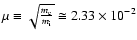 (for one-charged ions) and
 is the well-known "plasma
  ":
":
 |
(16) |
The local approximation to the DR allows us to neglect the influence of the boundaries on the process of instability development. Since we consider a "low-" plasma (Michailovsky 1963), then the following inequality has to be satisfied (Krall & Trivelpiece 1973)
 |
(17) |
We assume everywhere that
 |
(18) |
Then the condition (15) for the solutions to be local turns out to be even more stringent than the condition
 |
(19) |
for the transverse wave-length of the perturbation. Inequality (19) is the condition of the approximation of geometrical optics.
- 7.
- Taking into account the fact that in a surface layer the main spatial inhomogeneity of density is in the direction perpendicular to the magnetic field
,
as well as the fact that
the low-frequency waves under consideration are of a quasi-electrostatic type, we assume that the condition
 |
(20) |
is satisfied for the components of the perturbation wave-vector (Ionson 1978).
- 8.
- We take the "longitudinal" phase velocity of the perturbation to vary in the range
 |
(21) |
This range is typical of the "Alfven-like" and "drift-like" waves in a plasma (Krall & Trivelpiece 1973). We have also made use of some additional conditions:
- 9.
- In the case of "weak inhomogeneity" we consider a "moderately
nonisothermal" plasma with
 |
(22) |
On the one hand this allows one to neglect the possible influence of
ion-acoustic turbulence on the process of instability development.
Actually it means that
 |
(23) |
On the other hand, the relatively low values of t in (22) imply that threshold value
 ,
at which the instability arises, may be low too. This may be important for the problem of pre-heating of the loop foot-points (Aschwanden 2001).
,
at which the instability arises, may be low too. This may be important for the problem of pre-heating of the loop foot-points (Aschwanden 2001).
- 10.
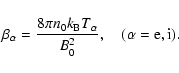
- We noted that we neglect in our calculations the reduced spatial gradients of temperature and
magnetic field compared to that of density. According to Kadomtsev & Pogutse, this is equivalent to the neglect of the influence of "shear" (Kadomtsev & Pogutse 1967). For a
characteristic scale of the perturbation of order
 ,
i.e. for
,
i.e. for
 ,
this assumption is
correct if the condition for the ion "plasma "
,
this assumption is
correct if the condition for the ion "plasma "
 |
(24) |
is satisfied. In Eq. (24)
 ,
where
,
where
 is
the Alfven velocity and
is
the Alfven velocity and
 is the ion plasma
frequency. The analogous condition for the electron "plasma " has the form
is the ion plasma
frequency. The analogous condition for the electron "plasma " has the form
 |
(25) |
Taking the conditions (5) and (20) into account, these last two inequalities, (24) and (25), point to the importance of the "right choice" of plasma parameters, i.e. appropriate values of the densities and temperatures of the electrons and ions. With the mentioned above restrictions and conditions, this is not so simple. Semiempirical models of the
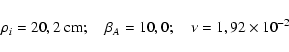
flare chromosphere (Machado et al. 1980) fortunately provide us with necessary parameters. In our calculations we used the following values:
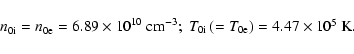 |
(26) |
We supposed that in the local thermodynamical equilibrium
 before the interaction of the "old" and "new" magnetic
fluxes, and
before the interaction of the "old" and "new" magnetic
fluxes, and  can exceed
  according to Eq. (22) in the case of weak inhomogeneity in the early stage of the preflare process. In the paper of Machado et al. (1980) the
values of
according to Eq. (22) in the case of weak inhomogeneity in the early stage of the preflare process. In the paper of Machado et al. (1980) the
values of
 and
correspond to the height h=1459 km above the photosphere. Strictly speaking the magnetic field amplitude in our model cannot be arbitrary. This is
clear in view of the conditions and approximations of the employed
model. There is still some freedom in the choice of this parameter
(Gopasyuk 1987). We assumed
and
correspond to the height h=1459 km above the photosphere. Strictly speaking the magnetic field amplitude in our model cannot be arbitrary. This is
clear in view of the conditions and approximations of the employed
model. There is still some freedom in the choice of this parameter
(Gopasyuk 1987). We assumed
 .
This value is
very closed to the value
.
This value is
very closed to the value
 from Aschwanden (1987).
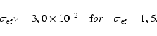
For such magnetic field amplitudes and with the parameters given in Eq. (26) and extremely small values of
 ,
the conditions (24) and (25) can be easily satisfied in the case of a weak inhomogeneity. In the opposite case of a strong inhomogeneity, for
extremely small values of
,
the conditions (24) and (25) can be easily satisfied in the case of a weak inhomogeneity. In the opposite case of a strong inhomogeneity, for
extremely small values of  ,
when instability can develop on the background of turbulence and the value of
can sharply increase, the conditions (24) and (25) practically determine an upper limit for
.
,
when instability can develop on the background of turbulence and the value of
can sharply increase, the conditions (24) and (25) practically determine an upper limit for
.
In the case of weak inhomogeneity, when the ion-electron collisions dominate, we can estimate for the parameters (26) the equilibrium value
,
which corresponds to the steady state in the loop circuit (without interaction of the "new" and "old" magnetic fluxes). If we assume that the loop under consideration is a "semitorus" with small radius R0, it can be shown that
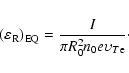 |
(27) |
For a current in this loop I = 1 
 (Gopasyuk 1987) and
 (Zaitsev et al. 1994), we then obtain
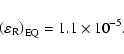 |
(28) |
Of course, it seems very problematic to obtain the exact value
of R0, so the estimate (28) can give only an order
of magnetude
.
The starting point for obtaining the dispersion relation (DR) for this plasma model is the expression for the scalar dielectric permeability of a hot magnetoactive plasma with
spatial inhomogeneity. (Alexandrov et al. 1988).
When the electric field in the low-frequency wave
in the inhomogeneous medium can be considered as quasi-potential,
the equation for this permeability in the inhomogeneous plasma,
 |
(29) |
plays the same role as the standard DR in homogeneous plasma. In this case, Eq. (29) can be considered as the eikonal equation for electrostatic waves in the zero order of
geometrical optics. For the low-frequency waves, which satisfy condition (2), Eq. (29) can be simplified in a standard way (Kryshtal 2000) and reduced to the form
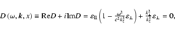 |
(30) |
where
 and
and
 are the longitudinal and transverse
parts of the dielectric permeability respectively, c is the
speed of light in vacuum. This form of DR was first investigated
by Michailovsky (1963) in the local approximation at
are the longitudinal and transverse
parts of the dielectric permeability respectively, c is the
speed of light in vacuum. This form of DR was first investigated
by Michailovsky (1963) in the local approximation at
 ,
,
 and t = 1. In the present plasma
model with
and t = 1. In the present plasma
model with
 ,
,
 and t>
1 the form of the DR remains the same (Kryshtal 2000), but, if we
take into account the existence of subdreicer field and the
influence of the collisions, additional terms appear in the
expressions of
and
.
These expressions become much more
complicated, with terms that describe the ion thermal motion. But
the DR becomes suitable for analysis when
takes extremely small values. This form of the DR, which is
modified by the presence of the external electric field, pair
Coulomb collisions and ion thermal motion, is refered to as the
modified dispersion relation (MDR). Each root of the equation
(Krall & Trivelpiece 1973)
and t>
1 the form of the DR remains the same (Kryshtal 2000), but, if we
take into account the existence of subdreicer field and the
influence of the collisions, additional terms appear in the
expressions of
and
.
These expressions become much more
complicated, with terms that describe the ion thermal motion. But
the DR becomes suitable for analysis when
takes extremely small values. This form of the DR, which is
modified by the presence of the external electric field, pair
Coulomb collisions and ion thermal motion, is refered to as the
modified dispersion relation (MDR). Each root of the equation
(Krall & Trivelpiece 1973)
 |
(31) |
corresponds to a certain kind of plasma wave, with dispersion law
 ,
where m is a number labeling the root. We consider this plasma wave as the solution of MDR. In the present plasma model,
,
where m is a number labeling the root. We consider this plasma wave as the solution of MDR. In the present plasma model,
 actually depends not on x, but on L(see Eqs. (12)
 (13)). We determine the growth rate (positive or negative) of the instability from the equation
 |
(32) |
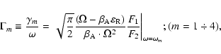
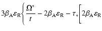
In the framework of our approximations, Eq. (31) can be reduced to the polynomial form
 |
(33) |
with
 |
|
|
(34) |
![\begin{displaymath}%
P_{3} = {\frac{{\Omega^{ *}} }{{t}}} - 2\beta _{\rm A}
\var...
...\Omega ^{ *} \left( {1 - {\frac{{1}}{{t}}}} \right)}
\right]},
\end{displaymath}](/articles/aa/full/2004/24/aa3594/img116.gif) |
(37) |
 |
(38) |
where
![\begin{displaymath}%
\tau _{\ast} = \sqrt {{\frac{{2\pi}} {{z_{\rm i} t}}}}
{\fr...
...rm ef}} \in {\left[ {1;2.5} \right]}}. \hfill \\
\end{array}}
\end{displaymath}](/articles/aa/full/2004/24/aa3594/img118.gif) |
(39) |
In the Eq. (33)
 |
(40) |
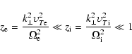
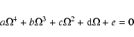
is the reduced frequency (or reduced "longitudinal" phase velocity). At the same time in the Eqs. (34)(38)
 |
(41) |
where
 |
(42) |
are the reduced drift frequencies of the charged particles. In this paper we only investigated the real roots of the algebraic equation of the fourth order (33), because
we want to exclude the possible cases of "aperiodic" instability
or "aperiodic" damping (Alexandrov et al. 1988). In numerical
simulations, we have found that complex roots of Eq. (33) appear at
 .
This is why we have taken
.
This is why we have taken
 as the upper limit of the
interval in (39).
as the upper limit of the
interval in (39).
Equation (33) can be solved by the standard Euler method, but for extremely small values of
(actually as
 )
it becomes impossible to
obtain the solution in an analytical form. So, we had to make use
of the numerical calculations based on exact formulae (Mishina & Proskuryakov 1962). We have used the roots of the resolvent equation. For all roots to be real and positive, and thus to
obtain all four roots of the MDR (33) as real, the condition
)
it becomes impossible to
obtain the solution in an analytical form. So, we had to make use
of the numerical calculations based on exact formulae (Mishina & Proskuryakov 1962). We have used the roots of the resolvent equation. For all roots to be real and positive, and thus to
obtain all four roots of the MDR (33) as real, the condition
 |
(43) |
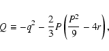
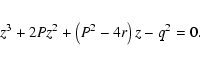
should be satisfied for the discriminant D of the resolvent equation (Mishina & Proskuryakov 1962). Here the following notations have been used:
where P, q and r are the coefficients of the fourth order equation in the reduced form
y4 - Py2 + qy + r = 0.
This equation can be obtained from the initial equation
through the standard transformation
The resolvent equation of the third order has the form
Equation (43) imposes the most stringent restrictions on the main
plasma characteristics of the employed model. However, these
restrictions allow us to consider separately the cases of the
"weak" and "strong" inhomogeneities.
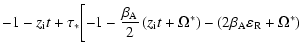
The obtained real roots of the MDR (33) have to be substituted into formula (32) to analyse the expressions for the growth rates. Only if
 |
(44) |
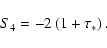
the corresponding waves grow during the linear stage of the process of instability development. The reduced growth rates for the all four roots of the MDR (33) have the following form:
 |
(45) |
with
 |
(46) |
 |
(47) |
where
 |
(48) |
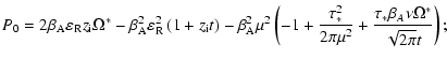
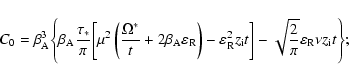
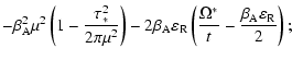
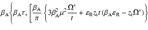
| C1 |
= |
![$\displaystyle \beta_{\rm A}^{2} \Biggl\{\sqrt{\frac{8}{\pi}} \nu \left[\varepsi...
...}\left(\frac{\Omega^{*}}{2t} - \beta_{\rm A} \varepsilon _{\rm R}\right)\right]$](/articles/aa/full/2004/24/aa3594/img136.gif) |
|
| |
|
![$\displaystyle + \beta_{\rm A}\frac{\tau_{*}}{\pi} \left[\beta_{\rm A} \mu ^{2}\...
...ft\{\pi \Omega^{*} - z_{\rm i} t\left(1 + \pi \right) \right\}
\right]\Biggl\};$](/articles/aa/full/2004/24/aa3594/img137.gif) |
(49) |
 |
|
|
(52) |
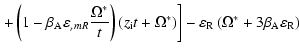
 |
(53) |
| S2 |
= |
 |
|
| |
|
![$\displaystyle + \Omega ^{ * }\left(1 - \frac{1}{t}\right) \biggl] + \sqrt{\frac{\pi}{2}} \nu \Omega ^{ *}\Biggl\};$](/articles/aa/full/2004/24/aa3594/img154.gif) |
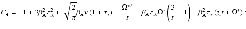
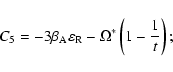
(57) |
![\begin{displaymath}S_{3} = 6\beta _{\rm A} \varepsilon _{\rm R} - \frac{\Omega^{...
...c{1}{t}\right)\right] - \sqrt{\frac{\pi}{2}} \nu \Omega ^{ *};
\end{displaymath}](/articles/aa/full/2004/24/aa3594/img155.gif) |
(58) |
 |
(59) |
Numerical simulation has shown that the requirement of the absence of an imaginary part in the roots of MDR (33) has to be supplemented by the condition
 |
(60) |
Practically, this means that the use of the linear approximation of perturbation theory is valid. These two conditions (43) and (60) allow us to consider separately the cases of "weak" and "strong" inhomogeneity. The case of weak inhomogeneity corresponds to extremely small values of
and extremely large possible values of
and .
At the same time the conditions (5) and (20) hold for
and
respectively, as well as condition (22) for t. Specifically, we assumed that the parameters
,
t,
and
vary in the following ranges:
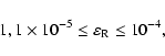 |
(61) |
 |
(62) |
 |
(63) |
 |
(64) |
By analogy with
we designated the value of t at which the growth rate becomes positive by
 .
.
For the set of parameters (26) and
we have
 |
(65) |
and
 |
(66) |
In the framework of our model, the need for a numerical solution evidently increases. For very narrow intervals of variations of
and
and constant values
 and
and
 ,
corresponding areas on the surfaces of the
reduced longitudinal phase velocities
,
corresponding areas on the surfaces of the
reduced longitudinal phase velocities
 are practically flat. Their local
"topology" (i.e. existence of the local extrema) does not play any
significant role. In this situation the specific ranges for
and ,
where condition (43) is satisfied, as well as specific orientation in "parameter space" of
these "locally flat" surfaces, seem much more important, because
they allow us to determine, in principle, the dispersion law, i.e.
the type of plasma wave. Strictly speaking, this is just an
estimate, but this estimate turns out to be reasonably good.
are practically flat. Their local
"topology" (i.e. existence of the local extrema) does not play any
significant role. In this situation the specific ranges for
and ,
where condition (43) is satisfied, as well as specific orientation in "parameter space" of
these "locally flat" surfaces, seem much more important, because
they allow us to determine, in principle, the dispersion law, i.e.
the type of plasma wave. Strictly speaking, this is just an
estimate, but this estimate turns out to be reasonably good.
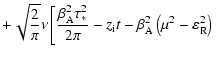
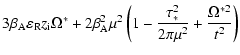
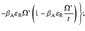
The calculations show that four roots of the MDR (33) can
be formally split into two pairs. The roots, which we call
"
 -" and "
 -waves", have in the ranges
(61)(64) very close (but not the same)
values of
-waves", have in the ranges
(61)(64) very close (but not the same)
values of
 and
and
 ,
but opposite signs (
is positive
and
is negative). The
-wave can be
easily interpreted as the "right" (i.e. with kz > 0) kinetic
Alfven wave, modified by the pair collisions and large-scale
subdreicer electric field. Unfortunately, we cannot interpret the
-wave in the same way as the inverse kinetic
Alfven wave. In the framework of the present model we have used in calculations
only
and
,
but opposite signs (
is positive
and
is negative). The
-wave can be
easily interpreted as the "right" (i.e. with kz > 0) kinetic
Alfven wave, modified by the pair collisions and large-scale
subdreicer electric field. Unfortunately, we cannot interpret the
-wave in the same way as the inverse kinetic
Alfven wave. In the framework of the present model we have used in calculations
only
and
 as variable parameters to
obtain the maximum effect. We do not know the details of the
polarization of perturbation, so, we cannot say whether the
negative values of
are the result of
incompleteness of our description of perturbation, or whether they
demonstrate the well-known "parasitic" effect, when negative
frequencies appear in DR (Michailovsky 1963; Alexandrov et al.
1988). For the same reason in the other pair of roots we consider
only the
as variable parameters to
obtain the maximum effect. We do not know the details of the
polarization of perturbation, so, we cannot say whether the
negative values of
are the result of
incompleteness of our description of perturbation, or whether they
demonstrate the well-known "parasitic" effect, when negative
frequencies appear in DR (Michailovsky 1963; Alexandrov et al.
1988). For the same reason in the other pair of roots we consider
only the
 -wave (with positive values) and suppose
that only this root corresponds to a "real" wave. It is hard
enough to determine exactly the dispersion law for this wave. We
can only approximately describe it as a wave from the range of the
slow magneto-acoustic ones, because in our model the dispersion
law for these SMA-waves has the approximate form
-wave (with positive values) and suppose
that only this root corresponds to a "real" wave. It is hard
enough to determine exactly the dispersion law for this wave. We
can only approximately describe it as a wave from the range of the
slow magneto-acoustic ones, because in our model the dispersion
law for these SMA-waves has the approximate form
 .
This wave is definitely modified by the weak
drift motions, pair Coulomb collisions and subdreicer electric
field. It practically does not depend on
(more exactly,
this dependence is very weak) and depends on
in an unusual way in comparison to KAW. This last fact
does not permit us to consider this
-wave as the
"exact" SMA-wave, even taking into account the corrections to the
dispersion law due to the collisions, subdreicer field and drift
motions. Here we meet an interesting phenomenon: at
,
t = 1 and
("Michailovsky's"-case, 1963), without the collisions and electric field, the DR (33) becomes a polynomial of third order. The roots of
this DR are the two Alfven (in our case - the kinetic Alfven)
waves and slow drift-Alfven wave (which contains in its dispersion
law the drift frequency (41)(42) as the
factor, and because of this is very slow) (Michailovsky 1963).
When
,
t > 1 and
,
the KAWs are, of course, modified, but remain KAWs. At the same
time the slow drift Alfven wave vanishes, and instead of this the
.
This wave is definitely modified by the weak
drift motions, pair Coulomb collisions and subdreicer electric
field. It practically does not depend on
(more exactly,
this dependence is very weak) and depends on
in an unusual way in comparison to KAW. This last fact
does not permit us to consider this
-wave as the
"exact" SMA-wave, even taking into account the corrections to the
dispersion law due to the collisions, subdreicer field and drift
motions. Here we meet an interesting phenomenon: at
,
t = 1 and
("Michailovsky's"-case, 1963), without the collisions and electric field, the DR (33) becomes a polynomial of third order. The roots of
this DR are the two Alfven (in our case - the kinetic Alfven)
waves and slow drift-Alfven wave (which contains in its dispersion
law the drift frequency (41)(42) as the
factor, and because of this is very slow) (Michailovsky 1963).
When
,
t > 1 and
,
the KAWs are, of course, modified, but remain KAWs. At the same
time the slow drift Alfven wave vanishes, and instead of this the
 -waves appear, which contain the drift frequency (41)(42) in their dispersion laws not as the small factor, but as the small correction. Figures 1 and 2
show the behaviour of the functions
-waves appear, which contain the drift frequency (41)(42) in their dispersion laws not as the small factor, but as the small correction. Figures 1 and 2
show the behaviour of the functions
 and
and
 at
at
 |
(67) |
 |
(68) |
Figures 3 and 4 show the behaviour of the corresponding reduced
growth rates
 and
and
 at the same values of
and
as in (67)(68). It can
be easily seen that
at the same values of
and
as in (67)(68). It can
be easily seen that
 ,
thus the
-wave (modified KAW) damps. At the same time
,
thus the
-wave (modified KAW) damps. At the same time
 becomes positive for some values of
and ,
when
becomes positive for some values of
and ,
when
 and
and
 .
This means that the instability of the
-wave has a clearly expressed threshold and can be considered as being an indicator of the
dynamics of preflare process. In a sense the generation of the
-wave during the linear stage of the process of instability development can be considered as a forerunner of a
flare in a loop structure.
.
This means that the instability of the
-wave has a clearly expressed threshold and can be considered as being an indicator of the
dynamics of preflare process. In a sense the generation of the
-wave during the linear stage of the process of instability development can be considered as a forerunner of a
flare in a loop structure.
![\begin{figure}
\par\includegraphics[width=8.8cm,clip]{ms3594f7.eps}\end{figure}](/articles/aa/full/2004/24/aa3594/Timg192.gif) |
Figure 7:
The growth rate of the inverse KAW-like instability
 at
at
 and
and
 . . |
| Open with DEXTER |
![\begin{figure}
\par\includegraphics[width=8.8cm,clip]{ms3594f8.eps}\end{figure}](/articles/aa/full/2004/24/aa3594/Timg193.gif) |
Figure 8:
The growth rate of inverse SMAW-like instability
 at
and
.
at
and
. |
| Open with DEXTER |
An interesting situation occurs for kz < 0. The
- and
 -waves become the physical meaningful ones, and
 -waves in a sense lose their physical meaning. Figures 5 and 6 show the behaviour of the inverse KAW-like
-wave and
the inverse SMAW-like
-wave.Their growth rates
-waves in a sense lose their physical meaning. Figures 5 and 6 show the behaviour of the inverse KAW-like
-wave and
the inverse SMAW-like
-wave.Their growth rates
 and
and
 are shown in Figs. 7 and 8. In this case the
-wave plays the role of a forerunner
of a flare. But it has one very important defect: at the same value of
are shown in Figs. 7 and 8. In this case the
-wave plays the role of a forerunner
of a flare. But it has one very important defect: at the same value of
 it has too high value of
.
In the framework of our model this is important.
it has too high value of
.
In the framework of our model this is important.
The role of magneto-acoustic waves in the flare models (Priest 1982; Somov
1994; Zaitsev et al. 1994; Zaitsev & Stepanov 1982), especially in the laboratory modelling of this phenomenon (Somov 1994; Zaitsev et al. 1994), is well-known. There is a considerable
number of investigations (Rosenraukh & Stepanov 1988; Terekhov et al. 2002; Zaitsev & Stepanov 1989) of the pulsations of the flare emission as well as investigations of the transverse waves
in the loop structures (Podgorny & Podgorny 2001; Mel'nikov et al. 2002; Schrijver et al. 2002). From our point of view, the most interesting peculiarities of the present plasma model and of the
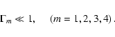
results that we have obtained are the following:
- 1.
- The instability is of a "non-beam" type. The only analogue of any kind of a beam in
this plasma model is the "beam" of "runaway" electrons. Due to the extremely small values of
in the case of weak inhomogeneity its influence on the process of instability
development is negligible.
- 2.
- The extremely small value of
from (68) points to the fact that we really study a very early stage of the preflare process (see
from (28)).
- 3.
- The relatively small value of
from (67) demonstrates that in the framework of this plasma model no considerable preheating near the foot-points is needed
for the generation of an
-wave.
- 4.
- The small values of the reduced growth rate
definitely
point to the fact that we study a clearly expressed wave process,
with a large number of periods of the generated waves.
Evidently, the generation of an
-wave is not enough for the real short-time prediction of a flare in a loop structure. But it is one of its most important necessary conditions.
Acknowledgements
The authors thank Dr. K. V. Alikajeva and Prof. S. I. Gopasyuk for useful discussions of the present work.
-
Alexandrov, A. F., Bogdankevich, L. S., & Rukhadze, A. A. 1988,
Principles of Plasma Electrodynamics, Higher School, Moscow,
Vys'shaya shkola
(In the text)
-
Aschwanden, M. I. 1987, Sol. Phys., 111, 113 [NASA ADS] (In the text)
-
Aschwanden, M. I. 2001, ApJ, 560, 1035 [NASA ADS] [CrossRef] (In the text)
- De
Jager, C. 1959, Structure and Dynamics of the Solar Atmosphere
(Springer)
-
Gopasyuk, S. I. 1987, Res. Sci. Tech., Ser. Astron. (USSR), 34,
6
(In the text)
-
Heyvaerts, I., Priest, E. R., & Rust, D. 1977, ApJ, 216,
213 [NASA ADS] (In the text)
- Ionson, J.
A. 1978, ApJ, 226, 650 [NASA ADS] [CrossRef] (In the text)
-
Kadomtsev, B. B., & Pogurse, O. I. 1967, in Problems of Plasma
Theory (USSR), ed. M. A. Leontovich, 5, 209
(In the text)
- Krall, N. A.,
& Trivelpiece, A. W. 1973, Principles of plasma Physics
(McGraw-Hill)
(In the text)
-
Kryshtal, A. N., & Kucherenko, V. P. 1995, J. Plasma Phys., 53,
169 [NASA ADS] (In the text)
-
Kryshtal, A. N. 2000, Kinemat. Phys. Celest. Bod., 16(6), 526
(In the text)
- Machado,
M. E., Avrett, E. H., Vernazza, J. E., & Noyes, R. W. 1980,
ApJ, 242, 236 [NASA ADS] (In the text)
- Mel'nikov, V. F.,
Fleishman, G. D., Fu, K. D., & Huang, G.-L. 2002, Sov. Astron.
- AJ, 79(6), 551
- Melrose,
D. B. 1989, Sol. Phys., 119, 143 [NASA ADS] (In the text)
-
Michailovsky, A. B. 1963, in Problems of Plasma Theory (USSR), ed.
M. A. Leontovich, 3, 141
(In the text)
- Mishina,
A. P., & Proskuriakov, I. V. 1962, Higher Algebra, MPPML,
Moscow (in Russian)
(In the text)
-
Podgorny, A. I., & Podgorny, I. M. 2001, Sov. Astron. - AJ,
78(1), 71
(In the text)
- Poletto,
G., & Kopp, R. A. 1986, in The Lower Atmosphere of Solar
Flares, Sacramento Peak, ed. D. F. Neideg, 453
(In the text)
- Priest, E.
R. 1982, Solar Magnetohydrodynamics (D. Reidel Publ.Co.)
(In the text)
- Somov, B. V.
1994, Fundamentals of Cosmic Electrodynamics (Kluwer Acad.
Publ.)
(In the text)
-
Schrijver, C. I., Ashwanden, M. I., & Title, A. M. 2002, Sol.
Phys., 206, 69 [NASA ADS] [CrossRef] (In the text)
-
Rosenraukh, Yu. M., & Stepanov, A. V. 1988, Sov. Astron. - AJ,
65, 300 [NASA ADS] [MathSciNet] (In the text)
-
Terekhov, O. V., Shevchenko, A. V., Kuz'min, A. G., et al. 2002,
Sov. Astron. Lett., 28, 6 [NASA ADS], 452
(In the text)
- Zaitsen,
V. V., & Stepanov, A. V. 1982, Sov. Astron. Lett., 8, 4 [NASA ADS],
248
(In the text)
- Zaitsen,
V. V., & Stepanov, A. V. 1989, Sov. Astron. Lett., 15, 2 [NASA ADS],
154
(In the text)
- Zaitsen,
V. V., Stepanov, A. V., & Tsap, Yu. T. 1994, Kinemat. Phys.
Celest. Bod., 10(6), 3
(In the text)
Copyright ESO 2004
![$\displaystyle + \beta_{\rm A} \varepsilon_{\rm R} \left(\beta_{\rm A} \varepsil...
...right) \biggl] + \beta_{\rm A}^{2} \varepsilon_{\rm R}^{2}\frac{\Omega^{ *}}{t}$](/articles/aa/full/2004/24/aa3594/img111.gif)
![$\displaystyle - \beta_{\rm A}^{2} \mu
^{2}\left[\tau_{*} \beta_{\rm A} \nu - \left(1 - \frac{\tau_{*}^{2}}{2\pi \mu^{2}}\right)\frac{\Omega ^{*}}{t} \right];$](/articles/aa/full/2004/24/aa3594/img112.gif)
![$\displaystyle \times \left(\frac{\Omega^{*}}{t} - \frac{\beta_{\rm A} \varepsil...
...R}\left(\beta_{\rm A} \varepsilon_{\rm R} + \frac{\Omega^{ *}}{2}\right)\biggl]$](/articles/aa/full/2004/24/aa3594/img114.gif)


![$\displaystyle \left. + \beta _{\rm A} \varepsilon _{\rm R} \tau _{*} \left(\beta_{\rm A} \varepsilon _{\rm R} + \frac{\Omega^{*}}{2}\right)\right]\Biggl\};$](/articles/aa/full/2004/24/aa3594/img141.gif)
![$\displaystyle \beta_{\rm A}^{2} \tau _{*} \left[\left(\frac{\Omega^{*}}{t} - \b...
...\left(2\beta _{\rm A} \mu ^{2} - \varepsilon _{\rm R} z_{\rm i} t\right)\right]$](/articles/aa/full/2004/24/aa3594/img142.gif)
![$\displaystyle - \sqrt{\frac{2}{\pi}} \beta_{\rm A} \nu \left[2\beta _{\rm A} \v...
...u _{*} \left(2\beta _{\rm A} \varepsilon _{\rm R} + \Omega ^{ *}\right)\right];$](/articles/aa/full/2004/24/aa3594/img144.gif)
![$\displaystyle +\tau _{ *} \Biggl\{\sqrt{\frac{2}{\pi}} \beta _{\rm A}^{3} \nu \...
...{\Omega ^{ *}}{2} + z_{\rm i} t \right) - \mu ^{2}\frac{\Omega ^{ *}}{t}\right]$](/articles/aa/full/2004/24/aa3594/img148.gif)
![$\displaystyle - z_{\rm i} \Omega ^{ *} - \beta _{\rm A}^{2} \frac{\Omega ^{*}}{...
... R}^{2} + \mu ^{2}\left(1 - \frac{\tau _{ *} ^{2}}{2\pi \mu ^{2}}\right)\right]$](/articles/aa/full/2004/24/aa3594/img150.gif)
![$\displaystyle +\tau _{ *} \Biggl\{\Omega ^{ *} \left[1 + \beta _{\rm A}
\vareps...
...}\left(3\beta _{\rm A} \varepsilon _{\rm R} + \Omega ^{*}\right)\right\}\right]$](/articles/aa/full/2004/24/aa3594/img151.gif)
![$\displaystyle + \sqrt{\frac{2}{\pi}} \beta _{\rm A} \nu \left[\beta _{\rm A}
\v...
...+ \frac{3}{2}\Omega ^{ *}\right) - \beta _{\rm A}^{2} \mu ^{2} \right]\Biggl\};$](/articles/aa/full/2004/24/aa3594/img152.gif)
![\begin{figure}
\par\includegraphics[width=8.8cm,clip]{ms3594f1.eps}\end{figure}](/articles/aa/full/2004/24/aa3594/img186.gif)
![\begin{figure}
\par\includegraphics[width=8.8cm,clip]{ms3594f2.eps}\end{figure}](/articles/aa/full/2004/24/aa3594/img187.gif)
![\begin{figure}
\par\includegraphics[width=8.8cm,clip]{ms3594f3.eps}\end{figure}](/articles/aa/full/2004/24/aa3594/img188.gif)
![\begin{figure}
\par\includegraphics[width=8.8cm,clip]{ms3594f4.eps} \end{figure}](/articles/aa/full/2004/24/aa3594/img189.gif)
![\begin{figure}
\par\includegraphics[width=8.8cm,clip]{ms3594f5.eps} \end{figure}](/articles/aa/full/2004/24/aa3594/img190.gif)
![\begin{figure}
\par\includegraphics[width=8.8cm,clip]{ms3594f6.eps}\end{figure}](/articles/aa/full/2004/24/aa3594/img191.gif)
![\begin{figure}
\par\includegraphics[width=8.8cm,clip]{ms3594f7.eps}\end{figure}](/articles/aa/full/2004/24/aa3594/img192.gif)
![\begin{figure}
\par\includegraphics[width=8.8cm,clip]{ms3594f8.eps}\end{figure}](/articles/aa/full/2004/24/aa3594/img193.gif)