A&A 420, L15-L18 (2004)
DOI: 10.1051/0004-6361:20040154
G. T. Birk1 - H. Lesch1 - C. Konz2
1 - Institut für Astronomie and Astrophysik,
Universität München, Scheinerstr 1, 81679 München, Germany
2 -
Max-Planck-Institute for Plasma Physics, Garching, Germany
Received 9 February 2004 / Accepted 28 April 2004
Abstract
The Earth is a planet with a dipolar
magnetic field which is
agitated by a magnetized plasma wind
streaming from the Sun. The magnetic field
shields the Earth's surface
from penetrating high energy solar wind particles, as well as
interstellar cosmic rays. The magnetic dipole has reversed sign
some hundreds of times over the last 400 million
years. These polarity reversals correspond to drastic breakdowns
of the dynamo action. The question arises what the consequences
for the Earth's atmosphere, climate, and, in particular, biosphere are.
It is shown by kinematic estimates and three-dimensional
plasma-neutral gas simulations
that the solar wind can induce very fast a magnetic field in the
previously completely unmagnetized Earth's
ionosphere that is strong enough to protect Earth from cosmic
radiations comparable to the case of an intact magnetic dynamo.
Key words: Earth - solar wind - solar-terrestrial relations - magnetic fields - magnetohydrodynamics
Paleomagnetic records show that the magnetism of Earth has
reversed itself hundreds of times over the last 400 million
years (Valet & Meynardier 1993; Juarez et al. 1998; Gee et al. 2000; Selkin
& Tauxe 2000; Valet 2003).
In fact, geomagnetic polarity
reversals represent the most dynamic feature of the Earth's magnetic
field. The polarity reversals do not occur instantaneously. Rather,
transition periods, that span some thousand years and are characterized
by unstable varying magnetic fields with no clear shape, lay between the
stable dipole field states.
During the transition periods the magnetic field strength can drop
well below 10![]() of the average value (Juarez et al. 1998; Guyodo &
Valet 1999; Selkin & Tauxe 2000)
which signifies a drastic breakdown of the Earth's dynamo.
In the present time the magnetic south pole has wandered over more than
1100 km during the last 200 years. The strength of the Earth's field
has decreased by
of the average value (Juarez et al. 1998; Guyodo &
Valet 1999; Selkin & Tauxe 2000)
which signifies a drastic breakdown of the Earth's dynamo.
In the present time the magnetic south pole has wandered over more than
1100 km during the last 200 years. The strength of the Earth's field
has decreased by ![]() per century. This decrease is by far the
fastest that has been verified since the last total field reversal, the
end of the so-called Matuyama chron, 730 000 years ago.
Also, by statistical estimates the Earth's dynamo is overdue for a reversal.
Thus, we have to expect a transition period characterized by a very
small Earth's magnetic field in the near future. Since the Earth's
dipole field provides us with a shield against cosmic rays and solar
high-energy radiation one may wonder about the consequences for life
on Earth.
Also, having in mind that Mars lost the atmosphere almost completely
after the final breakdown of the magnetic field (Luhmann & Bauer 1992),
one may speculate that
stripping by the solar wind could alter the Earth's atmosphere.
Severe climate changes could result.
Interesting enough, during the last Brunhes-Matuyama reversal,
no major changes in plant and animal life have been
detected. This may be partly due to the fact that the atmospheric
layers block some fraction of the cosmic radiation by scattering.
On the other hand, the
cosmogenic radionuclide production varies at least over the last
200 000 years as function of short-term variations of the magnetic
field (Frank 2000).
per century. This decrease is by far the
fastest that has been verified since the last total field reversal, the
end of the so-called Matuyama chron, 730 000 years ago.
Also, by statistical estimates the Earth's dynamo is overdue for a reversal.
Thus, we have to expect a transition period characterized by a very
small Earth's magnetic field in the near future. Since the Earth's
dipole field provides us with a shield against cosmic rays and solar
high-energy radiation one may wonder about the consequences for life
on Earth.
Also, having in mind that Mars lost the atmosphere almost completely
after the final breakdown of the magnetic field (Luhmann & Bauer 1992),
one may speculate that
stripping by the solar wind could alter the Earth's atmosphere.
Severe climate changes could result.
Interesting enough, during the last Brunhes-Matuyama reversal,
no major changes in plant and animal life have been
detected. This may be partly due to the fact that the atmospheric
layers block some fraction of the cosmic radiation by scattering.
On the other hand, the
cosmogenic radionuclide production varies at least over the last
200 000 years as function of short-term variations of the magnetic
field (Frank 2000).
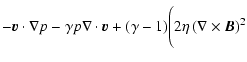
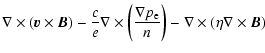
In this contribution. we consider the interaction of the solar wind with a completely unmagnetized Earth. When the solar wind encounters unmagnetized objects, such as Venus (Luhmann 1995) and comets (Konz et al. 2004), magnetic barriers and ionopauses develop. Although the interaction of a fully ionized and a weakly ionized gas is very complex, an important characteristic can be identified - the generation of magnetic fields caused by relative plasma-neutral gas shear flows. It has been shown (Huba & Fedder 1993) that this process operates in the Venus' ionosphere and is responsible for the non-dipole magnetic field measured there. The same process has been studied in detail for the generation of seed magnetic fields in emerging galaxies (Wiechen et al. 1998; Birk et al. 2002) and in circumstellar disks (Birk et al. 2003). A kinematic estimate indicates that relatively strong magnetic fields are generated in the Earth's ionosphere. So far, the only way to study the dynamical non-linear interaction of the magnetized fully ionized solar wind plasma and the partially ionized Earth's ionosphere are three-dimensional plasma-neutral gas simulations. Our numerical studies show the draping of the magnetic field of the solar wind and the self-generation of a relatively strong magnetic field in the Earth's ionosphere.
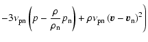
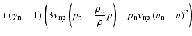
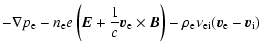
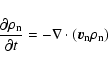
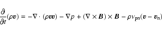
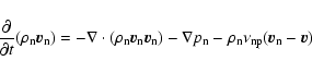
The interaction of a fully ionized plasma with a partially ionized gas
can be described by the fluid balance equations for the mass densities,
momentum densities and thermal pressures of the different species (see
Sect. 3) together with the generalized Ohm's law. Ohm's law connects the
electric fields
and electric currents in a plasma. For the low-frequency dynamics we are
interested in, it can be deduced from the
inertialess electron momentum equation (Mitchner & Kruger 1973; Wiechen et al. 1998)
For the parameters given, a field strength comparable to the present dipole value is generated after only ten minutes in the ionosphere. Thus, magnetic fields can be generated very efficiently around the unmagnetized Earth.
The interaction of the solar wind with the Earth's ionosphere can be
modeled by a plasma-neutral gas two fluid description.
In our simulations, the following normalized plasma-neutral gas equations are numerically integrated
Figure 1 shows an arrow plot of the solar wind velocity field at three
different times (t=30 s; upper plot, t=60 s; middle plot
and t=600 s; lower plot).
The wind encounters the Earth and is deflected around
the planet.
![\begin{figure}
\par\includegraphics[width=7.7cm,clip]{Gb091_f1a.eps}\par\vspace*...
...\par\vspace*{3mm}
\includegraphics[width=7.7cm,clip]{Gb091_f1c.eps}
\end{figure}](/articles/aa/full/2004/23/aagb091/img57.gif) |
Figure 1: The solar wind flow around the Earth in the z=0-plane at t=30 s ( upper plot), t=60 s ( middle plot) and t=600 s ( lower plot). |
| Open with DEXTER | |
The magnetic field lines carried by the solar wind are draped around
the Earth (Fig. 2). The draping leads to an amplification of the
magnetic field near the Earth by one order of magnitude. This effect
is well known, e.g., from investigations on the interaction of the solar wind
with the unmagnetized Venus (Russel 1993; Luhmann 1995).
![\begin{figure}
\par\includegraphics[width=8.2cm,clip]{Gb091_f2.ps}
\end{figure}](/articles/aa/full/2004/23/aagb091/img58.gif) |
Figure 2: The draping of the magnetic field lines of the solar wind around the Earth at t=600 s. |
| Open with DEXTER | |
Close to the Earth, the momentum transfer between the
charged particles of the solar wind and the neutrals of the Earth's
ionosphere becomes important
(see final terms in Eqs. (7) and (8)).
Consequently, a new strong non-dipole
magnetic field is generated by the sheared relative
plasma-neutral gas motion (see final term in Eq. (9)).
Parameter studies show the kinematic finding (see Sect. 2) that the
strength of the generated magnetic field depends on the shear length L. The maximum shear length is fixed in the simulation by an appropriate
choice of the profile for
![]() .
For a shear length L=10 km a magnetic field of about the present
dipole strength (
.
For a shear length L=10 km a magnetic field of about the present
dipole strength (
![]() G) is induced in the
ionosphere after about 10 min (Fig. 3).
For a given L the time scale of the
field generation
G) is induced in the
ionosphere after about 10 min (Fig. 3).
For a given L the time scale of the
field generation ![]() results from the dynamics.
The field is generated
in heights of some hundreds of
kilometers all around the Earth with the exception of the
subsolar region where the magnetic field is weaker.
If the shear length were chosen as say 100 km, the maximum of the generated
field strength would be
results from the dynamics.
The field is generated
in heights of some hundreds of
kilometers all around the Earth with the exception of the
subsolar region where the magnetic field is weaker.
If the shear length were chosen as say 100 km, the maximum of the generated
field strength would be
![]() G.
G.
We find that the draping effect is much weaker than the magnetic field
self-generation by the shear flow.
![\begin{figure}
\par\includegraphics[width=7.2cm,clip]{Gb091_f3.eps}
\end{figure}](/articles/aa/full/2004/23/aagb091/img61.gif) |
Figure 3: The strength of the induced magnetic field in the Earth's ionosphere at t=500 s. |
| Open with DEXTER | |
We studied the interaction of the magnetized fully ionized solar wind plasma with the unmagnetized partially ionized Earth's ionosphere. When the solar wind hits the Earth the magnetic field lines carried along with it are draped around the planet. What is more important, the relative motion between the solar wind plasma and the ionosphere results in the self-generation of magnetic fields in the ionospheric layer. The strengths of these fields depend on the shear length of the relative flows, which, in contrast to the other relevant physical parameters, is not well known. For a reasonable shear length of L=10 km the maximum strength of the newly generated magnetic field is comparable to the one of the present dipole field. Consequently, even in the case of a complete breakdown of the Earth's dynamo, the biosphere is still shielded against cosmic rays, in particular coming from the sun, by the magnetic field induced by the solar wind.

![$\displaystyle 5\times 10^{-4}~ {\rm G} \left[\frac{\nu_{\rm en}}{200
\ {\rm Hz}...
...\rm SW}}{450 \ {\rm km/s}}\right]
\left[\frac{L}{10\ {\rm km}}\right]^{-1} \tau$](/articles/aa/full/2004/23/aagb091/img36.gif)

![\begin{displaymath}{{\partial {\vec{B}}} \over {\partial t}} = \nabla \times ({\...
...abla \times [\hat\nu_{\rm en} ({\vec{v}}_{\rm n} - {\vec{v}})]
\end{displaymath}](/articles/aa/full/2004/23/aagb091/img43.gif)