A&A 419, 837-848 (2004)
DOI: 10.1051/0004-6361:20034421

The 2-8 keV cosmic X-ray background spectrum as observed with XMM-Newton^,

A. De Luca^1,2 - S. Molendi¹

1 - Istituto di Astrofisica Spaziale e Fisica Cosmica, Sezione di Milano "G. Occhialini'' - CNR v.Bassini 15, 20133 Milano, Italy
2 - Università di Milano Bicocca, Dipartimento di Fisica, P.za della Scienza 3, 20126 Milano, Italy

Received 30 September 2003 / Accepted 17 November 2003

Abstract
We have measured the spectrum of the Cosmic X-ray Background (CXB) in the 2-8 keV range with the high throughput EPIC/MOS instrument onboard XMM-Newton. A large sample of high galactic latitude observations was used, covering a total solid angle of 5.5 square degrees. Our study is based on a very careful characterization and subtraction of the instrumental background, which is crucial for a robust measurement of the faintest diffuse source of the X-ray sky. The CXB spectrum is consistent with a power law having a photon index $\Gamma=1.41$ $\pm$ 0.06 and a normalization of 2.46 $\pm$ 0.09 photons cm^-2 s^-1 sr^-1 keV^-1 at 3 keV ($\sim$11.6 photons cm^-2 s^-1 sr^-1 keV^-1 at 1 keV), corresponding to a 2-10 keV flux of (2.24 $\pm$ 0.16) $\times$ 10^-11 erg cm^-2 s^-1 deg^-1(90% confidence level, including the absolute flux calibration uncertainty). Our results are in excellent agreement with two of the most recent CXB measurements, performed with BeppoSAX LECS/MECS data (Vecchi et al. 1999) and with an independent analysis of XMM-Newton EPIC/MOS data (Lumb et al. 2002), providing a very strong constraint to the absolute sky surface brightness in this energy range, so far affected by an $\sim$40% uncertainty. Our measurement implies that the fraction of CXB resolved by the recent deep X-ray observations in the 2-10 keV band is of 80 $\pm$ 7% (1$\sigma$), suggesting the existence of a new population of faint sources, largely undetected within the current sensitivity limits of the deepest X-ray surveys.

Key words: X-rays: diffuse background - cosmology: diffuse radiation - surveys - instrumentations: detectors

   
1 Introduction

The discovery of a diffuse Cosmic X-ray Background (CXB) radiation dates back to the birth of X-ray astronomy: it was a serendipitous result of the same rocket experiment that detected the first extra-solar X-ray source, Scorpius X-1 (Giacconi et al. 1962). The problem of the nature of the CXB immediately became one of the most debated topics in astrophysics.

In the late 70 s the first broad-band measurement of the CXB spectrum was obtained with the HEAO-1 satellite. In the 3-50 keV range the data were found to follow a thermal bremsstrahlung distribution (kT $\sim$ 40 keV), well approximated below 15 keV by a simple power law with photon index $\Gamma$ $\sim$ 1.4 (Marshall et al. 1980). Several pieces of evidence (see e.g. the review by Fabian & Barcons 1992) led to the understanding that the bulk of the CXB above the energy of $\sim$1 keV is extragalactic in origin. COBE FIRAS observations (Mather et al. 1990) ruled out models based on diffuse emission from hot intergalactic medium, strongly supporting the hypothesis that the CXB is made up from the integrated emission of faint discrete sources, with a dominant contribution from Active Galactic Nuclei (AGNs) (Setti & Woltjer 1989).

This picture has been confirmed by the results from imaging X-ray observatories. Starting from the early observations with the Einstein satellite (Giacconi et al. 1979), to the recent deep surveys with Chandra (Moretti et al. 2003 and references therein) and XMM-Newton (Hasinger et al. 2001), a higher and higher fraction of the CXB, up to 80-90% in the overall 0.5-10 keV range, has been resolved into discrete sources, mainly obscured and unobscured AGNs. Indeed, the final solution of the origin of the CXB seems today to be quite close. The wealth of information coming from the deep pencil-beam X-ray surveys (Chandra Deep Field North, Brandt et al. 2001; Chandra Deep Field South, Giacconi et al. 2002), medium-deep wide angle X-ray surveys (HELLAS2XMM, Baldi et al. 2002) and their multiwavelength follow-up campaigns, combined with synthesis models (e.g. Gilli et al. 2001), are defining the picture, explaining the sources of the CXB and constraining their cosmological properties.

One of the main uncertainties involved in the problem is the CXB intensity itself. Since the HEAO-1 experiment, several measurements of the CXB spectrum have been obtained at energies below 10 keV. While the results on the spectral shape confirmed a power law with $\Gamma\sim1.4$, the normalization of the CXB remained highly uncertain as a consequence of large discrepancies (well beyond the statistical errors) among the different determinations. A difference as large as $\sim$40% is found from the highest measured value (Vecchi et al. 1999 using SAX data) to the lowest one (the original HEAO-1 experiment, Marshall et al. 1980).

Barcons et al. (2000) pointed out that two different causes are required to explain the large scatter among the different determinations of the CXB intensity. First, cosmic variance: spatial variations of the CXB intensity are expected as a consequence of its discrete nature. This problem may be reduced by measurements covering large solid angles. Second, systematic errors, including cross-calibration differences, must play a role. In any case, the measurements published after the analysis of Barcons et al. (2000), namely Lumb et al. (2002) with XMM-Newton EPIC and Kushino et al. (2002) with ASCA/GIS, while differing by $\sim$15% only, either because of the small covered solid angle (Lumb et al. 2002), or because of large uncertainties in the stray light assessment (Kushino et al. 2002), do not allow one to constrain the value of the CXB normalization to a much narrower range.

An uncertain value of the intensity represents a very severe limitation to any understanding of the ultimate nature of the CXB. Even basic information such as the resolved fraction of the CXB cannot be firmly evaluated, leaving largely unsolved the problem of "what is left'' beyond the detection limits of the deepest X-ray surveys: is there a fainter population still waiting to be resolved by even deeper observations? is there room for truly diffuse emission?

In this paper we present a new measurement of the CXB spectrum in the 2-8 keV range performed with the high throughput EPIC intrument onboard XMM-Newton. Our study is based on a large sample of high galactic latitude pointings for a total solid angle of $\sim$5.5 square degrees, reducing the effects of cosmic variance. Our analysis includes a very robust characterization of the instrumental background properties (including the issue of low-energy particle contamination - so far neglected in XMM-Newton data analysis), and particular care was paid to the study of the possible sources of systematic errors.

The paper is organized as follows: in Sect. 2 we give an overview of the EPIC camera instrumental background components and of the different approaches required for their correct subtraction. In Sect. 3 we describe in detail the algorithm used to extract the CXB spectrum starting from the raw EPIC data. In Sect. 4 we present our results; a detailed analysis of the possible sources of uncertainty is given in Sect. 5. In Sect. 6 our findings are discussed and compared to previous works. Our study of the EPIC instrumental background is quite technical and complex, but it may be useful for the study of extended sources such as clusters of galaxies; for these reasons it is reported in detail in the Appendices A and B (only available in electronic form at http://www.edpsciences.org). In the figures throughout the paper error bars represent 1$\sigma$ uncertainties, unless otherwise specified.

   
2 XMM/EPIC instrumental background issues

The European Photon Imaging Camera (EPIC) instrument onboard XMM-Newton, consisting of two MOS CCD detectors (Turner et al. 2001) and a pn CCD camera (Strüder et al. 2001), has appropriate characteristics to study faint diffuse sources: it has an unprecedented collecting area ($\sim$2500 cm² @ 1 keV), a good spectral resolution ($\sim$6% @ 1 keV) and a large field of view (15 arcmin radius), over a rather broad energy range (0.1-12 keV). However the EPIC detectors were found to be affected in orbit by a rather high instrumental background noise (Non X-ray Background, NXB). A correct characterization and subtraction of the NXB is crucial step to get a robust measurement of the spectrum of the CXB, the faintest diffuse source in the X-ray sky. In this work we will use data from the MOS cameras only. The pn detector, having different characteristics, will require a different approach.

   
2.1 Overview of the different components of the MOS NXB

The EPIC MOS internal background can be divided into two parts: a detector noise component and a particle-induced component. The former is important only at low energies (below $\sim$0.4 keV) and will not be studied in this paper, since it is not a matter of concern for the measurement of the CXB in the 2-8 keV energy band; the latter dominates above 0.4 keV and therefore deserves a detailed characterization.

The signal generated by the interactions of particles with the detectors and with the surrounding structures has properties (temporal behaviour, spectral distribution, spatial distribution) largely depending on the energy of the impinging particles themselves.

High energy particles (E> a few MeV) generate a signal which is mostly discarded on-board on the basis of an upper energy thresholding and of a PATTERN analysis of the events (see e.g. Lumb et al. 2002). The unrejected part of this signal represent an important component of the MOS NXB. Its temporal behaviour is driven by the flux of energetic particles; its variability has therefore a time scale much larger than the length of a typical observation. We will refer to this NXB component as to the "quiescent'' background.

Low energy particles ($E\sim$ a few tens of keV) accelerated in the Earth magnetosphere can also reach the detectors, scattering through the telescope mirrors. Their interactions with the CCDs generate events which are almost indistinguishable from valid X-ray photons and therefore cannot be rejected on-board. When a concentrated cloud of such particles is channeled by the telescope mirrors to the focal plane, a sudden increase of the quiescent count rate is observed. These episodes are known as "soft proton flares'' since it is believed that the involved particles are protons of low energy (soft); the time scale is extremely variable, ranging from $\sim$100 s to several hours, while the peak count rate can be more than three orders of magnitude higher than the quiescent one. The extreme time variability is the fingerprint of this background component; it will be hereafter called the "flaring'' NXB or "Soft Proton'' (SP) NXB.

An additional component of background can be generated by a steady flux of low energy particles, reaching the detectors through the telescope optics at a uniform rate. No convincing evidence for the importance of such a NXB component have been so far presented (but see De Luca & Molendi 2002 for a preliminary study) and its presence has been always neglected. In this work the existence of such quiescent low-energy particle background, as well as its impact on science, will be carefully studied.

2.2 How to deal with the different MOS NXB components

The standard result of an EPIC observation, after preliminary data processing, is an event list, containing the energy, the time of arrival and the position on the field of view of all of the collected photons. The list includes, besides good events generated by photons from cosmic X-ray sources, spurious events due to the non X-ray background. Noise events represent the large majority in a typical blank sky pointing, when no bright sources are observed.

It is quite easy to identify the flaring background. Time variability is its signature; a light curve can immediately show the time intervals affected by an high background count rate. Such intervals are unusable for the analysis of faint diffuse sources and have to be rejected with the so-called Good Time Interval (GTI) filtering, which consists of discarding all of the time interval having a count rate above a selected threshold. The problem is particularly critical when the target of the observation is the CXB. A maximally efficient GTI filtering is required to study the faintest diffuse source of the sky: a good exposure time as high as possible is needed to maximize the statistics; conversely, even a low level of unrejected soft proton NXB could bias the measure of the CXB spectrum. The problem of GTI selection will be addressed in Sect. 3.2.

After the application of the GTI, a residual component of soft proton background may survive. This can result from different causes. For instance, low-amplitude flares, yielding little variations to the quiescent count rate, could be missed by the GTI threshold. Moreover, a slow time variability could hamper the identification of a "flare'': in the most extreme case, a steady flow of particles impinging the detector during all of the duration of an observation would be almost impossible to identify by means of a time variability analysis. In such cases the unrejected NXB component could be revealed with a surface brightness analysis. As stated before, low energy particles are focused by the mirrors and therefore the spatial distribution of the induced NXB varies across the plane of the detectors. We remember that a rather large portion of the MOS detectors is not exposed to the sky (hereafter called "out Field Of View'', out FOV) and therefore neither cosmic X-ray photons nor low energy particle induced events are collected there. The study of the out FOV region allows to identify the observations affected by an anomalous low-energy particle NXB and to measure its level. This issue will be discussed in Appendix B, where we also study the impact on science of such NXB component.

The final step required to remove the effects of NXB is to account for the quiescent component. Unfortunately, the quiescent NXB has no characteristic signature and there are no recipes to separate good events from spurious events. A spectrum extracted from the event list obtained at this step (i.e. after GTI filtering and a check for the residual SP NXB) would be the superposition of the CXB and of the quiescent NXB. The only way to solve this problem is to get an independent measurement of the quiescent NXB spectrum. Its subtraction from the total (CXB+quiescent NXB) spectrum yields the pure CXB spectrum. The crucial problem is that the NXB spectrum, resulting from an independent measurement, must be representative of the actual quiescent NXB which is present in a typical observation of the sky; otherwise, the determination of the CXB would be dramatically biased. There are two ways to measure the quiescent NXB in the MOS. Firstly, through the analysis of the out FOV regions, where no X-ray photons or soft protons can reach the focal plane through reflections/scatterings by the telescope optics. Secondly, through the study of the observations with the filter wheel in closed position: in this configuration, an aluminium window prevents X-ray photons and low energy particles from reaching the detectors. The issue of a solid independent measure of the quiescent NXB is addressed in Appendix A, where we give the results of a long-term study of the quiescent background. Our analysis favours the choice of the closed observations over the out FOV, as the former provides an NXB spectrum better suited to study the CXB.

   
3 The algorithm to measure the CXB spectrum

This study is based on a rather large sample of MOS data including calibration, performance verification and granted time observations; public observations retrieved through the XMM-Newton Science Archive facility were also used. The initial dataset consist of (i) a compilation of (mostly) blank sky fields observations and (ii) a list of observations performed with the filter wheel in closed position.

We have developed an ad-hoc pipeline to perform the different steps of the analysis in an automated way. The implemented algorithm has the following main steps:

• for each individual observation (both sky fields and closed): preliminary data processing, event selection, GTI filtering; for the sky fields observations only: definition of the field of view (excision of the eventual bright target of the observation);
• for sky fields observations: check for a residual soft proton contamination and definition of the best dataset for the study of the CXB;

• stacking of the data (sky fields and closed), extraction of the source (sky) and background (closed) spectra corrected for vignetting;

• renomalization of the background spectrum, spectral analysis.

All of these points will be described in detail in the following sections. The automatic pipeline allowed to repeat the whole study varying the values for different parameters (from the flaring NXB threshold to the number of observations used) and to obtain a robust evaluation of the systematic errors involved, which will presented in Sect. 5.

   
3.1 Preliminary data selection and preparation

We selected only high galactic latitude fields ( $\vert b\vert\ge28^{\circ}$). We avoided pointings towards the Magellanic Clouds, Cluster of Galaxies, as well as observations of very bright targets. The selected fields were observed between revolution number 57 and revolution number 437. We retrieved the closed observations performed in the same time interval, between revolution 25 and 462.

The selected data were processed through the standard pipeline for event and energy reconstruction (emproc task in the XMM Science Analysis Software - SAS). In our long term project we used different releases of the SAS, from v5.0 to v5.3.3. Different SAS versions are expected to give little differences to the aim of this work; we investigated this problem as a source of systematic errors in Sect. 5.1.

As stated in Sect. 2.1, electronic noise is not a matter of concern in the study of the high energy (2-8 keV) CXB. However, hot pixels yielding a signal in the range of energy of interest have been occasionally observed. Bad pixels not uploaded for on-board rejection are automatically searched and discarded by the event reconstruction pipeline, but low-level flickering pixels may be missed. We developed an ad-hoc algorithm, based on the IRAF task cosmicrays, in order to identify and reject them.

Following standard prescriptions (see e.g. XMM-Newton Users' Handbook), we extracted good events with appropriate selections on the FLAG (the expression (FLAG & 0x766a0000)==0) allows to choose good events collected over the whole detector plane) and on the PATTERN (PATTERN<=12) parameters.

We then applied a geometric mask (a circle of 2.5 arcmin radius, including >98% of the source counts) to exclude the eventual bright central target of the observation, to avoid biassing the determination of the CXB intensity, which is properly computed by integrating the contributions of all the resolved and unresolved serendipitous sources present in our sample of sky fields.

For each observation, events from the in FOV and of the out FOV regions were separated and stored into two independent event lists. Events in FOV were selected with the expression (FLAG & 0x10000)==0, considering only a circle of 13.75 arcmin radius. Events from out FOV region were selected with (FLAG & 0x10000)!=0, with the constrain of an off-axis angle greater than 15 arcmin. A further spatial mask was applied to the out FOV event list to discard a region in CCDs number 2 and 7 of both MOS1 and MOS2 cameras, where both X-ray photons and low energy particles can reach the detectors, possibly scattering through cuts in the camera body originally designed to accomodate a calibration source which was not installed.

   
3.2 Flaring background screening

Efficient removal of the flaring background is a crucial step. A standard prescription (see e.g. Kirsch 2003) to identify high particle background time intervals is to study the light curve in the high energy (e.g. 10-12 keV) range, where the signal from cosmic sources is negligible. However, it is observed that the flares generally turn on or off at different times at low and high energy (Lumb et al. 2002). Flares having a particularly soft spectrum may be completely missed when the high energy range only is studied.

Since the study of the faint CXB requires a very efficient rejection of the flaring NXB, we decided to use the overall energy band 0.4-12 keV to search for the flares. We developed an algorithm to obtain an automated and homogeneous screening from the flaring NXB allowing for the identification of an ad-hoc count rate threshold for each observation.

As a first step, a light curve in the 0.4-12 keV band is extracted with time bins of 30 s from the whole in FOV region. An histogram of the distribution of the counts is then built. The main peak in the histogram, corresponding to the poissonian distribution of the quiescent counts from the field, is identified and its position is computed by means of a simple fit with a Gaussian function (which represent an adequate approximation of the Poisson distribution for the observed mean number of counts per bin $\mu \sim 40$). All of the time intervals which have a number of counts exceeding by more than 3.3$\sigma$ the mean are rejected. We discard also the time intervals corresponding to 0 counts. The chance occurrence probability of the "0 counts event'' on the basis of the Poisson distribution is of order  ${\rm e}^{-40}$ or $\sim$4 $\times$ 10^-18. The presence of a noticeable number of time bins with 0 counts is therefore to be ascribed to telemetry gaps or to other problems in the data flow; the corresponding time intervals have therefore to be rejected when computing the good exposure time. The algorithm is applied independently on each of the datasets. The resulting good exposure time is computed summing the selected good time intervals, then applying the dead time correction. In Figs. 1 and 2 we show the typical light curve of a blank sky field (affected by intense SP flares in the last part) and the corresponding histogram of the counts/time bin. The adopted GTI threshold on the count rate is also shown in both cases.

The flaring background signal, as expected, is not seen either in the out FOV region in the sky fields observations, or in the closed observations. Nevertheless, the GTI identified for each sky field observation was applied also to the corresponding event list for the out FOV region of the detectors, in order to allow for a coherent comparison of the datasets. For consistency, a GTI filtering using the same prescription (for both the extraction of the light curve and the selection of the threshold) was also performed on the closed observations, yielding in any case the rejection of a negligible part of the exposure time.

Figure 1: Light curve of a typical sky field observation. Events are extracted from the in FOV region in the energy range 0.5-12 keV; time bin is 30 s. The second part of the observation is affected by intense soft proton flares, the peak count rate is more than 200 times higher than the quiescent one. The selected threshold, in units of sigma of the quiescent count rate distribution (see text and Fig. 2), is marked with a dashed line.

Open with DEXTER

	Figure 2: Histogram of the count rate distribution for a typical sky field observation. The corresponding light curve is shown in Fig. 1. The peak corresponds to the quiescent count rate Poisson distribution; points falling to the right correspond to the soft proton flares. The GTI threshold, in units of sigma of the quiescent count rate distribution, is marked with a dashed line.
Open with DEXTER

In Sect. 5.2 we will study how a different choice for the GTI threshold can affect the determination of the CXB spectral parameters.

   
3.3 Check for residual soft proton background

A component of soft proton background may survive after GTI screening: two peculiar phenomenologies of flares cannot be properly identified by our automated algorithm. This is the case of (i) extreme variability in the light curve, (ii) conversely, very slow time variability of the soft proton flux. In both cases, the peak in the histogram of the count rates (see previous section) has a significant contribution from soft proton NXB. This could introduce a bias in the measure of the faint CXB spectrum.

We have developed a simple diagnostic to identify the observations which are contaminated by such a soft proton NXB component. The ratio R between the surface brightness in FOV ( $\Sigma _{{\rm IN}}$) and the surface brightness out FOV ( $\Sigma _{{\rm OUT}}$) in the range 8-12 keV is used to identify an anomalous NXB affecting only the in FOV region (as expected in the case of a residual soft proton component, owing to the focusing of the low energy particles by the telescope optics). The details of our study of the residual soft proton NXB component, demonstrating its impact on the measure of the CXB spectrum, are presented in Appendix B.

The spectral shape of the contaminating NXB was found to vary in an unpredictable way from observation to observation. To get a robust measure of the CXB, we decided therefore to discard the most affected observations. Particular care was then devoted to the selection of the best observations, free from significant residual soft proton contamination, setting an appropriate threshold ( $R_{{\rm max}}=1.3$) on the value of the ratio of the surface brightnesses  $\Sigma _{{\rm IN}}/\Sigma _{{\rm OUT}}$ (see Sect. 5.3 for a study of the possible involved systematics). As a result, we rejected 9 observations out of 51 for the MOS1 and 6 out of 49 for the MOS2, corresponding to the 12% and 10% of the total exposure time, respectively.

   
3.4 Stacking of the data

We merged all the selected observations using the SAS task evlistcomb (we are interested in the detector coordinates only) to obtain four event lists, corresponding to the in FOV and the out FOV data for both the sky fields and the closed observations.

For each merged event list we built an appropriate exposure map, computing the total exposure time corresponding to each position in detector coordinates. The resulting exposure map for the sky fields event list in FOV is not uniform due to the rejection of the central bright sources which were the original targets of the individual observations and to the presence of a few observations in small window mode. Conversely, the exposure map for the closed observations is of course flat.

   
3.5 Extraction of the spectra corrected for vignetting

The decrease of the effective areas as a function of increasing off-axis angle causes a loss of flux which is known as vignetting. To correct for this effect, we developed an algorithm based on a photon weighting method, similar to the CORRECT algorithm implemented in the EXSAS software for ROSAT (Zimmermann et al. 1998). Each photon having an energy E_j belonging to the $I{\rm th}$ spectral channel ( E(I)<E_j<E(I+1)) falling at the position (x_j, y_j) in detector coordinates gives a contribution

$$\begin{eqnarray*}\frac{A_{{\rm eff}}(0,0,E_j)}{A_{{\rm eff}}(x_j,y_j,E_j)} \frac{1}{t(x_j,y_j)} \end{eqnarray*}$$

to the count rate in the spectral channel I; in the previous relation  $A_{{\rm eff}}(0,0,E_j)$ and  $A_{{\rm eff}}(x_j,y_j,E_j)$ are the effective areas at energy E_j on-axis and at the position (x_j, y_j) respectively; the exposure time  t(x_j,y_j) is read from the exposure map (see previous section). In this way the extracted spectrum is automatically corrected for the vignetting. Spectra were accumulated for both PATTERN 0-12 events (the standard selection, see Kirsch 2003) and PATTERN 0 only (single pixel events) for a consistency check.

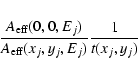
The background spectrum from the merged closed event file was obtained using the same method. The NXB is not vignetted; however, since the correction is applied to the total (CXB+NXB) spectrum from the merged sky event list, the same correction to the (pure NXB) spectrum, extracted from the same detector region, is required. This photon weighting method has the advantage of allowing for an exact correction of the vignetting effect, accounting for a non-uniform exposure map as well as for spatial variations in the NXB.

   
3.6 Renormalization of the NXB spectrum

A renormalization is needed to account for the different intensities of the NXB in the sky fields and in the closed observations due to the non-simultaneity of the measurement. To compute the renormalization factor, taking advantage of the very high statistic, we used the energy range 10-11.2 keV where no fluorescence lines (possibly having different time behaviour wrt. the continuum, see Appendix A) are present and where the expected CXB signal is negligible, being of order 0.2%. The ratio of the count rates in the total (CXB+NXB) and (pure NXB) spectra is computed and used as renormalization factor for the NXB spectrum. In Sect. 5.4 we will study the effects of the uncertainty in this operation.

   
3.7 Spectral analysis

The spectra from the merged sky fields were rebinned by a factor of 10 to obtain a good statistic in each energy channel after background subtraction. The adopted vignetting correction method requires the use of the on-axis redistribution matrices and effective area files. For each camera, we used an exposure-weighted effective area file computed as a linear combination of the MOS1/2 effective areas provided by the XMM-Newton Science Operation Centre for the different optical filters, the weights being the fractions of the total exposure time corresponding to each filter.

The 2-8 keV range was selected for the analysis. Lower energies were not used to avoid (i) contaminations by the soft galactic component of the CXB (emerging below $\sim$1 keV) and (ii) possible artefacts due to an imperfect subtraction of the bright Al-K and Si-K fluorescence lines (in the 1-2 keV range - see Appendix A). Above 8 keV the collected CXB signal is marginal.

The spectral analysis was performed within XSPEC v11.0. The spectral model was a simple absorbed power law. The interstellar absorption $N_{\rm H}$ was fixed to the exposure-weighted average of the values of the selected fields. We added to the model multiple Gaussian lines to account for possible differences in intensity of the brightest fluorescence lines (Cr, Mn, Fe in the 5-7 keV spectral range) in the sky and in the closed observations. Their energies and FWHM (which are constant across the detector plane, see Sect. A.2) were fixed to the values computed using the out FOV data (sky and closed observations yielded fully consistent results).

To minimize the correlation between the CXB spectral parameters (photon index and intensity), the normalization of the power law was evaluated at the barycentre of the selected energy range (see Ulrich & Molendi 1996), which in our case is found to lie at $\sim$3 keV. MOS1 and MOS2 data were studied both separately and in a symultaneous fit.

	Figure 3: The cosmic X-ray background spectrum in the 2-8 keV range is displayed, folded with the instrumental response. MOS1 data are represented in grey, MOS2 in black. The best fit model is overplotted. The lower panel shows the residuals in units of sigma.
Open with DEXTER

   
4 Results

The final dataset includes 42 sky fields for the MOS1 camera and 43 for the MOS2. The total exposure time is of $\sim$1.15 Ms per camera. The solid angle covered by the data, summing the contribution of each observation (accounting for the differences in field of view due to the readout mode or to the excision of the central target) is of $\sim$5.5 square degrees (34 different pointing directions) per camera. The closed data amount to $\sim$430 ks per camera.

The spectrum of the cosmic X-ray background as seen by the MOS instruments is shown in Fig. 3. We note that the CXB signal is very low if compared to the quiescent NXB, accounting for only $\sim$20% of the counts in the (vignetting-corrected) spectrum from the sky field merged dataset in the 2-8 keV range.

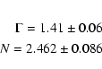
The two cameras yield fully consistent results within the statistical uncertainties (see Table 1). A symultaneous fit to the data ( $\chi^{2}_{\nu}=1.15$, 72 d.o.f.) yields a photon index of 1.41 $\pm$ 0.04 and a normalization of 2.647 $\pm$ 0.038 photons cm^-2 s^-1 sr^-1 keV^-1 at 3 keV (to be corrected for the stray light, i.e. the contribution to the collected flux due to photons coming from out-of-field angles). The quoted uncertainties are the statistical errors at the 90% confidence level for a single interesting parameter.

Table 1: Results of the spectral analysis on the CXB for the MOS cameras. The normalization is expressed in photons cm^-2 s^-1 sr^-1 keV^-1 at 3 keV (not corrected for the stray light contribution). The quoted uncertainties are purely statistical errors at the 90% confidence level for a single interesting parameter.

A careful study of the possible sources of errors led us to compute the overall uncertainty (systematics included) to be of 4% for the photon index and of 3.5% for the normalization. The details of the error analysis are presented in the next section.

After correcting for the stray light (see Sect. 5.6), the MOS results on the 2-8 keV CXB spectrum are:

$$\begin{eqnarray*}\Gamma = 1.41\pm0.06 \\ N = 2.462\pm0.086 \end{eqnarray*}$$

where the normalization N is expressed in photons cm^-2 s^-1 sr^-1 keV^-1 at 3 keV.

The resulting flux in the 2-10 keV energy range is of (2.24 $\pm$ 0.16) $\times$ 10^-11 erg cm^-2 s^-1 deg^-2. The error (90% confidence) includes also an extra 5% uncertainty as an estimate of the absolute flux calibration accuracy of the MOS cameras. To ease a comparison with previous works, the corresponding normalization at 1 keV is of $\sim$11.6 photons cm^-2 s^-1 sr^-1 keV^-1.

   
5 Analysis of errors

A very careful evaluation of the possible sources of error, including systematics, is of paramount importance in the measure of a faint source such as the CXB. In the following sections the quoted errors on the spectral parameters are at 90% confidence level for a single interesting parameter.

   
5.1 Effect of the use of different SAS versions

As stated in Sect. 3.1, in this work different SAS releases (namely v5.0, v5.3.0, 5.3.3) were used to perform the preliminary processing of the data. We processed $\sim$100 ks per camera of closed observations with the SAS v5.3.3 to be compared with the corresponding datasets in our compilation processed through SAS v5.0. The analysis and the extraction of the spectra were performed as described in Sect. 3. A linear fit to the ratio of the two spectra in the range 2-12 keV was found to be fully consistent with a constant equal to 1, the slope being statistically null. Nevertheless, as a further step we used the computed (90% confidence) limits on the slope to modify the final quiescent NXB spectrum (i.e. the one used in Sect. 4); such "distorted'' spectrum was used to study the CXB, running the second part of our pipeline. We obtained a variation of $\sim$2% in the best fit photon index value, and a variation of $\sim$1.5% in the normalization. Such values, comparable to the statistical uncertainties (see Sect. 4), represent a very conservative estimate (indeed, a worst case) of the possible systematics associated with the use of different SAS versions.

Figure 4: The best fit photon index of the CXB is plotted as a function of the selected GTI threshold (in units of sigma of the quiescent count rate distribution - see Sect. 3.2). Errors (at 90% confidence level for a single interesting parameter) include the uncertainty on the renormalization of the quiescent NXB spectrum. The adopted 3.3$\sigma$ threshold is marked by the vertical solid line. No significant variations in the CXB photon index are obtained as a result of different choices of the GTI threshold within the range $\sim$ $2.9{-}3.8\sigma$, marked by the dotted vertical lines.

Open with DEXTER

   
5.2 Effect of different thresholds for soft proton screening

We took advantage of our automated pipeline to study the effects of different prescriptions for the GTI filtering (see Sect. 3.2) directly on the best fit parameters of the CXB, simply running the whole pipeline several times, using different values for the GTI selection parameters. While different recipes to build the light curve are generally less efficient, we investigated the effects of a different choice for the count rate threshold. This is indeed a crucial problem. Lumb et al. (2002) reported a variation of the cosmic background spectral parameters as a results of different flare screenings, but they did not present any systematic study of this effect.

Figure 5: Same as Fig. 4, the best fit CXB normalization is shown. Units are photons cm-2 s-1 sr-1 keV-1 at 3 keV. The contributions from out-of-field scattered light have not been subtracted. Errors (at 90% confidence level for a single interesting parameter) include the uncertainty on the renormalization of the quiescent NXB spectrum. The adopted GTI threshold is marked by the vertical dashed line. It is evident that no significant variations are obtained as a result of small changes of the selected GTI threshold (within the range $\sim$ $2.9{-}3.8\sigma$, marked by the dotted vertical lines). See text for further details.

Open with DEXTER

The results for the photon index and the normalization of the CXB as a function of the threshold (in units of sigma from the average count rate) are shown in Figs. 4 and 5. It is evident that the selected 3.3$\sigma$ level represent an optimal threshold. Little changes in the adopted value (in both directions) have essentially no effects on the best fit CXB parameters. The choice of significantly lower values implies the rejection of positive random fluctuations from the good count rate, lowering the inferred normalization; conversely, the choice of significantly higher values implies the inclusion of a fraction of soft proton NXB which increase the derived CXB normalization. Within the "good'' range for the GTI threshold identified in this study ($\sim$ $2.9\sigma{-}3.8\sigma$), the variations of the photon index and normalization of the CXB spectrum are always smaller than the statistical uncertainties. We therefore consider any systematic error associated with the GTI thresholding to be negligible.

Figure 6: Best fit CXB photon index as a function of the maximum allowed ratio for the 8-12 keV surface brightness $\Sigma _{{\rm IN}}/\Sigma _{{\rm OUT}}$, a probe of the presence of residual soft proton NXB. The MOS1 case is shown (MOS2 is very similar). Errors (at 90% confidence level for a single interesting parameter) include the uncertainty on the renormalization of the quiescent NXB spectrum. No significant changes are obtained. The case of the CXB normalization is markedly different (see Fig. 7).

Open with DEXTER

Figure 7: Same as Fig. 6, the best fit CXB normalization (in units of photons cm-2 s-1 sr-1 keV-1 at 3 keV) is plotted here. The stray light correction have not been applied. Errors (at 90% confidence level for a single interesting parameter) include the uncertainty on the renormalization of the quiescent NXB spectrum. When dataset having large values of the ratio $\Sigma _{{\rm IN}}/\Sigma _{{\rm OUT}}$ are included, the normalization is systematically higher owing to the presence of a significant residual SP NXB component (see text). The adopted maximum allowed ratio ( $R_{{\rm MAX}}=1.3$) is marked by the vertical line. No significant changes are obtained within small changes of  $R_{{\rm MAX}}$. See Appendix B for further details.

Open with DEXTER

   
5.3 Effect of a different threshold for the residual soft proton NXB

As shown in Appendix B.2, the residual soft proton background may introduce a strong bias in the measure of the CXB spectral parameters. It is therefore very important to check if our recipe to define a good, non-contaminated dataset on the basis of the ratio of surface brightnesses  $\Sigma _{{\rm IN}}/\Sigma _{{\rm OUT}}$ (see Sect. 3.3 and Appendix B) is a possible source of systematics. We studied directly the variation of the CXB spectral parameters as a function of the threshold  $R_{{\rm max}}$ on the ratio  $\Sigma _{{\rm IN}}/\Sigma _{{\rm OUT}}$. For each selected value of  $R_{{\rm max}}$ (we explored the range $\sim$0.95-2.7), the datasets below the threshold were merged and the CXB spectrum extracted and analyzed running our automatic pipeline. The computed best fit CXB photon index and normalization are plotted as a function of the threshold  $R_{{\rm max}}$ in Figs. 6 and 7, respectively. While the value of the photon index does not change significantly as a function of  $R_{{\rm max}}$, in the case of the normalization a peculiar trend is seen and can be easily interpreted. When the threshold  $R_{{\rm max}}$ is high (>1.5), the contribution of the contaminated observations is important. Decreasing values of  $R_{{\rm max}}$ yield therefore a significant variation in the CXB normalization as a result of the rejection of an increasing number of bad observations. The trend disappears and the normalization become stable when the contaminated observations have been discarded. Further decreases of  $R_{{\rm max}}$ lead to the exclusion of good observations with positive fluctuations of the ratio  $\Sigma _{{\rm IN}}/\Sigma _{{\rm OUT}}$. The break occurs for  $R_{{\rm max}}$ $\sim$1.5. We assume conservatively $R_{{\rm max}}$ = 1.3 to define our final dataset to study the CXB. An inspection of Figs. 6 and 7 shows that for slightly different choices of  $R_{{\rm max}}$ in the "good'' range $\sim$1.0 $\div$ 1.4 the variations of the best fit CXB slope and normalization are small with respect to the statistical uncertainties. We conclude therefore that our approach for identifying and rejecting contaminated observations is robust and free from systematics.

We note in addition that a new break is observed in Fig. 7 for  $R_{{\rm max}} \sim$ 0.95. This occurs when the threshold  $R_{{\rm max}}$ is below the average value of the ratio  $\Sigma _{{\rm IN}}/\Sigma _{{\rm OUT}}$. In these cases, only dataset with a negative fluctuation of the ratio are included.

   
5.4 Effect of the NXB spectrum renormalization

As stated in Sect. 4, the NXB accounts for $\sim$80% of the counts in the 2-8 keV energy range for a blank sky observation. It is therefore evident that even small errors in the renormalization of the NXB spectrum can yield large effects on the inferred CXB spectrum. The uncertainty on the renormalization factor, computed using standard error propagation, is of 0.8% for both MOS1 and MOS2. This translates in an uncertainty of 2.1% in the best fit photon index for the CXB spectrum, and of 1.9% for the normalization.

   
5.5 Check of the vignetting curve calibration

The vignetting function of the X-ray telescopes is well calibrated (Lumb et al. 2002; Kirsch 2003); the main sources of uncertainty (currently under investigation by the calibration team) are a possible $\sim$1 arcmin offset of the optical axis from the nominal position and the azimuthal modulation induced by the Reflection Gratings Assemblies, installed on the light path of the X-ray telescopes having the MOS cameras at their primary foci. As a consequence, the absolute flux of a point source has an uncertainty of order $\leq$5%. Since in this work we use events extracted from almost all of the MOS field of view, the uncertainty on the collected flux induced by the two quoted effects should be much lower, since possible errors in the vignetting corrections across the FOV should partially compensate. Following Lumb et al. (2002), we therefore assume 1.5% as an estimate of the uncertainty on the effective areas.

As a consistency check, we have divided the FOV of the instrument into six regions lying at increasing off-axis angles from the nominal optical axis position, namely a central circle of 4 arcmin radius and 5 circular annuli of 2 arcmin width. We repeated the whole analysis for each region separately, computing independent values for the best fit spectral parameters of the CXB. In Figs. 8 and 9 we plotted the photon index and the normalization of the CXB as a function of the off-axis angle for the MOS1 camera; the MOS2 case is very similar. As expected, no systematic effects can be seen, the observed fluctuations are smaller than the statistical uncertainties.

A study of the vignetting curve calibration using slew data is currently in progress. A preliminary analysis of $\sim$180 ks of data showed hints of deviations from the nominal behaviour in agreement with the above quoted hypothesis of an offset of the aimpoint. The stray light component (see next section), possibly centrally peaked, may also play a role (Lumb, private communication).

Figure 8: Best fit CXB photon index as a function of the off-axis angle. Each point represents an independent measure obtained from the analysis of a selected portion of the detector plane (see text). Errors (at 90% confidence level for a single interesting parameter) include the uncertainty on the renormalization of the quiescent NXB spectrum. The MOS1 case is shown (MOS2 is very similar). The constant trend is a result of the correct vignetting function calibration.

Open with DEXTER

Figure 9: Same as Fig. 8, the case of the CXB normalization is presented here. Units are photons cm-2 s-1 sr-1 at 3 keV. The corrections for the light coming from out-of-field angles have not been applied. Errors (at 90% confidence level for a single interesting parameter) include the uncertainty on the renormalization of the quiescent NXB spectrum. The variations are always smaller than the uncertainty, confirming the overall correctness of the vignetting curve calibration.

Open with DEXTER

   
5.6 Stray light

At the time of writing, no updates in the evaluation of the contribution to the collected flux from photons gathered from out-of-field angles have been published by the calibration team. We therefore assume the estimate by Lumb et al. (2002): an out-of-field scattered flux of order 7% of the good focused in-field signal, with an associated systematic uncertainty of 2%.

The main contribution to the stray light is due to sources within 0.4-1.4 degrees from the optical axis (Lumb et al. 2002). As a further check, we have used the available data from past and current X-ray mission to search for very bright sources lying in the quoted annular region for each of the pointings. We found only one relatively bright source at the $\sim$3 $\times$ 10^-11 erg cm^-2 s^-1level in the 2-8 keV energy range. A few (5) other sources were found, with fluxes of the order of a few 10^-12 erg cm^-2 s^-1. According to the efficiency of the X-ray baffle quoted by Lumb et al. (2002), these should not represent a matter of concern for the evaluation of the CXB normalization.

Table 2: Results of the spectral analysis on the CXB for the MOS cameras. Only single pixel events (PATTERN 0) have been used. The normalization is expressed in photons cm^-2 s^-1 sr^-1 keV^-1 at 3 keV (not corrected for the stray light contribution). The quoted uncertainties are purely statistical errors at the 90% confidence level for a single interesting parameter.

5.7 Effect of event PATTERN selection

For a consistency check, we repeated the spectral analysis for the case of PATTERN 0 events only (i.e. single pixel events, see XMM-Newton Users' Handbook). The results are reported in Table 2, where the quoted errors are pure statistical uncertainties at the 90% confidence level for a single interesting parameter.

When the uncertainty associated to the renormalization of the quiescent NXB spectrum ($\sim$2% for both the photon index and the normalization, see Sect. 5.4) is taken into account, the results from the PATTERN 0-12 data (Sect. 4) and from PATTERN 0 events only are found to be in good agreement. We therefore assume any systematic effect associated with the event PATTERN selection to be negligible.

5.8 Effect of the internal fluorescence line modeling

The fluorescence line component of the quiescent NXB varies strongly across the detector plane (see Sect. A.2). To account for this effect, we extract the source (sky fields) and background (closed) spectra from the same detector region. Residual differences in the line intensity are due to time variation of the fluorescence NXB (sky fields and closed observations are not symultaneous), possibly different with respect to the continuum NXB variation which is corrected by the closed spectrum renormalization. To solve the problem we have included multiple Gaussian lines in the CXB spectral model (see Sect. 3.7).

To assess the possible effect of such correction on the CXB best fit parameters, we have repeated the spectral analysis removing the Gaussian lines. In this case, the fit to the data is found to be somewhat worse ( $\chi^2_{\nu}=1.28$, 79 d.o.f.), owing to higher residuals in correspondence of the line energies. The best fit normalization is found to be in full agreement (within less than 0.1%) with the value quoted in Sect. 4, while the photon index is consistent within $\leq$2% ($\leq$$1 \sigma$statistical uncertainty).

We note that when the correction is applied, any systematic effect on the CXB spectral parameters should be smaller than the above quoted differences, and therefore negligible with respect to the pure statistical errors.

   
5.9 Absolute flux calibration

We can evaluate the uncertainty affecting absolute flux measurements with EPIC/MOS on the basis of the results of the cross-calibration with other satellites. Kirsch (2003) and Molendi & Sembay (2003) reported a comparison of the spectral results on suitable calibration sources studied with different instruments. The agreement on the measured fluxes in the 1-10 keV range is very good, within a few %, with a standard deviation of order 5%. We assume 5% as a conservative estimate of the uncertainty on the absolute flux calibration of EPIC.

   
6 Discussion

Our measurement of the intensity of the Cosmic X-ray Background has been plotted in Fig. 10 (adapted from Moretti et al. 2003), together with previous determinations. To be conservative, to identify the most probable range of sky surface brightness constrained by our data, we have used an estimate of the accuracy of the cross-calibration in absolute flux among different recent instruments (see Sect. 5.9) as a measure of the absolute flux calibration uncertainty of EPIC.

Our results are in full agreement with the BeppoSAX LECS/MECS analysis of Vecchi et al. (1999) and with the study of Lumb et al. (2002) using XMM-Newton EPIC/MOS data. The ASCA GIS measure of Kushino et al. (2002) is marginally consistent with ours, while the HEAO-1 value (Marshall et al. 1980) is significantly lower.

As discussed by Barcons et al. (2000), part of the dispersion of the different measurement can be ascribed to cosmic variance. The above authors estimated that differences up to $\sim$10% in the CXB intensity are expected when the solid angle is of order 1 square degree. They concluded therefore that systematic errors and cross-calibration differences among different instruments must be present.

Figure 10: CXB intensity measurements. The flux in the 2-10 keV band is represented as a function of the epoch of the experiment. The plot is an update of Fig. 3 of Moretti et al. (2003) including the results of the present work. From left to right the CXB values are from Marshall et al. (1980) with HEAO-1 data; McCammon et al. (1983) with a rocket measurement; Gendreau et al. (1995) with ASCA SIS data; Miyaji et al. (1998) with ASCA GIS; Ueda et al. (1999) with ASCA GIS and SIS; Vecchi et al. (1999) with BeppoSAX LECS/MECS; Lumb et al. (2002) with XMM-Newton EPIC/MOS; Kushino et al. (2002) with ASCA GIS. Finally, the hollow star mark our own CXB measurement with the EPIC MOS cameras onboard XMM-Newton. All the uncertainties are at 1$\sigma$ level. The horizontal dotted lines mark the range of CXB intensity constrained by our measurement after including an extra 3.2% uncertainty (1$\sigma$ confidence level, rescaled from the 5% uncertainty quoted in the text, which corresponds to 90% confidence level) on the absolute flux calibration of the EPIC cameras (it is indeed a measure of the cross-calibration accuracy among different instruments). Such range represents the most robust estimate of the true absolute sky surface brightness in the 2-8 keV band.

Open with DEXTER

The HEAO-1 measurement, performed on $\sim$10⁴ square degrees, is very robust for solid angle coverage. However, all of the subsequent measurements yielded systematically higher values, casting at least some doubts on the absolute flux calibration of the HEAO-1 instruments. We note that a recent reanalysis of the HEAO-1 data (Gruber et al. 1999), as pointed out by Gilli (2003), showed differences of order 10% among different detectors in the overlapping energy ranges.

Two new measurements have been published since the analysis of Barcons et al. (2000). Lumb et al. (2002) used a combination of 8 XMM-Newton EPIC/MOS pointings covering $\sim$1.2 square degrees. Their approach for the instrumental background subtraction (based on a model of the out FOV spectrum) is markedly different from ours and therefore their determination is to be considered largely independent from the measurement presented in this work. The ASCA/GIS study of Kushino et al. (2002) was performed over a large solid angle ($\sim$50 square degrees) to minimize the effects of cosmic variance. However, the large stray light component ($\sim$40% of the collected flux) affecting ASCA represents a severe limit to the absolute flux measurement of the CXB, which they estimated to be uncertain at the $\sim$10% level.

In our analysis, we used a compilation of sky pointings covering $\sim$5.5 square degrees. The effects of cosmic variance (roughly scaling as $\Omega^{-1/2}$) on our measure of the CXB intensity should be rather small, being of the same order of the overall quoted uncertainty ($\sim$4%). Our measurement, performed with the well-calibrated EPIC/MOS instrument, relies on a very robust characterization and subtraction of the instrumental background; possible sources of systematics were carefully studied and their impact on the determination of the CXB spectrum was evaluated. In conclusion, these considerations, coupled to the excellent agreement of our findings with the results of two of the most recent investigations, lead us to believe that the measurements of the CXB intensity have finally converged to a well constrained value, significantly higher than the former result from HEAO-1 data, assumed more than 20 years ago as a reference.

It is very interesting to compare our new measurement of the CXB intensity with the source number counts derived from the recent deep X-ray observations. Moretti et al. (2003) have built a log N/log S function using a very large source compilation, including the results from six different surveys, both pencil-beam and wide-field, performed with ROSAT, Chandra and XMM-Newton. We assume here their results for the integrated flux of the 2-10 keV source counts down to the sensitivity limit of the 1 Ms Chandra Deep Fields ($\sim$1.7 $\times$ 10^-16 erg cm^-2 s^-1). Our measurement of the CXB intensity, $F_{{\rm CXB}}$ = (2.24 $\pm$ 0.10) $\times$ 10^-11 erg cm^-2 s^-1 deg^-1 ($1 \sigma$ error, including the absolute flux uncertainty), implies that 80 ⁺⁷_-6% of the cosmic X-ray background has been resolved into discrete sources in the 2-10 keV band. Even extrapolating the log N/log S down to fluxes of $\sim$10^-17 erg cm^-2 s^-1 (a factor of 10 below the detection limit of the deep surveys) the integrated flux would rise only to $\sim$84% of the CXB (due to the slow growth of the faint branch of the log N/log S), not consistent with its total value. A new class of faint sources (possibly heavily absorbed AGNs, or star-forming galaxies, see Moretti et al. 2003 and references therein) could emerge at fluxes of a few 10^-16 erg cm^-2 s^-1, steepening the log N/log S and accounting for the remaining part of unresolved CXB. Some contribution to the CXB could also be due to truly diffuse emission.

The analysis of the deepest 2 Ms Chandra Deep Field North and of the XMM deep pointing to the Lockman Hole and of their associated multiwavelength follow-up campaigns, will shed light on the issue. On the basis of a well constrained value for the CXB intensity, the new observations will further our understanding of the CXB nature.

Note added in proof: After the present paper had been accepted for publication, a measurement of the CXB spectrum with the PCA insrument onboard RXTE was published by Revnivtsev et al. (2003).

Acknowledgements

We are grateful to all the members of the EPIC collaboration for their work and their support. We thank Alberto Moretti and Sergio Campana for providing their compilation of past CXB measurements. We thank the referee, David Lumb, for his suggestions. ADL acknowledges ASI for a fellowship.

References

 
• Baldi, A., Molendi, S., Comastri, A., et al. 2002, ApJ, 564, 190 In the text NASA ADS  
• Barcons, X., Mateos, S., & Ceballos, M. T. 2000, MNRAS, 316, L13 In the text NASA ADS  
• Brandt, W. N., Alexander, D. M., Hornschemeier, A. E., et al. 2001, AJ, 122, 2810 In the text NASA ADS  
• De Luca, A., & Molendi, S. 2002, in New Visions of the X-Ray Universe in the XMM-Newton and Chandra Era (Noordwijk: ESA), ESA SP-488, in press [arXiv:astro-ph/0202480] In the text  
• Fabian, A. C., & Barcons, X. 1992, ARA&A, 30, 429 In the text NASA ADS  
• Gendreau, K., Mushotzky, R., Fabian, A. C., et al. 1995, PASJ, 47, L5 In the text NASA ADS  
• Giacconi, R., Gursky, H., Paolini, F. R., & Rossi, B. B. 1962, Phys. Rev. Lett., 9, 439 In the text NASA ADS  
• Giacconi, R., Bechtold, J., Branduardi, G., et al. 1979, ApJ, 234, L1 In the text NASA ADS  
• Giacconi, R., Zirm, A., Wang, J., et al. 2002, ApJS, 139, 369 In the text NASA ADS  
• Gilli, R., Salvati, M., & Hasinger, G. 2001, A&A, 366, 407 In the text NASA ADS  
• Gilli, R. 2003, to appear in New X-ray Results from Clusters of Galaxies and Black Holes, ed. C. Done, E. M. Puchnarewicz, & M. J. Ward, Advances in Space Research [arXiv: astro-ph/0303115] In the text  
• Hasinger, G., Altieri, B., Arnaud, M., et al. 2001, A&A, 365, L45 In the text NASA ADS  
• Katayama, H., Takahashi, I., Ikebe, Y., et al. 2002, in New Visions of the X-Ray Universe in the XMM-Newton and Chandra Era (Noordwijk: ESA), ESA SP-488, in press [arXiv:astro-ph/0201440] In the text  
• Kirsch, M. (on behalf of the EPIC collaboration) 2003, EPIC Calibration issues in progress, Document XMM-SOC-CAL-TN-0018-2-1 (EPIC Status of Calibration and Data Analysis), XMM Science Operation Centre, Villafranca del Castillo, available from In the text http://xmm.vilspa.esa.es/external/xmm_sw_cal/calib/index.shtml  
• Kushino, A., Ishisaki, Y., Morita, U., et al. 2002, PASJ, 54, 327 In the text NASA ADS  
• Lumb, D. H., Warwick, R. S., Page, M., & De Luca, A., 2002, A&A, 389, 93 In the text NASA ADS  
• Markevitch, M., Bautz, M. W., Biller, B., et al. 2003, ApJ, 583, 70 In the text NASA ADS  
• Marshall, F. E., Bolt, E. A., Holt, S. S., et al. 1980, ApJ, 235, 4 In the text NASA ADS  
• Mather, J. C., Cheng, E. S., Eplee, R. E., et al. 1990, ApJ, 354, L37 In the text NASA ADS  
• McCammon, D., Burrows, D. N., Sanders, W. T., & Kraushaar, W. L. 1983, ApJ, 269, 107 In the text NASA ADS  
• Miyaji, T., Ishisaki, Y., Ogasaka, Y., et al. 1998, A&A, 334, L13 In the text NASA ADS  
• Molendi, S., & Sembay, S. 2003, EPIC Calibration issues in progress, Document XMM-SOC-CAL-TN-0036-1-0, XMM Science Operation Centre, Villafranca del Castillo, available from In the text http://xmm.vilspa.esa.es/external/xmm_sw_cal/calib/index.shtml  
• Moretti, A., Campana, S., Lazzati, D., & Tagliaferri, G. 2003, ApJ, 588, 696 In the text NASA ADS  
• Revnivtsev, M., Gilfanov, M., Sunyaev, R., Jahoda, K., & Markwardt, C. 2003, A&A, 411, 329 In the text NASA ADS  
• Setti, G., & Woltjer, L. 1989, A&A, 224, L21 In the text NASA ADS  
• Strüder, L., Briel, U., Dennerl, K., et al. 2001, A&A, 365, L18 In the text NASA ADS  
• Turner, M. J. L., Abbey, A., Arnaud, M., et al. 2001, A&A, 365, L27 In the text NASA ADS  
• Ueda, Y., Takahashi, T., Inoue, H., et al. 1999, ApJ, 518, 656 In the text NASA ADS  
• Ulrich-Demoulin, M.-H., & Molendi, S. 1996, ApJ, 457, 77 In the text NASA ADS  
• Vecchi, A., Molendi, S., Guainazzi, M., Fiore, F., & Parmar, A. N. 1999, A&A, 349, L73 In the text NASA ADS  
• Vercellone, S. 2000, Document EPIC-MCT-TN-006 (Flat-field analysis for Orsay FM3 MOS campaign - Part II: maps & trends), IFC-CNR, Milan, Italy  
• XMM-Newton Users' Handbook 2003, Issue 2.1, ed. M. Ehle et al., XMM Science Operation Centre, Villafranca del Castillo, available from http://xmm.vilspa.esa.es/external/xmm_user_support/documentation/uhb/index.html  
• Zimmermann, U., Boese, G., Becker, W., et al. 1998, EXSAS User's Guide, MPE Report, ROSAT Scientific Data Center In the text

  
Online Material

   
Appendix A: An independent measure of the quiescent NXB spectrum

The quiescent NXB component due to the interaction of high-energy particles with the detectors and the other structures of the telescopes/cameras bodies can be studied in two ways: (i) considering the out FOV regions of the detectors and (ii) using the closed observations. In both cases, the collected signal is purely cosmic-ray induced, with no contributions from X-ray photons or soft protons.

To measure the CXB spectrum, out FOV regions offer the advantage of a NXB measurement simultaneous with the CXB observation. A disadvantage is represented by possible spatial variations of the NXB spectrum across the plane of the detectors: in such case, the out FOV spectrum would not be an adequate representation of the NXB present in an observation of the sky. Closed observations allow for the extraction of the NXB spectrum from the same detector region where the CXB is collected, but the two measurements are not simultaneous. Time variations of the NXB spectrum may render closed observations useless for our study. These problems will be addressed in the following sections.

A.1 Spectral characterization of the quiescent NXB

The spectrum extracted from the merged closed dataset, selecting the in FOV region, is presented in Fig. A.1. The total exposure time is of $\sim$430 ks. In the same plot we show the spectra extracted from the out FOV region for the sky fields merged dataset (total exposure $\sim$1.15 Ms) and the closed dataset. The 2-12 keV continuum is well represented by a flat power law not convolved with the telescope collecting areas and CCD quantum efficiencies, with a photon index of $\sim$0.2. Several bright emission lines are seen, due to fluorescence emission from materials of the telescope and the camera bodies. The strongest are the Al-K line from the shielding of the cameras and the Si-K line from the back substrate of the CCD chips (its intensity is much smaller in the out FOV spectrum); additional lines from Cr, Mn, Fe, Zn, Au are also visible. For further details see Lumb et al. (2002).

   
A.2 Spatial distribution of the quiescent NXB

It is known that the quiescent NXB changes slightly across the field of view (e.g. Lumb et al. In the text 2002). The strongest spatial variations are seen in correspondence with the internal fluorescence emission lines. Lumb et al. (2002) showed the peculiar, non-uniform distribution of the Al-K (strongly suppressed near the edges of CCD#1) and of the Si-K (strongly brighter near the edges of CCD#1) emission (see their Figs. 2 and 3), due to shadowing effects as a consequence of the non-planar disposition of the CCD chips.

An inspection of Fig. A.1 immediately shows the different relative strength of the fluorescence lines in the quiescent in FOV and out FOV NXB. Apart from the above mentioned Al-K and Si-K cases, it is evident that the Au emission (most probably associated with the gold coated readout flexible circuits) is much stronger in the out FOV spectrum. In particular, the prominent structure at $\sim$2.15 keV in the out FOV spectrum is virtually absent in FOV.

Figure A.1: Quiescent NXB spectrum for the MOS1 camera. From top to bottom: data from closed observations (black), in FOV region; from the sky merged dataset (red), out FOV region; from closed obs.(green), out FOV region. The closed out FOV spectrum has been rescaled by a factor of 3 to ease its visibility; no renormalization was performed on the other spectra. Total exposure time is of $\sim$430 ks for the closed spectra, $\sim$1.15 Ms for the sky data. The labels identify the strongest internal fluorescence lines. Significant differences in the fluorescence lines intensities are evident between the in FOV and the out FOV spectra.

Figure A.2: Ratio between the spectra extracted from the out FOV region for the sky merged dataset and for the closed dataset. Data are from the MOS1 camera; the MOS2 case is very similar. A linear fit to the range 2-12 keV is fully consistent with a constant.

To investigate the possible presence of spatial variations in the continuum, we have studied the closed NXB on each CCD detector separately. The spectra were fitted in the 2-12 keV range with a model consisting of a power law with the addition of multiple Gaussians to reproduce the fluorescence lines, not convolved with the telescope areas and the CCD quantum efficiencies. We found, as expected, strong variations in the line intensities (their energies and width are found to be stable); marginally significant variations in the photon index were also seen.

The observed variations of the quiescent NXB across the FOV strongly suggest that it is better to extract the NXB and the source spectra from the same region of the detector. This is particularly important in the case of the faint CXB, whose signal is lower than the NXB over the whole 2-8 keV energy range.

To assess whether the closed observations are indeed representative of the actual quiescent NXB affecting a typical sky field observation, we compared the closed spectrum extracted from the out FOV region with the corresponding out FOV spectrum from the merged sky dataset. Apart from a multiplicative factor required to match the intensities (due to the non-simultaneity of the measurements), we did not find significant differences either in the continuum shape (the best fit photon indexes were almost indistinguishable) or in the line components. In Fig. A.2 we show the ratio between the two spectra. The results of a linear fit to the ratio in the range 2-12 keV are fully consistent with a constant.

   
A.3 Temporal behaviour of the quiescent NXB

Non-simultaneous measurements of the NXB can be used to study the CXB only if the NXB spectrum is stable in time. As a first step, we studied the secular variation of the NXB surface brightness in different energy ranges. As a typical example, we show in Fig. A.3 the light curves in the 8-12 keV band for the out FOV regions of the sky observations and for the closed observations (the in FOV region was selected in this case).

The main results are:

• the large majority of the observations follow a smooth secular trend: the surface brightness decreases by 30% from revolution 50 to revolution 100, reaches a minimum around revolution 150 and thereafter slowly increases;

• the secular trend and the absolute surface brightness values for the normally behaving cases are almost equal for the sky field data out FOV and the closed observations;

• The points deviating from the general trend correspond to observations performed under high radiation conditions. For instance, the closed observation of revolution 329 was taken during an intense solar flare;

• during high radiation periods, the intensity of the NXB can be more than an order of magnitude higher than average;

• the scatter around the good behaviour is of order 15% for the sky observations, while it is much higher for the closed observations, since the latter are often performed at the beginning/end of the visibility window of the orbit, closer to the perigee, where the flux of particles (from the radiation belts) is generally more intense than in the higher part of the satellite orbit.

The light curves in other energy bands are very similar and are not reported here. What is important to the aim of the present study (as well as for the study of faint diffuse sources) is to assess the stability of the quiescent NXB spectral shape. In Fig. A.4 we plot the surface brightness in the band 1.4-1.6 keV (dominated by the Al-K internal fluorescence line) versus the 2.5-5 keV band (continuum emission only) for the closed observations. It is evident that, although a definite correlation is present, the scatter of the points is rather high. A very similar effect is seen comparing the 0.5-1.2 keV band with the 2.5-5 keV; on the contrary, the correlation between the 2.5-5 keV and the 8-12 keV bands is much better (see Fig. A.5).

Figure A.3: Secular variation of the surface brightness (units of counts cm-2 s-1) in the 8-12 keV range for MOS1 (red points) and MOS2 (black points): out FOV regions in sky fields observations (empty squares) and in FOV region in closed observation (filled squares). A smooth trend having a broad minimum around revolution $\sim$150 is seen; a high scattering, due to different particle radiation conditions, is also evident.

This suggests that the spectral shape may change in time, the fluorescence lines having a time behaviour quite different from the high energy continuum. A similar result was reported for the pn camera by Katayama et al. (2002). A poor correlation is also seen between the low energy and the high energy parts of the continuum, while the 2-12 keV band presents a rather coherent behaviour. These results have important implications for the study of faint diffuse sources when an independent measurement of the background spectrum is needed: a simple renormalization of the quiescent NXB using the high energy range (e.g. 8-12 keV) count rate could lead to systematic errors in both the continuum (low energy wrt. high energy) and the lines.

Figure A.4: The correlation between the surface brightness (units of counts cm-2 s-1) in the 1.4-1.6 keV range (dominated by the internal Al-K fluorescence line - see Fig. A.1) and the surface brightness in the range 2.5-5 keV (continuum). Data are for closed observations; MOS1 red and MOS2 black. A rather high scatter is evident.

Figure A.5: Same as Fig. A.4; the surface brightness (units of counts cm-2 s-1) in the energy ranges (2.5-5 keV) and (8-12 keV) show a better correlation.

We investigated in more detail the dependence of the NXB spectral shape on the intensity of the high-energy particle flux. We divided the sample of the closed observations in two parts, a "high intensity'' dataset and a "low intensity'' dataset (respectively, above and below a 8-12 keV surface brightness of 0.007 cts cm^-2 s^-1, see Fig. A.3). We then extracted the spectra from the in FOV region. We show in Fig. A.6 the ratio of the two spectra. As expected from the previous analysis, differences are observed in the low energy part of the continuum and in correspondence of the brightest fluorescence lines; however, the most interesting result is that the ratio above 2 keV is constant. We tried a linear fit to the data in the 2-12 keV range; the slope was found to be statistically null.

Figure A.6: Ratio of the spectra from the "high intensity'' and "low intensity'' samples of closed observations (see text) for the MOS1 camera. The MOS2 case is very similar. Although deviations are seen in correspondence of the fluorescence lines, the overall shape in the 2-12 keV range is clearly constant: the shape of the quiescent NXB spectrum is stable in spite of high variations in the flux of high energy particles.

This demonstrates that the NXB continuum spectral shape in this energy range does not depend on the intensity of the impinging flux of cosmic rays; no significant changes are seen even in presence of very large variations in intensity. It is therefore possible to use non-simultaneous measures of the quiescent NXB spectrum for the study of the 2-8 keV CXB. The only caveat is to compute a renormalization factor in order to match the intensity of the NXB component present in the two dataset.

A.4 Conclusions

The results of the study of the quiescent NXB can be summarized as follows.

• The ratio between the closed and the sky field (out FOV) spectra shows that closed observations give a correct representation of the quiescent NXB present in a typical observation of the sky.

• The spatial analysis revealed strong variations in the fluorescence line component across the detector plane, as well as hints for variations in the continuum. A NXB spectrum extracted from the same detector region where the CXB is collected would therefore be preferable.

• The temporal analysis demonstrated that variations up to a factor of 10 in intensity may occur during high radiation periods. The spectral shape may change in time; in particular, the low energy (0.5-1.2 keV) and high energy (>2 keV) continuum variations are poorly correlated; the same is true for continuum and fluorescence line component. In any case, the spectral shape above 2 keV is very stable, at least for the continuum.

The use of the closed observations is more appropriate to get an indepenent measurement of the quiescent NXB required to study the CXB.

   
Appendix B: Any residual soft proton contamination?

A very important step to get a robust measure of the faint CXB spectrum is to investigate the presence of a residual component of soft proton NXB in the GTI-filtered event lists, as a consequence of a steady flux of particles impinging the detectors and/or of other peculiar conditions of low-energy particle irradiation. A soft proton contamination could indeed affect the study of faint diffuse sources; so far, no systematic investigations of this problem were published (but see De Luca & Molendi 2002 for a preliminary report).

In the case of the ACIS instrument onboard Chandra, rather similar to XMM-EPIC in both the orbit and the detector technology, Markevitch et al. (2003) reported that the spectrum of the dark Moon is consistent with the spectrum collected when the CCDs are in the stowed position (outside the field of view) and therefore the steady flux of low energy particles can be as low as zero. In any case, the low statistic in the dark Moon spectra, coupled to the small number of observations, prevented the authors from drawing definitive conclusions. However, Markevitch et al. (2003) showed that "long flares'', having a very low time variability along an observation, may occasionally occur, affecting the spectral study of faint diffuse sources. The higher collecting area suggests a priori that in similar conditions the flow of gathered particles could be higher (and therefore its impact on science more important) for XMM/EPIC than for Chandra/ACIS.

In the next sections we will present a simple diagnostic to reveal and quantify the residual soft proton component affecting an observation; we will also study its impact on the measure of the CXB spectrum.

Figure B.1: The correlation between the 8-12 keV surface brightness (counts cm-2 s-1) in FOV and out FOV is shown for the sky fields observations. Red and black points represent MOS1 and MOS2 observations, respectively. A high scatter is clearly evident.

Figure B.2: Same of Fig. B.1 for the case of the closed observations. The correlation is much better.

Figure B.3: The ratio of the 8-12 keV surface brightness ( in FOV)/( out FOV) is plotted as a function of the surface brightness in FOV (counts cm-2 s-1). Data are from sky fields observations, red points correspond to MOS1 and black points to MOS2. A definite correlation is absolutely evident.

Figure B.4: The ratio $\Sigma _{{\rm IN}}/\Sigma _{{\rm OUT}}$ (8-12 keV) is plotted here as a function of  $\Sigma _{{\rm OUT}}$ (counts cm-2 s-1). No correlation can be seen in this case, markedly different from the result presented in Fig. B.3.

Figure B.5: The light curve of this observation looks "typical'' at first glance, with intense soft proton flares superposed on a quiescent count rate. However it is found that the quiescent count rate is much higher than the value expected for a typical blank sky field (marked by the dashed line) and shows a slow modulation. The whole observation is affected by a "long flare'' of low-energy particles; the analysis of the 8-12 keV surface brightness after GTI screening clearly indicates an anomalous ratio  $\Sigma _{{\rm IN}}/\Sigma _{{\rm OUT}}$.

Figure B.6: Light curve of an observation badly affected by soft proton flares during all of its duration. The expected count rate for a typical sky field is marked by the dashed line. The automated GTI filtering algorithm used in our study cannot properly work in such conditions (see text).

Figure B.7: The ratio of the 8-12 keV surface brightness $\Sigma _{{\rm IN}}/\Sigma _{{\rm OUT}}$ is plotted as a function of  $\Sigma _{{\rm IN}}$ (counts cm-2 s-1) for the sky fields (blue points) and for the closed observations (green points). A linear fit to the two distributions is overplotted. It is evident that the sky fields observations show higher values of  $\Sigma _{{\rm IN}}/\Sigma _{{\rm OUT}}$ even in the less contaminated cases.

   
B.1 A diagnostic to reveal soft proton contamination

The basic idea to identify the residual low energy particle background is to look for its signature in terms of a non-uniform distribution of the count rates across the plane of the detectors, due to the focusing of the particles by the telescope optics. We studied therefore the surface brightness in the regions inside and outside the field of view: any residual soft proton component should be visible only in FOV. We selected the high energy band (8-12 keV), excluding the central CCD in order to minimize the presence of genuine cosmic X-rays in the count rate in FOV.

As a first step, we plotted the surface brightness in FOV ( $\Sigma _{{\rm IN}}$) versus the surface brightness out FOV ( $\Sigma _{{\rm OUT}}$). This is shown in Fig. B.1. A clear correlation is present; however, a rather high scatter of the points is evident. The same plot obtained for the case of the closed observations shows a much better correlation (see Fig. B.2).

As a second step, we studied whether the scatter in Fig. B.1 can be ascribed to an anomalous flux in FOV. This is absolutely clear from Fig. B.3, where we have plotted the ratio of the surface brightness  $\Sigma _{{\rm IN}}/\Sigma _{{\rm OUT}}$ versus the surface brightness  $\Sigma _{{\rm IN}}$. Such a clear correlation is not seen at all in the plot of  $\Sigma _{{\rm IN}}/\Sigma _{{\rm OUT}}$ vs. $\Sigma _{{\rm OUT}}$ presented in Fig. B.4.

It is thus evident that in some observation the NXB surface brightness inside the field of view is higher than outside. From Fig. B.3, we can see that the most pathological cases can show a quiescent NXB intensity up to 300% higher than average. We note that such anomalous count rates are to be entirely ascribed to an enhanced NXB component, since the signal expected from the CXB in the selected energy range and off-axis angle is of order of $\sim$0.5% of the overall count rate, and no bright sources are present in our selected fields.

We inspected the light curves of the most deviating observations. Two phenomenologies, as expected, were observed. First, a very smooth light curve, with an average "quiescent'' count rate significantly higher than expected for a typical blank sky field, and slow time variability along the observation duration (see Fig. B.5). These could be the cases of "long flares'' of soft protons, affecting the whole observation and showing little or no time variability, similar to what occasionally observed by Markevitch et al. (2003) in the Chandra case. Second, conversely, a highly variable light curve with almost no quiescent time intervals (Fig. B.6). In both cases, as stated in Sect. 3.3, our automated GTI filtering algorithm cannot be efficient since all of the observing time is affected by a flux of low energy particles.

In Fig. B.7 the same plot as in Fig. B.3 is presented; data from closed observations have been overplotted. It is evident that for closed observations the ratio of the surface brightness  $\Sigma _{{\rm IN}}/\Sigma _{{\rm OUT}}$ remains constant under all of the observed low energy particle irradiation conditions. The results of a linear fit to the two distributions are also interesting: the ratio $\Sigma _{{\rm IN}}/\Sigma _{{\rm OUT}}$is found to be lower for the closed observations. This is true also for the sample of sky fields observations which are less affected by the residual soft proton component. In correspondence of the average value of the surface brightness in FOV for these observations ( $\Sigma_{{\rm IN}}\sim0.0065$ cts cm^-2 s^-1 in 8-12 keV), the ratio $\Sigma _{{\rm IN}}/\Sigma _{{\rm OUT}}$ for the sky fields is higher by $\sim$10%. Although this difference is seen at a low level of significance (<3$\sigma$), this may be a hint for the presence of an irreducible flow of low energy particles reaching the detectors during all science observations.

Figure B.8: Spectra extracted from the sky fields observations having different values of the ratio R of surface brightness  $\Sigma _{{\rm IN}}/\Sigma _{{\rm OUT}}$: R < 1.05 (green - dataset "a''), 1.05 < R < 1.30 (red - dataset "b''), R > 1.30 (black - dataset "c'').

Figure B.9: Best fit CXB parameters computed from the three independent dataset corresponding to different values of  $\Sigma _{{\rm IN}}/\Sigma _{{\rm OUT}}$ (see text and Fig. B.8 for the color code. The normalization is in photons cm-2 s-1 sr-1 keV-1 at 3 keV. The stray light contribution have not been subtracted. Errors (at 90% confidence level for a single interesting parameter) include the uncertainty on the renormalization of the quiescent NXB spectrum. The normalization and the photon index computed for the dataset  c) are uncompatible with the values for dataset  a) and  b), which are found, conversely, to be in good agreement.

   
B.2 Impact on science of the residual soft proton component

In the previous section we showed that a residual component of soft proton background is sometimes (possibly always) present within the field of view. It is very important to assess whether such NXB component can affect the scientific analysis of faint diffuse sources, and, if this is the case, to define a recipe to recover reasonable results from contaminated observations.

To this aim we divided our sample of observations in different independent subsets, corresponding to different levels of contamination, the ratio R of surface brightnesses  $\Sigma _{{\rm IN}}/\Sigma _{{\rm OUT}}$ being a measure of the residual SP NXB level. We selected three ranges of R: <1.05 (negligible contamination - dataset "a''), $1.05\div1.30$ (low contamination - dataset "b''), >1.30 (significant contamination - dataset "c''). In each of the three cases, we applied the algorithm described in Sect.  3 (in particular, the steps corresponding to Sect. 3.4 $\div$ 3.7) to extract and analyze the CXB spectrum, obtaining three independent determinations of the best fit CXB parameters. The three total (CXB+quiescent NXB) spectra are plotted together in Fig. B.8; the corresponding best fitting normalizations and photon indexes are shown in Fig. B.9.

It is evident that the parameters inferred from the most contaminated dataset (c) are totally incompatible with the results of dataset (a) and (b). The slope of the CXB spectrum is found to be flatter than expected, while the best fit normalization is higher by more than 100% (more than 15$\sigma$ for a single interesting parameter) with respect to dataset (a). The results from datasets (a) and (b), on the contrary, are found to be in good agreement in both the slope and the normalization. Thus, the simple recipe described in Sect. 3 works well up to values of $\sim$1.3 for the ratio R, i.e. in presence of a low contaminating SP component.

As a further step we studied the spectral shape of the contaminating background component. The differences in count rate among the three datasets can be ascribed, in principle, to three causes: (i) presence of residual SP NXB, (ii) variations of the quiescent NXB, (iii) cosmic variance, due to the discrete nature of the CXB. In order to get the spectrum of the "pure'' residual SP NXB, it is necessary to remove the variability due to the other causes.

As shown in Appendix A, the variation in the quiescent NXB level from observation to observation may be significant; however, merging several observations (at least six, as in dataset (c) for the MOS2), the variance should be lower. We evaluated the actual level of the quiescent NXB in each of the three datasets using the corresponding out FOV spectrum. An ad hoc renormalized closed spectrum was then subtracted from each of the three spectra to remove the quiescent NXB component.

Cosmic variance should not play an important role in the comparison of the three spectra. As discussed by Barcons et al. (2000), the expected variance in the CXB intensity is of order 10% on a solid angle $\Omega$ of 1 square degree, scaling roughly as $\Omega^{-{\frac{1}{2}}}$. The minimum solid angle is covered by dataset (c) ($\sim$1.5 square degree). Since the CXB signal accounts only for $\sim$10% of the 2-12 keV count rate, we see that only differences <1% can be due to cosmic variance.

Any difference among the three (quiescent NXB subtracted) spectra can therefore be ascribed to the residual SP NXB. Assuming the level of such NXB component to be 0 in dataset (a), we extracted the pure residual SP NXB spectrum affecting datasets (b) and (c) by means of the simple subtraction of spectrum (a).

The NXB affecting dataset (c) is found to have a spectrum well described by a power law having photon index of $\sim$-0.05 and an exponential cutoff at $\sim$5 keV, not convolved with the telescope effective areas and the CCD quantum efficiencies. This is the typical spectral shape of a particle-induced background component. Markevitch et al. (2002) reported a very similar result for the "flare'' spectra affecting Chandra ACIS observations.

The good statistics allowed to repeat the analysis for each single observation belonging to dataset (c). The results clearly showed that the spectrum of the contaminating component is not stable. The significant differences in the spectral shape can be equally well reproduced, within the statistical uncertainty, with variations in the photon index or in the exponential cutoff position. We note that cosmic variance, even on a solid angle as small as the single observation field of view, could account only for a minor part of the observed variations. It is very likely that the spectrum of the residual NXB component depend on the energy distribution of the impinging particles; in any case, more detailed analyses are beyond the scope of this work.

Turning now to dataset (b), we find that the spectrum of the anomalous NXB, within the limits of a lower statistics, can be well described by the same model used for the case (c).

B.3 Conclusions

The results on the study of the residual soft proton background can be summarized as follows:

• As a result of peculiar low-energy particle radiation conditions, a significant soft proton NXB component can survive after GTI screening.
• A study of the ratio of surface brightness  $\Sigma _{{\rm IN}}/\Sigma _{{\rm OUT}}$ in the high energy range (8-12 keV) can easily reveal the presence of such residual NXB.
• The spectral shape is a flat power law with an exponential cutoff, not convolved with the telescope effective areas and the CCD quantum efficiencies, typical of particle background.
• The intensity can be highly variable. Increases in the NXB count rate up to 300% can occur.
• The spectral slope is highly variable and unpredictable, being possibly dependent on the energy distribution of the impinging particles.
• Spectral study of extended sources may be heavily affected.
• When the intensity of the residual soft proton NXB is low (up to 30% higher than average) a simple renormalization of the quiescent background spectrum yields acceptable results owing to the very flat spectral shape of the low-level soft proton spectrum. The NXB level in the observation under exam must be evaluated within the FOV (better at large off-axis angles), using the high energy range (better excluding fluorescence lines, if the statistics is good).
• There are hints for the presence of an irreducible flow of low-energy particles always reaching the detectors. Its impact on the analysis of the CXB is negligible.