A&A 419, 425-437 (2004)
DOI: 10.1051/0004-6361:20034566
Numerical study of the cosmological velocity field as a
function of density
A. Domínguez1,2 - A. L. Melott3
1 - Max-Planck-Institut für Metallforschung,
Heisenbergstr. 3, 70569 Stuttgart, Germany
2 -
Theoretische Physik, Ludwig-Maximilians-Universität,
Theresienstr. 37, 80333 München, Germany
3 -
Department of Physics and Astronomy, University of Kansas, Lawrence, Kansas 66045, USA
Received 23 October 2003 / Accepted 5 February 2004
Abstract
We report on a new study of the velocity distribution in
N-body simulations.
We investigate the center-of-mass and internal kinetic energies of
coarsening cells as a function of time, cell size and cell mass. By
using self-similar cosmological models, we are able
to derive theoretical predictions for comparison and
to assess
the influence of finite-size and resolution effects.
The most interesting
result is the discovery of a polytropic-like relationship between
the average velocity dispersion (internal kinetic energy) and the mass density in an intermediate
range of densities,
 .
The exponent
.
The exponent  measures the deviations from the virial prediction,
 .
For self-similar models, depends only on
the spectral index of the initial power spectrum. We also study CDM models and confirm a
previous result that the same polytropic-like dependence exists,
with a time and coarsening length dependent .
The dependence
.
For self-similar models, depends only on
the spectral index of the initial power spectrum. We also study CDM models and confirm a
previous result that the same polytropic-like dependence exists,
with a time and coarsening length dependent .
The dependence
 is an important input for a
recently proposed theoretical model of cosmological structure
formation which improves over the standard dust model (pressureless fluid) by regularizing
the density singularities.
is an important input for a
recently proposed theoretical model of cosmological structure
formation which improves over the standard dust model (pressureless fluid) by regularizing
the density singularities.
Key words: gravitation - methods: N-body simulations - cosmology: large-scale structure of Universe
The use of N-body simulations has proved a useful tool in the
investigation of both the cosmological structure formation and the
evolution by self-gravity. The main interest has been
concentrated on properties of the spatial distribution of matter (mass
correlations, void distribution, morphological features...),
while the kinetic properties have received comparatively little
attention, without doubt due to the larger difficulties to obtain
reliable kinetic measurements from real data with which to compare (Watkins et al. 2002).
The kinetic measurements addressed till
now with N-body simulations have pertained the quasilinear velocity field
(see e.g. the reviews by Dekel 1994 and Bernardeau et al. 2002; an application closely related to the present work is Seto & Sugiyama 2001),
the pairwise relative velocity (Peebles 1980; for recent
applications, see e.g. Feldman et al. 2003; Strauss et al. 1998),
and the velocity dispersion of halos (e.g. Knebe & Müller 1999 in connection with the present work).
Our work
addresses the center-of-mass velocity of coarsening cells ( macroscopic kinetic energy), as well as the velocity dispersion of
the particles inside the cell (internal kinetic energy). The
coarsening cells are randomly centered and of variable size (probing
both the linear and the nonlinear regimes); in this way our analysis
does not suffer the arbitrariness intrinsic to the definition of
clusters and halos (Klypin & Holtzmann 1997, and references therein),
and essentially all the simulation particles are employed in the
determination of the quantities.
We are aware of two works where a similar analysis of
N-body simulations has been performed (Nagamine et al. 2001; Kepner et al. 1997),
motivated differently than ours.
The connection to our work is explained in Sect. 5 in detail.
The present study focuses on the dependence of the cell kinetic
energies on the cell mass density. The main motivation is the
application to models of cosmological structure formation by
self-gravity. The most widely used theoretical model is the dust model
(pressureless fluid) (Padmanabhan 1995; Peebles 1980), which has been studied
intensively (see e.g. the reviews Bernardeau et al. 2002; Sahni & Coles 1995) but has the
shortcoming of producing singularities. Some recent works
(Domínguez 2000; Maartens et al. 1999; Buchert et al. 1999; Adler & Buchert 1999; Buchert & Domínguez 1998; Tatekawa et al. 2002; Morita & Tatekawa 2001; Domínguez 2002) have
proposed a novel approach. One of its features is the ability to
derive adhesion-like models (Kofman & Shandarin 1988; Kofman et al. 1992; Gurbatov et al. 1989; Melott et al. 1994; Sathyaprakash et al. 1995),
and to offer a possible explanation of the physical origin for the
"adhesive'' behavior which regularizes the mass density singularities
of the dust model. In these improved models, the internal kinetic
energy brings about the "adhesive'' behavior provided it can be
approximated as a function of density and/or the gradients of the
velocity field.
Another goal of this work is to confirm the results by
Domínguez (1999,2003), where a polytropic-like dependence between
internal kinetic energy and mass density is found in AP3M simulations of CDM models. We indeed corroborate this finding in PM simulations of CDM models and also of self-similar models. The latter
are particularly amenable to a theoretical analysis and allow the
identification of the influence of finite-size and resolution effects
in the measurements. We conclude that the polytropic-like dependence
is unlikely to be an artifact of the simulations.
The paper is organized as follows: in Sect. 2 we work
out the theoretical predictions for the density dependence of the
macroscopic and internal kinetic energies.
In Sect. 3 we describe the simulations and the method
how we measure the kinetic energies. In Sect. 4 we
present the results of the analysis. Section 5
contains a discussion of the results and the conclusions.
2 Theoretical background
Let a(t) denote the cosmological expansion factor, m the mass of a particle,
and
 and
and
 the comoving position and
peculiar velocity, respectively, of the
the comoving position and
peculiar velocity, respectively, of the  th particle.
 is a (normalized) smoothing window. Then, given a comoving
smoothing scale L, the coarse-grained mass density field, velocity
field and density of internal peculiar kinetic energy are
defined respectively as follows:
is a (normalized) smoothing window. Then, given a comoving
smoothing scale L, the coarse-grained mass density field, velocity
field and density of internal peculiar kinetic energy are
defined respectively as follows:
![\begin{displaymath}
\varrho {\vec u} ({\vec x}, t; L) = \frac{m}{[a(t) L]^3}
...
...t) ~
W \left({{\vec x}-{\vec x}_\alpha (t) \over L} \right),
\end{displaymath}](/articles/aa/full/2004/20/aa0566/img47.gif) |
(1) |
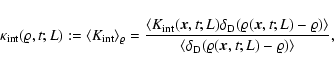
The density of macroscopic![[*]](/icons/foot_motif.gif) peculiar kinetic energy is defined as
peculiar kinetic energy is defined as
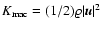 ,
so that one can write
,
so that one can write
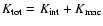 ,
where
,
where
 is the density of total peculiar kinetic energy: this is given by the same expression
as
is the density of total peculiar kinetic energy: this is given by the same expression
as
 above but dropping
  .
Whether
.
Whether
 or
dominates the contribution to
means respectively
that the particle velocities
are controlled by the
center-of-mass motion of the coarsening cell as a whole or by
"internal'' motions within the cell (the ratio
or
dominates the contribution to
means respectively
that the particle velocities
are controlled by the
center-of-mass motion of the coarsening cell as a whole or by
"internal'' motions within the cell (the ratio
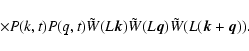
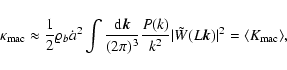
 was introduced as the cosmic Mach number by Ostriker & Suto 1990). Indeed,
is a much
better probe of the dynamics at the small scales than
,
because in the latter there can be extensive cancellations in the
vectorial sum defining .
was introduced as the cosmic Mach number by Ostriker & Suto 1990). Indeed,
is a much
better probe of the dynamics at the small scales than
,
because in the latter there can be extensive cancellations in the
vectorial sum defining .
The
purpose of the present study is the
relationship between
and the field  .
Our main interest is
the density dependence of
.
Our main interest is
the density dependence of
 ,
that is, the average of
conditioned to a given value
of the coarse-grained mass density,
,
that is, the average of
conditioned to a given value
of the coarse-grained mass density,
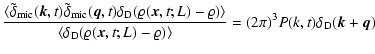
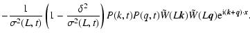
 |
(2) |
where
 denotes ensemble average, which by
translational invariance must be
denotes ensemble average, which by
translational invariance must be  -independent, and
 is Dirac's delta function. In the same
way is defined the conditioned average
is Dirac's delta function. In the same
way is defined the conditioned average
 .
Since
.
Since
 receives contributions from
the highly non-linear regime, the density dependence cannot be
computed analytically in general. Nevertheless, a lot can be learned
by way of suitable approximations, whose validity will be checked by
comparing with simulations.
receives contributions from
the highly non-linear regime, the density dependence cannot be
computed analytically in general. Nevertheless, a lot can be learned
by way of suitable approximations, whose validity will be checked by
comparing with simulations.
To simplify the theoretical discussion, we consider a self-similar
cosmological model: an Einstein-de Sitter background and an initial
Gaussian distributed density field with power spectrum
 ,
with the bounds n>-3 (so that density
fluctuations do not receive a divergent contribution from
,
with the bounds n>-3 (so that density
fluctuations do not receive a divergent contribution from
 )
and n<4 (imposed by the unavoidable graininess due
to the point particles) (Padmanabhan 1995; Peebles 1980). The conclusions should
apply qualitatively unaltered to a more realistic case. Let
)
and n<4 (imposed by the unavoidable graininess due
to the point particles) (Padmanabhan 1995; Peebles 1980). The conclusions should
apply qualitatively unaltered to a more realistic case. Let
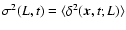 denote the variance
of the density contrast smoothed on the scale L (
denote the variance
of the density contrast smoothed on the scale L (
 is the density contrast, with
 the background density),
(A tilde will denote a Fourier transform.)
A (comoving) scale of nonlinearity,
 ,
is defined by the
condition
,
is defined by the
condition
In the self-similar model, the physical properties which do not depend
on the short and large distance cutoffs of P(k)exhibit a simple scaling behavior (Padmanabhan 1995; Peebles 1980). The only physically
relevant parameters on which they can depend are
 (through the cosmological background),
 (through the
initial conditions), and the gravitational constant G (through the
dynamics); self-similarity means that the time t0 is arbitrary.
Thus, in combination with dimensional analysis, it is shown that
(through the
initial conditions), and the gravitational constant G (through the
dynamics); self-similarity means that the time t0 is arbitrary.
Thus, in combination with dimensional analysis, it is shown that
 is a function of the single quantity
 ;
in the linear
regime,
;
in the linear
regime,
 ,
one has
,
one has
 .
Similarly,
.
Similarly,
 can be written in the following
suggestive form:
can be written in the following
suggestive form:
 |
(3) |
Here  is a dimensionless function of its dimensionless
arguments, and
is a dimensionless function of its dimensionless
arguments, and
 is of the order of the
Hubble-flow kinetic energy in balls of (comoving) radius
is of the order of the
Hubble-flow kinetic energy in balls of (comoving) radius
 .
The unconditioned averages
.
The unconditioned averages
 and
and
 follow the same scaling but
without the
follow the same scaling but
without the  -dependence. Deviations from this scaling
behavior would mean a dependence on extra variables, e.g., on short or
large distance cutoffs in P(k) or in the dynamics (as occurs with,
e.g., numerical simulations).
-dependence. Deviations from this scaling
behavior would mean a dependence on extra variables, e.g., on short or
large distance cutoffs in P(k) or in the dynamics (as occurs with,
e.g., numerical simulations).
The task now is to characterize the functions
 .
Let
.
Let  and R denote the short and the
large distance cutoffs, respectively,
so that we take
and R denote the short and the
large distance cutoffs, respectively,
so that we take
 .
Roughly speaking, we can
say that
.
Roughly speaking, we can
say that
 is determined by the motion at scales between L and R, whereas
is dominated by the motion at scales between
and L.
is determined by the motion at scales between L and R, whereas
is dominated by the motion at scales between
and L.
![\begin{figure}
\par\resizebox{8.8cm}{!}{\includegraphics[clip]{figures/0566f1.eps}}
\end{figure}](/articles/aa/full/2004/20/aa0566/Timg86.gif) |
Figure 1:
Sketch representing the relative contribution of the different
length scales to
and
.
The scales , R and
are intrinsic to the system, the movable length L is the observation resolution. |
| Open with DEXTER |
The hierarchical, bottom-up scenario exhibits a monotonically growing
length scale,
,
which
is roughly proportional to the size of the largest collapsed clusters at time t.
The bottom-up growth of structure by self-gravity can be sketched in
the following picture:
particles get trapped in clusters so that (i) the evolution above the
cluster scale is dominantly ruled by the motion of each cluster as a
whole (="effective particles'') in the gravitational field of the
other clusters, and (ii) the evolution below the cluster scale is
driven mainly by the scales  cluster size. This means a
dynamical decoupling between scales above and below the
cluster size,
(this idea has been explored by
Domínguez (2000, 2002),
in
order to improve the models of structure formation), and implies that
the short-distance cutoff
is irrelevant. Depending on which
of the two motions, (i) or (ii), contributes mostly to the particle
velocity, there arise several possibilities (see Fig. 1):
cluster size. This means a
dynamical decoupling between scales above and below the
cluster size,
(this idea has been explored by
Domínguez (2000, 2002),
in
order to improve the models of structure formation), and implies that
the short-distance cutoff
is irrelevant. Depending on which
of the two motions, (i) or (ii), contributes mostly to the particle
velocity, there arise several possibilities (see Fig. 1):
- if -3<n<-1, it will be argued that the largest scales dominate.
Thus,
should be determined by the scales R and
by
the scales L;
- if -1<n<4, the scales around
provide the prevalent
contribution because
is irrelevant and there is no other
privileged scale between
and
.
We can distinguish
in turn two cases:
- linear regime,
 :
the value of
is
mainly set by scales
:
the value of
is
mainly set by scales  ,
and that of
by scales
,
and that of
by scales
 ;
;
- nonlinear regime,
 :
now
is dominated by
scales
,
and
by scales .
:
now
is dominated by
scales
,
and
by scales .
This description will be now elaborated in somewhat more detail.
Case I: -3<n<-1. There is so much power initially at the large
scales, that the contribution of the linear modes (
 )
to
the variance of the macroscopic velocity diverges if n<-1:
)
to
the variance of the macroscopic velocity diverges if n<-1:
Hence, both
and the particle velocities
will be mainly determined by the modes around the largest available
scale, the infrared (IR) cutoff R.
For the macroscopic kinetic energy we then estimate
 |
(4) |
 |
(5) |
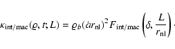
For the internal kinetic energy, it proves useful to consider
separately the linear and nonlinear regimes:
- Linear regime,
.
Our hypothesis is that the main
contribution to
comes from scales L, so that we can
employ the linear solutions to the gravitational instability to
evaluate Eqs. (1). The calculations are collected
in the Appendix; the final result reads
![\begin{displaymath}
{\kappa}_{\rm int}= \langle K_{\rm int} \rangle \left[ 1 + B \left(
1 - \frac{\delta^2}{\sigma^2(L)} \right) \right]\cdot
\end{displaymath}](/articles/aa/full/2004/20/aa0566/img98.gif) |
(6) |
In this expression,
 is the unconditioned
average internal peculiar kinetic energy in the linear
approximation, Eq. (A.2), B is a dimensionless
negative numerical coefficient, Eq. (A.3). Both
and B are IR-convergent because the R-dependence cancels from the difference
is the unconditioned
average internal peculiar kinetic energy in the linear
approximation, Eq. (A.2), B is a dimensionless
negative numerical coefficient, Eq. (A.3). Both
and B are IR-convergent because the R-dependence cancels from the difference
 ,
so that Eq. (3) holds. Indeed, we derive the scaling
behavior
,
so that Eq. (3) holds. Indeed, we derive the scaling
behavior
 |
(7) |
- Nonlinear regime,
.
In high-density coarsening cells,
 ,
the Hubble flow is negligible and peculiar
velocities are approximately equal to the physical velocities.
Assuming stationarity, the conditioned differences
,
the Hubble flow is negligible and peculiar
velocities are approximately equal to the physical velocities.
Assuming stationarity, the conditioned differences
 can be expected to be given
by local virialization on scales ,
so that
can be expected to be given
by local virialization on scales ,
so that
 |
(8) |
The opposite limit of low density,
 ,
requires a
model for the expansion of voids. The simplest model would set
,
requires a
model for the expansion of voids. The simplest model would set
 typically, with
 quantifying the void expansion speed. Then
 |
(9) |
predicting a low internal kinetic energy.
To compute the unconditioned average
,
it
must be noticed that, although the internal kinetic energy of
high-density cells is very large, the number of low-density cells is
much larger, and it is not clear which of the two competing effects
dominates. If one would assume that the main contribution comes from
high-density cells, then
Eq. (8) would yield
 |
(10) |
Case II: -1<n<4. The linear modes do not lead to divergences
and the velocities are now determined mainly by the scale
.
- Linear regime,
.
Now the linear solution states
that the smoothed velocity
will be determined by scales L, i.e., the smallest scales it probes, and thus one obtains
 |
(11) |
On the other hand, our hypothesis is that the particle velocities
are controlled by scales
.
Hence, we
write the estimate
assuming that the scales
are rather insensitive to the
small density fluctuations at the scale
.
Then
 |
(12) |
- Nonlinear regime,
.
The conditioned difference
 is controlled
by the local dynamics on scales L like in the previous case,
and expressions (8-10) are valid now
too. The motion of the coarsening cells as a whole, and thus
is controlled
by the local dynamics on scales L like in the previous case,
and expressions (8-10) are valid now
too. The motion of the coarsening cells as a whole, and thus
 ,
is however assumed to be
determined by the large scales
,
so that
,
is however assumed to be
determined by the large scales
,
so that
 |
(13) |
in analogy to Eqs. (12).
3 Simulation and analysis method
The simulations of the self-similar models are described in full
detail elsewhere (Melott & Shandarin 1993). They consist of a cubic box (periodic
boundary conditions) of comoving sidelength R containing
N=1283 particles.
The dynamical evolution was computed using a PM algorithm on a grid
with Nyquist wavenumber
 .
The background cosmological
expansion followed the Einstein-de Sitter solution and the initial
conditions were generated by using the Zel'dovich approximation for a
Gaussian random field with a scale-invariant power spectrum
.
The background cosmological
expansion followed the Einstein-de Sitter solution and the initial
conditions were generated by using the Zel'dovich approximation for a
Gaussian random field with a scale-invariant power spectrum
 .
In the present work, the values n=-2, 0, +1 were considered
and the data were studied at three different times,
corresponding to a scale of nonlinearity
.
In the present work, the values n=-2, 0, +1 were considered
and the data were studied at three different times,
corresponding to a scale of nonlinearity
 ,
,
 ,
and
,
and
 ,
respectively. In each case
four independent realizations of the initial conditions were evolved.
,
respectively. In each case
four independent realizations of the initial conditions were evolved.
Two CDM models were also addressed with a PM algorithm: flat CDM
(
 ,
,
 ,
,
 ), and
open CDM (
), and
open CDM (
 ,
,
). Each simulation contained N=2563, and for each model two different box-sizes were considered, R=128 Mpc and R=512 Mpc.
,
,
). Each simulation contained N=2563, and for each model two different box-sizes were considered, R=128 Mpc and R=512 Mpc.
Starting from the coordinates
 provided by the simulation, the definitions (1) were applied with a cubic top-hat window,
 |
(14) |
where
 is the step function. The coarsening was
implemented efficiently by covering the simulation box with a cubic
grid; in order to probe a minimum of 2048 coarsening cells, the grid
was shifted randomly, when needed. It was checked that the results are
insensitive to the use of a spherical top-hat window instead. A
comparison with the use of a Gaussian window was also carried out. We
observed a difference only for the case n=+1 at the earliest time,
,
because then
is the step function. The coarsening was
implemented efficiently by covering the simulation box with a cubic
grid; in order to probe a minimum of 2048 coarsening cells, the grid
was shifted randomly, when needed. It was checked that the results are
insensitive to the use of a spherical top-hat window instead. A
comparison with the use of a Gaussian window was also carried out. We
observed a difference only for the case n=+1 at the earliest time,
,
because then  diverges for a top-hat window
(in the simulation, the artificial point-particle discreteness regularizes the
singularity). Hence, for this single case we disregarded the use of the cubic
top-hat window as unphysical and used instead a Gaussian window (which
is computationally much more costly).
diverges for a top-hat window
(in the simulation, the artificial point-particle discreteness regularizes the
singularity). Hence, for this single case we disregarded the use of the cubic
top-hat window as unphysical and used instead a Gaussian window (which
is computationally much more costly).
The explored values of the coarsening length L were equally
separated in a logarithmic scale and they ranged from a maximum (R/5) down to a minimum 
 ,
where
,
where
 is the average interparticle distance.
This results in scatter plots "kinetic energy vs. density''. To
compute the constrained average (2), the data for the
kinetic energy
were binned into 40 subintervals according to the value of the density ;
bins containing less than 10 data points were disregarded.
It was checked that the conclusions are robust against the amount of
binning by varying the number of bins.
The constrained average was identified with the mean of each bin.
The amount of scatter about this (global) mean is represented in the
plots by scatter bars, which extend between the mean of those
kinetic energies above the global mean, and the mean of
those kinetic energies below the global mean. We find that
this method represents the scatter of the data in the log-plots more
faithfully than the estimation through the variance.
is the average interparticle distance.
This results in scatter plots "kinetic energy vs. density''. To
compute the constrained average (2), the data for the
kinetic energy
were binned into 40 subintervals according to the value of the density ;
bins containing less than 10 data points were disregarded.
It was checked that the conclusions are robust against the amount of
binning by varying the number of bins.
The constrained average was identified with the mean of each bin.
The amount of scatter about this (global) mean is represented in the
plots by scatter bars, which extend between the mean of those
kinetic energies above the global mean, and the mean of
those kinetic energies below the global mean. We find that
this method represents the scatter of the data in the log-plots more
faithfully than the estimation through the variance.
We checked the algorithm in various ways. It was applied to an ideal
gas simulation: the results for the dependence of
on
the density agreed with the ideal gas equation of state. Another check
was to restrict the coarsening procedure to a subvolume of the
simulation box (1/64 of the total volume) for some sample cases.
As expected, we find that the data are somewhat noisier
because of the reduced number of particles, but the conclusions remain
the same.
4 Results
There are some general remarks which hold for all the subsections to follow.
First, the small length scale  enters in the results via
mass-resolution and force-resolution effects: the first effect refers to
the presence of a minimum non-vanishing mass - that of a single
particle.
This affects the computation of the unconstrained averages
enters in the results via
mass-resolution and force-resolution effects: the first effect refers to
the presence of a minimum non-vanishing mass - that of a single
particle.
This affects the computation of the unconstrained averages
 due to undersampling of the cells with a mass
smaller than this minimum, which also sets a lower bound on the value
of the density at a given fixed L when computing the constrained
averages,
,
.
In particular, it renders all results
concerning the nonlinear regime (
due to undersampling of the cells with a mass
smaller than this minimum, which also sets a lower bound on the value
of the density at a given fixed L when computing the constrained
averages,
,
.
In particular, it renders all results
concerning the nonlinear regime (
 )
at the earliest probed
time (
)
rather unreliable, since then
)
at the earliest probed
time (
)
rather unreliable, since then
 .
The second effect, force resolution, implies that the
relative force over two particles decreases when they are closer than
the mesh spacing of the PM algorithm, ,
and the velocity
dispersion below this scale does not grow as much as it would if
.
The second effect, force resolution, implies that the
relative force over two particles decreases when they are closer than
the mesh spacing of the PM algorithm, ,
and the velocity
dispersion below this scale does not grow as much as it would if
 .
All in all, these two effects tend to artificially
reduce the value of the kinetic energy, in particular of
,
being more sensitive to the small scales. The theoretical
discussion in Sect. 2 suggests this effect to be
particularly noticeable when n>-1 and at the earliest times, as indeed will
be observed.
.
All in all, these two effects tend to artificially
reduce the value of the kinetic energy, in particular of
,
being more sensitive to the small scales. The theoretical
discussion in Sect. 2 suggests this effect to be
particularly noticeable when n>-1 and at the earliest times, as indeed will
be observed.
Second, the influence of the "cosmic variance'', i.e., of the
fluctuations in measured quantities from one realization to another,
is the strongest when n=-2. For clarity, however, we will show in
the plots the results of a single realization, since the other ones
yield
almost identical results.
For reference purposes, Fig. 2 shows the measurements of
 .
The results collapse well on a single function of
.
The results collapse well on a single function of
 .
At the earliest time and the smallest lengths, one can
observe the beginning of the crossover to the Poissonian behavior,
.
At the earliest time and the smallest lengths, one can
observe the beginning of the crossover to the Poissonian behavior,
 ,
induced by the small-scale discreteness.
At large L, one recovers the linear scaling,
,
induced by the small-scale discreteness.
At large L, one recovers the linear scaling,
 ;
due to finite-size effects, the case n=-2 exhibits a
slight departure away from this dependence.
;
due to finite-size effects, the case n=-2 exhibits a
slight departure away from this dependence.
![\begin{figure}
\par\resizebox{8.8cm}{!}{\includegraphics[clip]{figures/0566f2a.e...
...r\resizebox{8.8cm}{!}{\includegraphics[clip]{figures/0566f2c.eps}}
\end{figure}](/articles/aa/full/2004/20/aa0566/Timg140.gif) |
Figure 2:
Abscissa:
 .
Ordinate: .
Ordinate:
 at the
three probed times. Solid line: expected functional dependence in
the linear regime,
at the
three probed times. Solid line: expected functional dependence in
the linear regime,
 . .
|
| Open with DEXTER |
The average
is the kinetic equivalent of .
In Fig. 3, we observe that the data for
do not follow at all the scaling
behavior (3) when n=-2. As explained in
Sect. 2, this is due to finite-size effects: we have
checked that the data follow instead the dependence (5).
The data for the other two cases, n=0,+1 on the contrary, obey the
expected scaling, Eq. (11) when
,
and
Eq. (13) when
.
A major departure in
the three cases is observed at the earliest time (
)
in the
nonlinear regime (
)
due to the undersampling problem mentioned above.
This was confirmed by artificially removing from the estimate of the
averages those cells with less than a given number of particles, yielding
the same behavior in
as detected in the
plots.
As remarked in Sect. 2, the average
is more sensitive to the small-scale dynamics than
or
are. This average also suffers
the same undersampling problem as
.
But
the resolution effects are somewhat larger and prevent the data from
following the scaling (3) perfectly. One can recognize
a tendency for these effects to become less relevant in time, and to
be more important for larger values of the spectral index n, in
agreement with the theoretical discussion.
![\begin{figure}
\par\resizebox{8.6cm}{!}{\includegraphics[clip]{figures/0566f3a.e...
... \resizebox{8.6cm}{!}{\includegraphics[clip]{figures/0566f3c.eps}}
\end{figure}](/articles/aa/full/2004/20/aa0566/Timg143.gif) |
Figure 3:
Abscissa:
.
Ordinate:
![$\log[\langle K \rangle
/ \varrho_b (\dot{a} r_{\rm nl})^2]$](/articles/aa/full/2004/20/aa0566/img141.gif) at the three probed times:
the lower points in each plot correspond to
;
the upper points represent
at the three probed times:
the lower points in each plot correspond to
;
the upper points represent
 .
The solid line is proportional to .
The solid line is proportional to
 ,
Eqs. (7), (10), (11). ,
Eqs. (7), (10), (11). |
| Open with DEXTER |
We first checked if the measured
followed the
self-similar scaling relationship (3). The conclusions
are almost the same as derived above with the unconstrained averages
:
follows self-similarity very
well (except if n=-2), while
follows it a bit less well. The
important difference is that departures from self-similarity are
(sometimes substantially) smaller than in
,
see Fig. 4. The reason is that
suffer the undersampling problem due to finite
mass-resolution only in the small-
end of each curve or at the earliest time. When the
number of particles in the cell is large enough, force-resolution is
likely the main effect and it does not appear to spoil self-similarity so much.
![\begin{figure}
\par\resizebox{8.6cm}{!}{\includegraphics[clip]{figures/0566f4a.e...
...\resizebox{8.6cm}{!}{\includegraphics[clip]{figures/0566f4b.eps}}
\end{figure}](/articles/aa/full/2004/20/aa0566/Timg146.gif) |
Figure 4:
Abscissa:
 .
Ordinate: .
Ordinate:
![$\log[{\kappa}_{\rm int}/\varrho_b (\dot{a}
r_{\rm nl})^2]$](/articles/aa/full/2004/20/aa0566/img145.gif) .
The plots are arbitrarily shifted in horizontal
direction for clarity. From left to right, .
The plots are arbitrarily shifted in horizontal
direction for clarity. From left to right,
 .
When self-similarity holds,
Eq. (3), curves corresponding to the same ratio
fall on top of each other. .
When self-similarity holds,
Eq. (3), curves corresponding to the same ratio
fall on top of each other. |
| Open with DEXTER |
Figure 5 shows the function
 at the different
times and coarsening lengths probed for the spectral index n=-2. The
scaling Eq. (4) is obeyed well at all times, although we
find small fluctuations around the linear
dependence between realizations. This is due to
the strong dependence on the IR cutoff. It is also responsible for the
lack of collapse of the three plots on a single function, the deviations
following indeed the law
at the different
times and coarsening lengths probed for the spectral index n=-2. The
scaling Eq. (4) is obeyed well at all times, although we
find small fluctuations around the linear
dependence between realizations. This is due to
the strong dependence on the IR cutoff. It is also responsible for the
lack of collapse of the three plots on a single function, the deviations
following indeed the law
 of the factor in
Eq. (4).
The slight deviations around
of the factor in
Eq. (4).
The slight deviations around  ,
most noticeable at the
earliest time, correspond to the largest values of L and are
likely due to finite-size effects too.
,
most noticeable at the
earliest time, correspond to the largest values of L and are
likely due to finite-size effects too.
![\begin{figure}
\par\resizebox{8.4cm}{!}{\includegraphics[clip]{figures/0566f5.eps}}
\end{figure}](/articles/aa/full/2004/20/aa0566/Timg151.gif) |
Figure 5:
Abscissa:
.
Ordinate:
![$\log[{\kappa}_{\rm mac}/ \varrho_b
(\dot{a} r_{\rm nl})^2]$](/articles/aa/full/2004/20/aa0566/img150.gif) .
Solid line: theoretical functional
dependence, Eq. (4). All the probed coarsening lengths,
at the three probed times (increasing from top to bottom) are
plotted. The scatter bars are barely dependent on time, coarsening
length and density; for clarity, they are shown only at the
earliest time. .
Solid line: theoretical functional
dependence, Eq. (4). All the probed coarsening lengths,
at the three probed times (increasing from top to bottom) are
plotted. The scatter bars are barely dependent on time, coarsening
length and density; for clarity, they are shown only at the
earliest time. |
| Open with DEXTER |
Figure 6 shows
in the linear regime when n=0,+1. The behavior (11) is obeyed very well within
the scatter bars; in the case n=0, a systematic trend away from the
expected data collapse is observed.
Figure 7 corresponds to the nonlinear regime. The
theoretical scaling Eq. (13) is also very well
followed within scatter bars. For the largest values of L considered
in the plot, a slight tendency is noticeable away from the theoretical
dependence, which is more obvious for n=+1.
Figure 8 shows
 for n=-2 in the linear
regime. Deviations from the theoretical prediction,
Eq. (6) with
and Bcomputed with Eqs. (A.2), (A.3),
are noticeable. The probable reason for
the discrepancy is that the linear regime is not really being probed:
one can observe a large asymmetry
for n=-2 in the linear
regime. Deviations from the theoretical prediction,
Eq. (6) with
and Bcomputed with Eqs. (A.2), (A.3),
are noticeable. The probable reason for
the discrepancy is that the linear regime is not really being probed:
one can observe a large asymmetry
 in the
plot, in contradiction with a centered Gaussian distribution
for .
(That deviations from Gaussianity are indeed important has
been checked by estimating the probability distribution of from the simulations.) The most linear case we probe for n=-2(corresponding to
and L=R/5) yields
in the
plot, in contradiction with a centered Gaussian distribution
for .
(That deviations from Gaussianity are indeed important has
been checked by estimating the probability distribution of from the simulations.) The most linear case we probe for n=-2(corresponding to
and L=R/5) yields
 ,
which satisfies the asymptotic condition
,
which satisfies the asymptotic condition
 only marginally. Thus, the ultimate origin of the problem is the IR cutoff imposed by the simulation box which limits the maximum value of L.
![\begin{figure}
\par\resizebox{8.5cm}{!}{\includegraphics[clip]{figures/0566f6a.e...
...\resizebox{8.5cm}{!}{\includegraphics[clip]{figures/0566f6b.eps}}
\end{figure}](/articles/aa/full/2004/20/aa0566/Timg157.gif) |
Figure 6:
Abscissa:  .
Ordinate: .
Ordinate:
![${\kappa}_{\rm mac}/ \varrho_b
[\dot{a} L \sigma(L)]^2$](/articles/aa/full/2004/20/aa0566/img156.gif) .
Only plotted are the coarsening
lengths such that .
Only plotted are the coarsening
lengths such that
 if n=0 and
 if n=+1.
The theoretical functional dependence, Eq. (11), is a constant.
The scatter bars extend beyond the plotted area.
if n=+1.
The theoretical functional dependence, Eq. (11), is a constant.
The scatter bars extend beyond the plotted area. |
| Open with DEXTER |
Figure 9 represents
when n=0,+1.
According to Eq. (12),
is determined by the
velocities at scales
,
which is
at the
earliest time (corresponding to the plotted data). Thus, the results
are not too reliable in principle, as discussed above. Indeed, the
collapse of the data on a master curve is marginal within the scatter bars,
exhibits a trend to decrease with decreasing coarsening length
- consistent with the artificial reduction of kinetic energy at
small scales by resolution effects. The linear dependence predicted by Eq. (12) is not observed, a curvature being evident.
But we cannot conclude if this is due to resolution effects or because
the derivation of Eq. (12) relies on too simple arguments.
![\begin{figure}
\par\resizebox{8.4cm}{!}{\includegraphics[clip]{figures/0566f7.eps}}
\end{figure}](/articles/aa/full/2004/20/aa0566/Timg158.gif) |
Figure 7:
Abscissa:
.
Ordinate:
.
(
for the case n=0 is shifted by a
factor 103). Solid line: theoretical functional dependence,
Eq. (13). Only plotted are the coarsening
lengths such that
 .
The scatter bars are barely
dependent on time, coarsening length and density; for clarity,
they are shown only for n=0. .
The scatter bars are barely
dependent on time, coarsening length and density; for clarity,
they are shown only for n=0. |
| Open with DEXTER |
![\begin{figure}
\par\resizebox{8.6cm}{!}{\includegraphics[clip]{figures/0566f8.eps}}
\end{figure}](/articles/aa/full/2004/20/aa0566/Timg160.gif) |
Figure 8:
Abscissa:
 .
Ordinate: .
Ordinate:
![${\kappa}_{\rm int}/
\varrho_b [\dot{a} L \sigma(L)]^2$](/articles/aa/full/2004/20/aa0566/img159.gif) .
Solid line: theoretical
prediction, Eq. (6). Only coarsening lengths are
plotted such that .
Solid line: theoretical
prediction, Eq. (6). Only coarsening lengths are
plotted such that
 . .
|
| Open with DEXTER |
![\begin{figure}
\par\resizebox{8.6cm}{!}{\includegraphics[clip]{figures/0566f9a.e...
...\resizebox{8.6cm}{!}{\includegraphics[clip]{figures/0566f9b.eps}}
\end{figure}](/articles/aa/full/2004/20/aa0566/Timg162.gif) |
Figure 9:
Abscissa: .
Ordinate:
 .
Theoretical prediction: a linear dependence.
Only coarsening lengths such that
if n=0 and
if n=+1. .
Theoretical prediction: a linear dependence.
Only coarsening lengths such that
if n=0 and
if n=+1.
|
| Open with DEXTER |
Figure 10 shows
in the nonlinear
regime at the latest time,
.
For each coarsening length, the theoretical functional dependence,
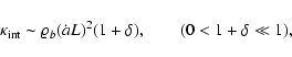
Eq. (8), is obeyed only at the largest densities, if at all. At
intermediate densities, Fig. 11 shows that the data
can be better fitted by the following polytropic-like behavior:
 |
(15) |
where the exponent
is detectably different from the virial
prediction ( ). A fit by eye yields the rough values
 ,
,
 ,
,
 - the amount of scatter does not allow a more precise
determination of ;
if the scatter is forgotten, it could even be
that
depends slightly on L, as seems to be the case when
n=-2, Fig. 10.
- the amount of scatter does not allow a more precise
determination of ;
if the scatter is forgotten, it could even be
that
depends slightly on L, as seems to be the case when
n=-2, Fig. 10.
At the intermediate time,
,
a similar behavior can be
detected, although the polytropic-like dependence (15)
can be discerned only with some difficulty,
Fig. 12. Apparently, the dynamical evolution has
not proceeded so far that the intermediate regime with
 can be clearly detected without interference of finite-mass effects:
they show up in this case as an artificial reduction of
when
is small enough, i.e., when there are only a few simulation
particles in the coarsening cells, see Fig. 12.
can be clearly detected without interference of finite-mass effects:
they show up in this case as an artificial reduction of
when
is small enough, i.e., when there are only a few simulation
particles in the coarsening cells, see Fig. 12.
![\begin{figure}
\par\resizebox{8.34cm}{!}{\includegraphics[clip]{figures/0566f10a...
...esizebox{8.34cm}{!}{\includegraphics[clip]{figures/0566f10c.eps}}
\end{figure}](/articles/aa/full/2004/20/aa0566/Timg166.gif) |
Figure 10:
Abscissa:
.
Ordinate:
![$\log [{\kappa}_{\rm int}/ \varrho_b
(\dot{a} L)^2]$](/articles/aa/full/2004/20/aa0566/img165.gif) .
Solid line: theoretical functional dependence,
Eq. (8). Plotted only coarsening lengths at the
latest time,
,
such that .
Solid line: theoretical functional dependence,
Eq. (8). Plotted only coarsening lengths at the
latest time,
,
such that
 .
For
clarity, the scatter bars are omitted; see
Fig. 11. .
For
clarity, the scatter bars are omitted; see
Fig. 11. |
| Open with DEXTER |
![\begin{figure}
\par\resizebox{8.34cm}{!}{\includegraphics[clip]{figures/0566f11a...
...esizebox{8.34cm}{!}{\includegraphics[clip]{figures/0566f11c.eps}}
\end{figure}](/articles/aa/full/2004/20/aa0566/Timg168.gif) |
Figure 11:
Same as Fig. 10, but now the ordinate is
![$\log[
{\kappa}_{\rm int}/ \varrho_b [\dot{a} L \sigma(L)]^2]$](/articles/aa/full/2004/20/aa0566/img167.gif) .
The solid lines ( .
The solid lines (
 )
have
and
,
,
The case n=-2 shows also the same data furnished with scatter
bars and shifted by a factor 103 for clarity. The scatter bars
of the other two cases are of the same size. )
have
and
,
,
The case n=-2 shows also the same data furnished with scatter
bars and shifted by a factor 103 for clarity. The scatter bars
of the other two cases are of the same size. |
| Open with DEXTER |
![\begin{figure}
\par\resizebox{8.8cm}{!}{\includegraphics[clip]{figures/0566f12.eps}}
\end{figure}](/articles/aa/full/2004/20/aa0566/Timg169.gif) |
Figure 12:
For n=+1,
,
:
the uppermost data are
scaled like in Fig. 10, the lowermost data like
in Fig. 11. For the other values of n, the
behavior of the data is the same. |
| Open with DEXTER |
4.4 CDM models
Regarding the CDM models, we have investigated only the relationship
in the nonlinear regime at the present epoch, in order
to assess the possibility of a polytropic-like dependence as in the
self-similar models. Figure 13 shows the measured
as a function of the density for the flat CDM model simulated in a box
of sidelength 128 Mpc. Now there is no reason to expect an exact
scaling behavior like (3) and the plots cannot be made
to collapse on a single function. Nevertheless, a dependence
fits well the data for
large enough,
with a scale-dependent exponent,  ,
which decreases with
decreasing L and ranges between 0 and 0.5 for the
lengths L which we probed
(
,
which decreases with
decreasing L and ranges between 0 and 0.5 for the
lengths L which we probed
( Mpc, see Sect. 3).
Figure 14 shows the measurements of
of the flat
CDM model in two different simulation boxes (128 and 512 Mpc
sidelength, respectively). The worse mass-resolution in the largest
box implies that, for a given L in the highly non-linear regime, the minimum
measurable value of
is larger. It also means that the absolute
value of
is smaller. The interesting finding is that, if
is multiplied by a factor 103, the plots corresponding to
different simulation boxes but to the same coarsening length superpose
each other.
The conclusions extracted from the open CDM models are qualitatively
identical to those reached with the flat CDM model, and the numerical
values for the exponent
are very similar.
![\begin{figure}
\par\resizebox{8.8cm}{!}{\includegraphics[clip]{figures/0566f13.eps}}
\end{figure}](/articles/aa/full/2004/20/aa0566/Timg173.gif) |
Figure 13:
Abscissa:
.
Ordinate:
 (arbitrary
normalization) for the flat CDM model in a box of sidelength 128 Mpc. For clarity, only some coarsening lengths are plotted
(decreasing top down). The solid lines (
)
have
and
(arbitrary
normalization) for the flat CDM model in a box of sidelength 128 Mpc. For clarity, only some coarsening lengths are plotted
(decreasing top down). The solid lines (
)
have
and  . . |
| Open with DEXTER |
5 Discussion and conclusions
In the previous section we have measured the macroscopic and the internal
kinetic energies of cubic cells as a function of time, cell size and
cell mass for different cosmological models. The use of self-similar
models simplifies the task of comparing with theoretical results, when
available. In particular, the scaling relationship (3)
is useful to assess unphysical dependences on the unavoidable
additional length scales introduced by the simulation procedure,
namely the box sidelength, R, and the mean interparticle separation, .
It must be noticed that, even when the results obey the
scaling (3), this does not imply irrelevance of these
extra length scales: one can conclude at most that R and could enter in the result solely as the combination  ,
or
equivalently, as N, the total particle number. We have not explored
explicitly the influence of such a dependence on N. Nevertheless,
from our results we can obtain some hints about how well they
reproduce the limit
,
or
equivalently, as N, the total particle number. We have not explored
explicitly the influence of such a dependence on N. Nevertheless,
from our results we can obtain some hints about how well they
reproduce the limit
 .
.
We first considered the unconstrained averages,
.
We find that
for
n=-2 suffers from strong finite-size effects in a predictable
manner. The mean internal kinetic energy,
,
however, is strongly affected by resolution effects, the
more so the larger n is, and its measurement is therefore
unreliable. Next we considered the constrained averages,
,
.
In general, they are much less affected by resolution effects, which are
"localized'' to very small mass densities or to the earliest time,
being more conspicuous for n=+1.
The macroscopic kinetic energy,
,
of
the case n=-2 depends strongly on R, as predicted
theoretically. However, this does not break self-similarity of the
amplitude of density fluctuations, as shown by Jain & Bertschinger (1998,1996),
or of
,
as argued in Sect. 2 and exemplified by our
results for
.
Relevant for the dynamical evolution of these
physical quantities is not the bulk velocity field, but the relative velocity (that is, the velocity gradient), which does not
suffer this R-dependence.
![\begin{figure}
\par\resizebox{8.8cm}{!}{\includegraphics[clip]{figures/0566f14.eps}}
\end{figure}](/articles/aa/full/2004/20/aa0566/Timg176.gif) |
Figure 14:
Abscissa:
.
Ordinate:
(arbitrary
normalization) for the flat CDM model in boxes of sidelength 128 Mpc and 512 Mpc, respectively. In the later case,
was multiplied by a factor 103. For clarity, only some
coarsening lengths are plotted. The solid lines (
)
have
and . |
| Open with DEXTER |
In the cases n=0,+1, the theoretical predictions and the
scaling (3) are well followed except at the earliest
times and smallest cell sizes, when resolution effects are expected to
be most important. An interesting result is the linear dependence of
with ,
Eq. (13), with a
proportionality factor which according to Fig. 7
does not seem to depend sensitively on the spectral index n.
Seto & Sugiyama (2001) have studied
in the cases n=0,+1 in the quasilinear
regime (
 ), which we have not
addressed at all.
), which we have not
addressed at all.
The internal kinetic energy,
,
is more sensitive to the small scale dynamics than
is;
correspondingly, resolution effects are found to be more important
than for
.
However, only at the earliest time and smallest coarsening cell
sizes for n=0,+1 do they render the results unreliable. That's why
the theoretical prediction for
in the linear regime
could not be tested when n=0,+1; when n=-2 the reason is that the
linear regime was not really probed, which can be traced back to a
finite-size effect.
In the nonlinear regime, the function
exhibits an
interesting behavior. The virial prediction, Eq. (8),
was observed only for n=0,+1 asymptotically in the large-end of the curves. Otherwise, a polytropic-like
dependence (15) was found to fit better the data, with an exponent which does
not seem to depend on time or coarsening length, only on the spectral index n. The same polytropic-like dependence is found for CDM models, albeit with a
scale-dependent exponent, confirming the results of an earlier work (Domínguez 2003). The
values of the exponent
for the CDM models analyzed here
and by Domínguez (2003) are consistent with each other and with
those of the self-similar models, in spite of the differences in the number of particles
in the simulations (and, compared to Domínguez 2003, the simulation
algorithm itself). This suggests that the
polytropic-like relation is not an artifact of the simulations, which
in this respect seem to reproduce acceptably the limit
.
Another hint in this direction is the simple relation which
connects the results of the CDM models in boxes of different size,
Sect. 4.4: in the larger box, R=512 Mpc, a coarsening cell
of a given mass contains less particles that in the smaller box,
R=128 Mpc. Nevertheless, this mass-resolution effect does not alter
the functional dependence
at all, and can be accounted
for by a scale-independent constant offset.
In the work by Kepner et al. (1997),
is also measured in CDM simulations (in their notation,
 ). They find a polytropic-like dependence too, but with
a slightly smaller exponent,
). They find a polytropic-like dependence too, but with
a slightly smaller exponent,
 (Kepner et al. 1997, Eqs. (17)-(18)).
We believe this discrepancy to be a consequence of
their simulation having too few particles (N=323): as a
consequence, they measured the function
with coarsening
cells having at most 100 particles (in one case); in many cases, the
cells have less than a few tens of particles (Kepner et al. 1997, Fig. 3).
For comparison, the polytropic-like dependence in
Fig. 13 is detected in coarsening cells containing a
number of particles spanning ranges as wide as 30-7000 or
500-30 000 (see also Domínguez 2003).
The work by Kepner et al. (1997) was motivated by comparison with redshift
surveys. It relied on the cosmic virial theorem and particular
emphasis was put on the dependence with cosmological parameters
(
(Kepner et al. 1997, Eqs. (17)-(18)).
We believe this discrepancy to be a consequence of
their simulation having too few particles (N=323): as a
consequence, they measured the function
with coarsening
cells having at most 100 particles (in one case); in many cases, the
cells have less than a few tens of particles (Kepner et al. 1997, Fig. 3).
For comparison, the polytropic-like dependence in
Fig. 13 is detected in coarsening cells containing a
number of particles spanning ranges as wide as 30-7000 or
500-30 000 (see also Domínguez 2003).
The work by Kepner et al. (1997) was motivated by comparison with redshift
surveys. It relied on the cosmic virial theorem and particular
emphasis was put on the dependence with cosmological parameters
( ,
,
 ). Our results show that departures from
the virial prediction are not small at all, so that the method devised
by Kepner et al. (1997) must be adjusted.
More generally, our results warn against a straightforward use of the
cosmic virial theorem to estimate cosmological parameters from
observations without first assessing that the employed observational
data do indeed pertain virialized structures.
). Our results show that departures from
the virial prediction are not small at all, so that the method devised
by Kepner et al. (1997) must be adjusted.
More generally, our results warn against a straightforward use of the
cosmic virial theorem to estimate cosmological parameters from
observations without first assessing that the employed observational
data do indeed pertain virialized structures.
In the work by Nagamine et al. (2001), the cosmic Mach number (=
in our notation, and
 in
theirs) is measured in a
in
theirs) is measured in a  CDM hydrodynamical simulation, for
three different length scales and as a function of the density. As a
side-result, they also find a polytropic-like dependence for the
velocity dispersion of groups of DM halos and galaxies (with
CDM hydrodynamical simulation, for
three different length scales and as a function of the density. As a
side-result, they also find a polytropic-like dependence for the
velocity dispersion of groups of DM halos and galaxies (with
 )
- the authors do not elaborate much on this result.
One must keep in mind that, compared to our simulations, theirs involves also the baryonic
component and the formation of galaxies, which can affect the velocity
dispersion (Tissera & Domínguez-Tenreiro 1998).
)
- the authors do not elaborate much on this result.
One must keep in mind that, compared to our simulations, theirs involves also the baryonic
component and the formation of galaxies, which can affect the velocity
dispersion (Tissera & Domínguez-Tenreiro 1998).
One can conceive two natural extreme cases of a polytropic-like
dependence: the "virial'' case,
,
when velocity
dispersion is fixed by the local mass density, and the "isothermal''
case,
 ,
when velocity dispersion is fixed by
an external cause, e.g. tidal forces, free flow,... The values of
that we
measure invariably fall between 0 and 1; the corresponding
relations
can be arguably understood as the outcome of
the competition of the two effects ("local virialization vs. global
thermalization''), whose relative strength varies with the spectral
index n and the cell size and mass. However, an elaborated theory is
required to lend support to this explanation,
the ultimate goal being the "postdiction'' of the
relation (15).
The value
,
when velocity dispersion is fixed by
an external cause, e.g. tidal forces, free flow,... The values of
that we
measure invariably fall between 0 and 1; the corresponding
relations
can be arguably understood as the outcome of
the competition of the two effects ("local virialization vs. global
thermalization''), whose relative strength varies with the spectral
index n and the cell size and mass. However, an elaborated theory is
required to lend support to this explanation,
the ultimate goal being the "postdiction'' of the
relation (15).
The value  was derived theoretically by Buchert & Domínguez (1998), but
we think this is irrelevant to our results, since
certain restrictive assumptions were made (vanishingly small and isotropic
velocity dispersion, approximately shear-free velocity field ),
which are unlikely to hold in the regime where we find the
polytropic-like dependence.
The results from the simulations cannot be explained by any theory
whose starting point is the usual thermodynamical theory or, more
generally, the (grand-)canonical ensemble of statistical mechanics
(Saslaw & Fang 1996; Hochberg & Pérez-Mercader 1996; de Vega et al. 1998), since in that framework the
kinetic energy is an extensive variable:
was derived theoretically by Buchert & Domínguez (1998), but
we think this is irrelevant to our results, since
certain restrictive assumptions were made (vanishingly small and isotropic
velocity dispersion, approximately shear-free velocity field ),
which are unlikely to hold in the regime where we find the
polytropic-like dependence.
The results from the simulations cannot be explained by any theory
whose starting point is the usual thermodynamical theory or, more
generally, the (grand-)canonical ensemble of statistical mechanics
(Saslaw & Fang 1996; Hochberg & Pérez-Mercader 1996; de Vega et al. 1998), since in that framework the
kinetic energy is an extensive variable:
 (T is the
kinetic temperature) and
(T is the
kinetic temperature) and  .
As a side-remark, we notice that Saslaw et al. (1990) compute the velocity
distribution allegedly in the framework of thermodynamics: but they
use contradictory arguments
and obtain instead that the kinetic energy scales like
.
As a side-remark, we notice that Saslaw et al. (1990) compute the velocity
distribution allegedly in the framework of thermodynamics: but they
use contradictory arguments
and obtain instead that the kinetic energy scales like  (that is, ), and a velocity distribution different
from the Maxwellian one characteristic of thermal equilibrium and
which should follow from the (grand-)canonical ensemble probability.
(that is, ), and a velocity distribution different
from the Maxwellian one characteristic of thermal equilibrium and
which should follow from the (grand-)canonical ensemble probability.
The discovered relationship
is useful for an improved
model of structure formation by gravitational instability
(Buchert & Domínguez 1998): the dust model (pressureless fluid) is added a term
proportional to the gradient of
(a kinetic pressure), in order
to account for the reaction of the dynamically generated velocity
dispersion on the evolution.
The evolution equation for the velocity field
 then
reads
then
reads
 |
(16) |
where the peculiar gravitational acceleration  is given by
Poisson's equation.
Further theoretical studies of this model
(Maartens et al. 1999; Buchert et al. 1999; Adler & Buchert 1999; Tatekawa et al. 2002; Morita & Tatekawa 2001) work with a
which
depends only on density, e.g. a pure polytropic-like dependence with
values of the exponent
in concordance with our measurements.
Our results show that the functional dependence of
on is somewhat more complicated than purely polytropic and changes with
time and coarsening length.
Nevertheless, since the term
is given by
Poisson's equation.
Further theoretical studies of this model
(Maartens et al. 1999; Buchert et al. 1999; Adler & Buchert 1999; Tatekawa et al. 2002; Morita & Tatekawa 2001) work with a
which
depends only on density, e.g. a pure polytropic-like dependence with
values of the exponent
in concordance with our measurements.
Our results show that the functional dependence of
on is somewhat more complicated than purely polytropic and changes with
time and coarsening length.
Nevertheless, since the term
 is a pressure, it opposes
compression in collapsing regions.
More can be learned about the behavior of this term when some
simplifications are introduced (Buchert et al. 1999; Buchert & Domínguez 1998): one assumes that
the evolution follows the dust model prediction in the form of the
Zel'dovich approximation (basically that
is a pressure, it opposes
compression in collapsing regions.
More can be learned about the behavior of this term when some
simplifications are introduced (Buchert et al. 1999; Buchert & Domínguez 1998): one assumes that
the evolution follows the dust model prediction in the form of the
Zel'dovich approximation (basically that
 )
"almost everywhere'', i.e., except near potential density
singularities where the effect of
becomes relevant.
One
can then apply boundary-layer theory to show (Domínguez 2000) that this
term does behave "adhesively'' and indeed succeeds in preventing the
formation of a singularity, provided
is a function of and
)
"almost everywhere'', i.e., except near potential density
singularities where the effect of
becomes relevant.
One
can then apply boundary-layer theory to show (Domínguez 2000) that this
term does behave "adhesively'' and indeed succeeds in preventing the
formation of a singularity, provided
is a function of and
 is a growing function of
(meaning
is a growing function of
(meaning  for a polytropic-like dependence). This behavior is robust
against the observed time-dependence in the relation
,
being much slower than the time-scale of collapse. One can conclude
that the dependence
for a polytropic-like dependence). This behavior is robust
against the observed time-dependence in the relation
,
being much slower than the time-scale of collapse. One can conclude
that the dependence
 measured in N-body simulations
leads to the same qualitative "adhesive'' behavior as the simpler
dependences addressed theoretically in the literature.
measured in N-body simulations
leads to the same qualitative "adhesive'' behavior as the simpler
dependences addressed theoretically in the literature.
When it comes to inserting our results in the theoretical
model (16),
there are some issues which we have not addressed but may be relevant
to a better understanding of the model.
First, it must be noticed that the
average relationship
does not mean in principle a
one-to-one dependence between
and ;
on the
contrary, the data scatter around the average dependence,
Fig. 11.
In fact, the derivation of Eq. (16) yields in reality a
term
 (Buchert & Domínguez 1998):
the influence of the scatter on the model outputs should be quantified
and, if proven relevant, incorporated in the model, e.g. as a noisy
source (Buchert et al. 1999).
Another issue of possible concern
is the amount of velocity dispersion
in the coarsening cells associated to "bound structures'' (as opposed
to the amount associated to particle flow between neighboring cells);
in this context, it would also be interesting to assess the
contribution to velocity dispersion from "ordered motion'', e.g. due
to a net angular momentum.
(Buchert & Domínguez 1998):
the influence of the scatter on the model outputs should be quantified
and, if proven relevant, incorporated in the model, e.g. as a noisy
source (Buchert et al. 1999).
Another issue of possible concern
is the amount of velocity dispersion
in the coarsening cells associated to "bound structures'' (as opposed
to the amount associated to particle flow between neighboring cells);
in this context, it would also be interesting to assess the
contribution to velocity dispersion from "ordered motion'', e.g. due
to a net angular momentum.
In conclusion, we have studied the density dependence of the
macroscopic and internal kinetic energies in coarsening cells. We
could identify the influence of finite-size and resolution effects on
the measured physical quantities. When these effects were irrelevant,
we could confirm some of the theoretical asymptotic predictions.
Finally, we found that in an intermediate range of densities, the
velocity dispersion scales as a power of the mass density, with an
exponent different from the virial prediction.
Acknowledgements
A.D. acknowledges support of the "Sonderforschungsbereich SFB 375 für Astro-Teilchenphysik der Deutschen
Forschungsgemeinschaft''. A.L.M. acknowledges support of US NSF
through grant AST0070702 and the National Center for Supercomputing
Applications (Urbana, Illinois, USA).
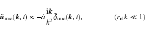
Appendix A: Estimates with the linear solution
In this Appendix we collect the mathematical calculations which lead
to Eqs. (4)-(6). The main idea is that
and
are determined by the dominant
contribution of modes in the linear regime when
,
so that
they can be estimated by inserting the linear solution in the
definitions (1). These definitions can be rewritten as
follows:
in terms of the formal microscopic fields
We introduce the Fourier transform of any spatial field
 ,
denoted by a tilde and defined as
,
denoted by a tilde and defined as
The velocity then reads
and the internal kinetic energy
 |
(A.1) |
Even if
,
these expressions contain contributions
from nonlinear modes (
 ). The hypothesis
(Sect. 2) is that these contributions are nevertheless
negligible compared to those from the linear modes (
). This implies
). The hypothesis
(Sect. 2) is that these contributions are nevertheless
negligible compared to those from the linear modes (
). This implies
 in the linear regime, and the growing linear solution in an Einstein-de Sitter background yields in turn
with
 .
Inserting these
linear relations in the definition (A.1) we obtain,
to lowest order in the inhomogeneities,
.
Inserting these
linear relations in the definition (A.1) we obtain,
to lowest order in the inhomogeneities,
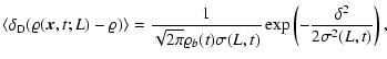
For Gaussian initial conditions, the average of
Eq. (2) can be easily computed using standard
techniques for the Gaussian functional integrals (e.g. Zinn-Justin 1996):
With these expressions, one recovers the result (6)
with the coefficients given by
![\begin{displaymath}
\langle K_{\rm int} \rangle (L, t) = \frac{1}{2} \varrho_b ...
...P(k)}{k^2} \left[1 - \vert\tilde{W}(L {\vec k})\vert^2\right],
\end{displaymath}](/articles/aa/full/2004/20/aa0566/img220.gif) |
(A.2) |
 |
(A.3) |
These integrals are IR-convergent provided
 , -3<n, since
 (
(
 the window function is normalized to unity
and decays fast enough at large distances). On the other hand, there
is an implicit ultraviolet (UV) cutoff,
the window function is normalized to unity
and decays fast enough at large distances). On the other hand, there
is an implicit ultraviolet (UV) cutoff,
 ,
because these
expressions have been derived for the linear regime.
The limit "
,
because these
expressions have been derived for the linear regime.
The limit "
 '' of the coefficient B is finite,
since we assume that
'' of the coefficient B is finite,
since we assume that
 fast enough
(
the window is smooth enough: the decay is
exponential for a Gaussian window, algebraic (
fast enough
(
the window is smooth enough: the decay is
exponential for a Gaussian window, algebraic (
 )
for a spherical top-hat window).
is however
UV-convergent only if
)
for a spherical top-hat window).
is however
UV-convergent only if
 , n<-1,
indicating that it is determined by nonlinear modes when n>-1.
, n<-1,
indicating that it is determined by nonlinear modes when n>-1.
A similar reasoning can be repeated for the macroscopic kinetic
energy: inserting the linear relationships in the definition
 one gets
which is IR-divergent in the range of spectral indices -3<n<-1.
- Adler, S., &
Buchert, T. 1999, A&A, 343, 317 [NASA ADS]
- Bernardeau, F.,
Colombi, S., Gaztañaga, E., & Scoccimarro, R. 2002,
Phys. Rep., 367, 1 [NASA ADS] [MathSciNet] (In the text)
- Buchert, T., &
Domínguez, A. 1998, A&A, 335, 395 [NASA ADS]
- Buchert, T.,
Domínguez, A., & Pérez-Mercader, J. 1999, A&A,
349, 343 [NASA ADS]
- de Vega, H.,
Sánchez, N., & Combes, F. 1998, ApJ, 500, 8 [NASA ADS] [CrossRef]
- Dekel, A. 1994,
ARA&A, 32, 371 [NASA ADS] (In the text)
- Domínguez, A.
1999, Ph.D. Thesis, Univ. Autónoma de Madrid
- Domínguez, A.
2000, Phys. Rev. D, 62, 103501 [NASA ADS] [CrossRef]
- Domínguez, A.
2002, MNRAS, 334, 435 [NASA ADS] [CrossRef]
- Domínguez, A.
2003, Astron. Nachr., 324, 560 [NASA ADS] [CrossRef]
- Feldman, H.,
Juszkiewicz, R., Ferreira, P., et al. 2003, ApJ, 596,
L131 [NASA ADS] [CrossRef]
- Gurbatov, S. N.,
Saichev, A. I., & Shandarin, S. F. 1989, MNRAS, 236,
385 [NASA ADS]
- Hochberg, D., &
Pérez-Mercader, J. 1996, Gen. Rel. Grav., 28, 1427 [NASA ADS]
- Jain, B., &
Bertschinger, E. 1996, ApJ, 456, 43 [NASA ADS] [CrossRef]
- Jain, B., &
Bertschinger, E. 1998, ApJ, 509, 517 [NASA ADS] [CrossRef]
- Kepner, J. V.,
Summers, F. J., & Strauss, M. A. 1997, New Astron.,
2, 165 [NASA ADS] [CrossRef]
- Klypin, A., &
Holtzmann, J. 1997 [arXiv:astro-ph/9712217]
(In the text)
- Knebe, A., &
Müller, V. 1999, A&A, 341, 1 [NASA ADS] (In the text)
- Kofman, L., Pogosyan,
D., Shandarin, S. F., & Melott, A. L. 1992, ApJ, 393,
437 [NASA ADS] [CrossRef]
- Kofman, L., &
Shandarin, S. 1988, Nature, 334, 129 [NASA ADS] [CrossRef]
- Maartens, R., Triginer,
J., & Matravers, D. R. 1999, Phys. Rev. D, 60,
103503 [NASA ADS] [CrossRef]
- Melott, A. L.,
& Shandarin, S. F. 1993, ApJ, 410, 469 [NASA ADS] [CrossRef] (In the text)
- Melott, A. L.,
Shandarin, S. F., & Weinberg, D. H. 1994, ApJ, 428,
28 [NASA ADS] [CrossRef]
- Morita, M., &
Tatekawa, T. 2001, MNRAS, 328, 815 [NASA ADS] [CrossRef]
- Nagamine, K., Ostriker,
J. P., & Cen, R. 2001, ApJ, 553, 513 [NASA ADS] [CrossRef]
- Ostriker, J. P.,
& Suto, Y. 1990, ApJ, 348, 378 [NASA ADS] [CrossRef] (In the text)
- Padmanabhan, T. 1995,
Structure Formation in the Universe (Cambridge Univ. Press)
- Peebles, P. J. E.
1980, The Large-Scale Structure of the Universe (Princeton Univ.
Press)
(In the text)
- Sahni, V., & Coles,
P. 1995, Phys. Rep., 262, 1 [NASA ADS]
- Saslaw, W. C.,
Chitre, S. M., Itoh, M., & Inagaki, S. 1990, ApJ, 365,
419 [NASA ADS] [CrossRef] (In the text)
- Saslaw, W. C.,
& Fang, F. 1996, ApJ, 460, 16 [NASA ADS] [CrossRef]
- Sathyaprakash,
B. S., Sahni, V., Munshi, D., Pogosyan, D., & Melott,
A. L. 1995, MNRAS, 275, 463 [NASA ADS]
- Seto, N., &
Sugiyama, N. 2001, ApJ, 558, 505 [NASA ADS] [CrossRef] (In the text)
- Strauss, M. A.,
Ostriker, J. P., & Cen, R. 1998, ApJ, 494, 20 [NASA ADS] [CrossRef]
- Tatekawa, T., Suda, M.,
Maeda, K., Morita, M., & Anzai, H. 2002,
Phys. Rev. D, 66, 064014 [NASA ADS] [CrossRef]
- Tissera, P. B.,
& Domínguez-Tenreiro, R. 1998, MNRAS, 297, 177 [NASA ADS] [CrossRef] (In the text)
- Watkins, R., Feldman,
H. A., Chambers, S. W., Gorman, P., & Melott,
A. L. 2002, ApJ, 564, 534 [NASA ADS] [CrossRef] (In the text)
- Zinn-Justin, J. 1996,
Quantum field theory and critical phenomena (Oxford: Clarendon
Press)
(In the text)
Copyright ESO 2004
![\begin{displaymath}\varrho ({\vec x}, t; L) = \frac{m}{[a(t) L]^3} \sum_{\alpha=...
...} ~
W \left({{\vec x}-{\vec x}_\alpha (t) \over L} \right),
\end{displaymath}](/articles/aa/full/2004/20/aa0566/img46.gif)
![\begin{displaymath}K_{\rm int} ({\vec x}, t; L) = \frac{m}{2 [a(t) L]^3} \sum_{\...
...2
W \left({{\vec x}-{\vec x}_\alpha (t) \over L} \right)\cdot
\end{displaymath}](/articles/aa/full/2004/20/aa0566/img48.gif)
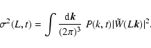
![\begin{figure}
\par\resizebox{8.8cm}{!}{\includegraphics[clip]{figures/0566f1.eps}}
\end{figure}](/articles/aa/full/2004/20/aa0566/img86.gif)
![\begin{figure}
\par\resizebox{8.8cm}{!}{\includegraphics[clip]{figures/0566f2a.e...
...r\resizebox{8.8cm}{!}{\includegraphics[clip]{figures/0566f2c.eps}}
\end{figure}](/articles/aa/full/2004/20/aa0566/img140.gif)
![\begin{figure}
\par\resizebox{8.6cm}{!}{\includegraphics[clip]{figures/0566f3a.e...
... \resizebox{8.6cm}{!}{\includegraphics[clip]{figures/0566f3c.eps}}
\end{figure}](/articles/aa/full/2004/20/aa0566/img143.gif)
![\begin{figure}
\par\resizebox{8.6cm}{!}{\includegraphics[clip]{figures/0566f4a.e...
...\resizebox{8.6cm}{!}{\includegraphics[clip]{figures/0566f4b.eps}}
\end{figure}](/articles/aa/full/2004/20/aa0566/img146.gif)
![\begin{figure}
\par\resizebox{8.4cm}{!}{\includegraphics[clip]{figures/0566f5.eps}}
\end{figure}](/articles/aa/full/2004/20/aa0566/img151.gif)
![\begin{figure}
\par\resizebox{8.5cm}{!}{\includegraphics[clip]{figures/0566f6a.e...
...\resizebox{8.5cm}{!}{\includegraphics[clip]{figures/0566f6b.eps}}
\end{figure}](/articles/aa/full/2004/20/aa0566/img157.gif)
![\begin{figure}
\par\resizebox{8.4cm}{!}{\includegraphics[clip]{figures/0566f7.eps}}
\end{figure}](/articles/aa/full/2004/20/aa0566/img158.gif)
![\begin{figure}
\par\resizebox{8.6cm}{!}{\includegraphics[clip]{figures/0566f8.eps}}
\end{figure}](/articles/aa/full/2004/20/aa0566/img160.gif)
![\begin{figure}
\par\resizebox{8.6cm}{!}{\includegraphics[clip]{figures/0566f9a.e...
...\resizebox{8.6cm}{!}{\includegraphics[clip]{figures/0566f9b.eps}}
\end{figure}](/articles/aa/full/2004/20/aa0566/img162.gif)
![\begin{figure}
\par\resizebox{8.34cm}{!}{\includegraphics[clip]{figures/0566f10a...
...esizebox{8.34cm}{!}{\includegraphics[clip]{figures/0566f10c.eps}}
\end{figure}](/articles/aa/full/2004/20/aa0566/img166.gif)
![\begin{figure}
\par\resizebox{8.34cm}{!}{\includegraphics[clip]{figures/0566f11a...
...esizebox{8.34cm}{!}{\includegraphics[clip]{figures/0566f11c.eps}}
\end{figure}](/articles/aa/full/2004/20/aa0566/img168.gif)
![\begin{figure}
\par\resizebox{8.8cm}{!}{\includegraphics[clip]{figures/0566f12.eps}}
\end{figure}](/articles/aa/full/2004/20/aa0566/img169.gif)
![\begin{figure}
\par\resizebox{8.8cm}{!}{\includegraphics[clip]{figures/0566f13.eps}}
\end{figure}](/articles/aa/full/2004/20/aa0566/img173.gif)
![\begin{figure}
\par\resizebox{8.8cm}{!}{\includegraphics[clip]{figures/0566f14.eps}}
\end{figure}](/articles/aa/full/2004/20/aa0566/img176.gif)
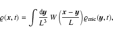
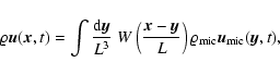
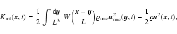
![\begin{displaymath}\times\left[ \tilde{\vec u}_{\rm mic} ({\vec q}, t) \cdot \ti...
...ot \tilde{\vec u}({\vec p}, t) \tilde{W} (L {\vec k})\right].
\end{displaymath}](/articles/aa/full/2004/20/aa0566/img210.gif)