A&A 418, 53-65 (2004)
DOI: 10.1051/0004-6361:20034541
Monte Carlo simulations of the halo white dwarf population
E. García-Berro1,2 -
S. Torres1 -
J. Isern2,3 -
A. Burkert4
1 - Departament de Física Aplicada, Escola Politécnica
Superior de Castelldefels, Universitat Politècnica de
Catalunya, Avda. del Canal Olímpic s/n, 08860
Castelldefels, Spain
2 -
Institute for Space Studies of Catalonia, c/Gran Capità
2-4, Edif. Nexus 104, 08034 Barcelona, Spain
3 -
Institut de Ciències de l'Espai, CSI
4 -
Max-Planck-Institut für Astronomie, Koenigstuhl 17,
69117 Heidelberg, Germany
Received 20 October 2003 / Accepted 24 December 2003
Abstract
The interpretation of microlensing results towards the Large
Magellanic Cloud (LMC) still remains controversial. While white
dwarfs have been proposed to explain these results and, hence, to
contribute significantly to the mass budget of our Galaxy, there are
also several constraints on the role played by white dwarfs. In this
paper we analyze self-consistently and simultaneously four different
results, namely, the local halo white dwarf luminosity function, the
microlensing results reported by the MACHO team towards the LMC, the
results of Hubble Deep Field (HDF) and the results of the EROS
experiment, for several initial mass functions and halo ages. We find
that the proposed log-normal initial mass functions do not contribute
to solve the problem posed by the observed microlensing events and,
moreover, they overproduce white dwarfs when compared to the results
of the HDF and of the EROS survey. We also find that the contribution
of hydrogen-rich white dwarfs to the dynamical mass of the halo of the
Galaxy cannot be more than  4%.
4%.
Key words: stars: white dwarfs - stars: luminosity function, mass
function - Galaxy: stellar content - Galaxy: dark matter -
Galaxy: structure - Galaxy: halo
White dwarfs are the most common remnants of stellar evolution. Since
white dwarfs are long-lived objects and the physical processes
governing their evolution are relatively well understood - at least
up to moderately low luminosities - they provide us with an
invaluable tool to study the evolution and structure of our Galaxy.
In fact, the disk white dwarf luminosity function has become an
important tool to determine some properties of the local neighborhood,
such as its age (Winget et al. 1987; García-Berro et al.
1988;
Hernanz et al. 1994), or the past history of the star formation rate
(Noh & Scalo 1990; Díaz-Pinto et al. 1994; Isern et al.
1995a,b). This has been possible because now we have improved
observational luminosity functions (Liebert et al. 1988;
Oswalt et al. 1996; Leggett et al. 1998) and because we
have reliable cooling sequences - see, for instance, Salaris et al.
(2000), and references therein.
Although the situation for the disk white dwarf population seems to be
clear and well understood, this is not the case for the halo white
dwarf population. The discovery of microlenses towards the Large
Magellanic Cloud (Alcock et al. 1996, 2000;
Lasserre et al. 2001) has generated a large controversy about the possibility
that white dwarfs could be responsible for these microlensing events
and, thus, could provide a significant contribution to the mass budget
of our Galactic halo. Nevertheless, white dwarfs as dark matter
candidates are not free of problems, since an excess of this kind of
object would necessarily imply an overproduction of low-mass main
sequence red dwarfs and high-mass stars that could eventually explode
as type II supernovae. To solve these problems Adams & Laughlin
(1996) and Chabrier et al. (1996) proposed
non-standard initial mass functions in which the formation of both
low and high mass stars was suppressed. Besides the lack of evidence
favoring such ad-hoc initial mass functions, they are not free of
problems either. In particular, the formation of a typical (
 )
white dwarf is accompanied by the injection into
the interstellar medium of a sizeable amount of mass (
)
white dwarf is accompanied by the injection into
the interstellar medium of a sizeable amount of mass (
 on average). Since type II supernovae are suppressed in
ad-hoc initial mass functions, there is not enough energy to eject
this matter into the intergalactic medium and the ejected mass, which
is significantly contaminated by metals (Abia et al. 2001; Gibson &
Mould 1997), cannot be accomodated in the Galaxy (Isern et al. 1998).
Finally, an excess of white dwarfs also translates into an excess of
binaries containing such stars with the subsequent increase of type Ia
supernova rates which, ultimately, results in an increase in the
abundances of the elements of the iron peak (Canal et al. 1997). All these arguments have forced the search for
other possible explanations, such as self-lensing in the LMC (Wu
1994; Salati et al. 1999), or background objects (Green & Jedamzik
2002) which have not been totally discarded yet.
on average). Since type II supernovae are suppressed in
ad-hoc initial mass functions, there is not enough energy to eject
this matter into the intergalactic medium and the ejected mass, which
is significantly contaminated by metals (Abia et al. 2001; Gibson &
Mould 1997), cannot be accomodated in the Galaxy (Isern et al. 1998).
Finally, an excess of white dwarfs also translates into an excess of
binaries containing such stars with the subsequent increase of type Ia
supernova rates which, ultimately, results in an increase in the
abundances of the elements of the iron peak (Canal et al. 1997). All these arguments have forced the search for
other possible explanations, such as self-lensing in the LMC (Wu
1994; Salati et al. 1999), or background objects (Green & Jedamzik
2002) which have not been totally discarded yet.
The suggestion of the MACHO team (Alcock et al. 1997, 2000) that
white dwarfs contribute significantly to the mass budget of the
Galactic halo has motivated a large number of observational searches
(Knox et al. 1999; Ibata et al. 1999; Oppenheimer et al.
2001; Majewski & Siegel 2002; Nelson et al. 2002) for these elusive
white dwarfs. Also several theoretical works (Reylé et al. 2001; Flynn et al. 2003) have analyzed this
possibility. However, the controversy of whether or not white dwarfs
can provide a significant contribution to the Galactic dark matter is
still open and deserves some more attention. In Isern et al. (1998)
we analyzed the halo white dwarf population. In particular, we
computed, assuming a standard initial mass function and updated models
of white dwarf cooling, the expected luminosity function, both in
luminosity and in visual magnitude, for different star formation
rates. We showed that a deep enough survey (limiting magnitude
 20) could provide important information about the halo age and the
duration of the formation stage. We also showed that the number of
white dwarfs produced using the proposed biased IMFs could not
represent a large fraction of the halo dark matter if they were
constrained by the observed luminosity function of halo white dwarfs.
However, within the approach adopted there the biases introduced by
the sample selection procedures were not taken into account. More
recently, we have analyzed (Torres et al. 2002) the sample of
Oppenheimer et al. (2001). In this paper we examine in detail the
results of the MACHO team (Alcock et al. 2000) carefully taking into
account the observational biases, thus updating our previous papers on
this subject. We also study the number of white dwarfs that could be
potentially found in the HDF (Ibata et al. 1999). Finally we also
analyze the very recent observational results of the EROS team
(Goldman et al. 2002), which set a very stringent upper limit to the
white dwarf content of the Galactic halo. All these analyses are done
by making use of a Monte Carlo simulator (García-Berro et al.
1999; Torres et al. 1998). This is an important issue since white
dwarf populations are usually drawn from kinematically selected
samples (white dwarfs with relatively high proper motions).
Therefore, some kinematical biases or distortions are expected. A
Monte Carlo simulation of a model population of white dwarfs is
expected to allow the biases and effects of sample selection to be
taken into account, so the properties of the real sample could be
corrected - or, at least, correctly interpreted - provided that a
detailed simulation from the very early stages of source selection is
performed accurately. Our paper is organized as follows. In section
Sect. 2 we describe in full detail the Monte Carlo code. In Sect. 3 we
present the results, whereas in Sect. 4 our conclusions are summarized.
20) could provide important information about the halo age and the
duration of the formation stage. We also showed that the number of
white dwarfs produced using the proposed biased IMFs could not
represent a large fraction of the halo dark matter if they were
constrained by the observed luminosity function of halo white dwarfs.
However, within the approach adopted there the biases introduced by
the sample selection procedures were not taken into account. More
recently, we have analyzed (Torres et al. 2002) the sample of
Oppenheimer et al. (2001). In this paper we examine in detail the
results of the MACHO team (Alcock et al. 2000) carefully taking into
account the observational biases, thus updating our previous papers on
this subject. We also study the number of white dwarfs that could be
potentially found in the HDF (Ibata et al. 1999). Finally we also
analyze the very recent observational results of the EROS team
(Goldman et al. 2002), which set a very stringent upper limit to the
white dwarf content of the Galactic halo. All these analyses are done
by making use of a Monte Carlo simulator (García-Berro et al.
1999; Torres et al. 1998). This is an important issue since white
dwarf populations are usually drawn from kinematically selected
samples (white dwarfs with relatively high proper motions).
Therefore, some kinematical biases or distortions are expected. A
Monte Carlo simulation of a model population of white dwarfs is
expected to allow the biases and effects of sample selection to be
taken into account, so the properties of the real sample could be
corrected - or, at least, correctly interpreted - provided that a
detailed simulation from the very early stages of source selection is
performed accurately. Our paper is organized as follows. In section
Sect. 2 we describe in full detail the Monte Carlo code. In Sect. 3 we
present the results, whereas in Sect. 4 our conclusions are summarized.
Table 1:
The different IMFs used in this paper.
In this section we discuss the main ingredients of our Monte Carlo
simulator. Since we want to self-consistently simulate simultaneously
four different results, namely, the local halo white dwarf luminosity
function, the microlensing results towards the LMC, the results of the
HDF, and the results of the EROS team, and each one of these
simulations requires slightly different inputs, we will describe them
in separate subsections. All of them, however, share some common
ingredients like a random number generator, which is always at the
heart of any Monte Carlo simulation. We have used a random number
generator algorithm (James 1990) which provides a uniform probability
density within the interval (0,1) and ensures a repetition period of
1018, which is enough for our purposes. Each one of the
Monte Carlo simulations discussed in Sect. 3 below consists of an
ensemble of 40 independent realizations of the synthetic white dwarf
population, for which the average of any observational quantity along
with its corresponding standard deviation were computed. Here the
standard deviation means the ensemble mean of the sample dispersions
for a typical sample.
We have considered a typical spherically symmetric halo. One of the
most commonly used models of this type is the isothermal sphere. The
density profile of the luminous halo is given by the law
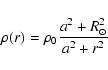 |
(1) |
where
 kpc is the core radius,
  is the
local halo density and
is the
local halo density and
 kpc is the galactocentric
distance of the Sun. We randomly choose three numbers for the
spherical coordinates
kpc is the galactocentric
distance of the Sun. We randomly choose three numbers for the
spherical coordinates
 of each star of the sample
within approximately 350 pc from the sun, according to Eq. (1).
Afterwards we draw another pseudo-random number in order to obtain the
main sequence mass of each star, according to one of the four model
initial mass functions that will be studied here. These initial mass
functions are, respectively, a standard IMF (Scalo 1998), the biased IMF of Adams & Laughlin (1996) and the two ad-hoc IMFs proposed by
Chabrier et al. (1996). All these mass functions are summarized in
Table 1. Once the mass of the progenitor of the white dwarf is known
we randomly choose the time at which each star was born (
of each star of the sample
within approximately 350 pc from the sun, according to Eq. (1).
Afterwards we draw another pseudo-random number in order to obtain the
main sequence mass of each star, according to one of the four model
initial mass functions that will be studied here. These initial mass
functions are, respectively, a standard IMF (Scalo 1998), the biased IMF of Adams & Laughlin (1996) and the two ad-hoc IMFs proposed by
Chabrier et al. (1996). All these mass functions are summarized in
Table 1. Once the mass of the progenitor of the white dwarf is known
we randomly choose the time at which each star was born ( ).
For this purpose we assume that the halo was formed 14 Gyr ago (see,
however, Sect. 3 below) in an intense burst of star formation of
duration 1 Gyr. Given the age of the halo,
and the
main sequence lifetime as a function of the mass in the main sequence
(Iben & Laughlin 1989) we know which stars have had time enough to
become white dwarfs, and given a set of cooling sequences (Salaris et al. 2000) and the initial to final mass relationship (Iben &
Laughlin 1989), which are their luminosities.
).
For this purpose we assume that the halo was formed 14 Gyr ago (see,
however, Sect. 3 below) in an intense burst of star formation of
duration 1 Gyr. Given the age of the halo,
and the
main sequence lifetime as a function of the mass in the main sequence
(Iben & Laughlin 1989) we know which stars have had time enough to
become white dwarfs, and given a set of cooling sequences (Salaris et al. 2000) and the initial to final mass relationship (Iben &
Laughlin 1989), which are their luminosities.
The velocity distribution has been modeled according to a Gaussian law
(Binney & Tremaine 1987):
![\begin{displaymath}f(v_r,v_t)=\frac{1}{(2\pi)^{3/2}}\frac{1}{\sigma_r\sigma_t^2}...
...c{v_r^2}{\sigma_t^2}+\frac{v_{t}^2}
{\sigma_t^2}\right)\right]
\end{displaymath}](/articles/aa/full/2004/16/aa0541/img14.gif) |
(2) |
where  and
and  - the radial and the
tangential velocity dispersion, respectively - are related by the
following expression:
- the radial and the
tangential velocity dispersion, respectively - are related by the
following expression:
 |
(3) |
which, to a first approximation, leads to
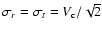 .
- see, for instance, Binney &
Tremaine (1987). For the calculations reported here we have adopted a
circular velocity
.
- see, for instance, Binney &
Tremaine (1987). For the calculations reported here we have adopted a
circular velocity
 km s-1. From these velocities we
obtain the heliocentric velocities by adding the velocity of the LSR
km s-1. From these velocities we
obtain the heliocentric velocities by adding the velocity of the LSR
 km s-1 and the peculiar velocity of the sun:
 km s-1 (Dehnen & Binney
1998). Since white dwarfs usually do not have determinations of the
radial component of the velocity, when needed for the observational
comparison the radial velocity is eliminated. Moreover, we only
consider stars with tangential velocities in the range
km s-1 (Dehnen & Binney
1998). Since white dwarfs usually do not have determinations of the
radial component of the velocity, when needed for the observational
comparison the radial velocity is eliminated. Moreover, we only
consider stars with tangential velocities in the range
 km s-1. Stars with velocities smaller than 250 km s-1would not be considered as halo members, whereas stars with velocities
larger than 750 km s-1 would have velocities exceeding 1.5 times the
escape velocity, which we obtain from Binney & Tremaine (1987):
km s-1. Stars with velocities smaller than 250 km s-1would not be considered as halo members, whereas stars with velocities
larger than 750 km s-1 would have velocities exceeding 1.5 times the
escape velocity, which we obtain from Binney & Tremaine (1987):
![\begin{displaymath}v_{\rm e}^2=2V_{\rm c}^2[1+\ln(r_*/r)]
\end{displaymath}](/articles/aa/full/2004/16/aa0541/img23.gif) |
(4) |
where
 kpc is the radius of the galactic halo.
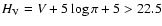
To build the white dwarf luminosity function using the
 method (Schmidt 1968) a smaller sample of white dwarfs must be culled
from the original sample and to do this a set of restrictions in
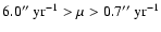
visual magnitude and proper motion must be adopted. The restriction
in magnitude will be discussed in Sect. 3 below. Regarding the proper
motion cut we have chosen
method (Schmidt 1968) a smaller sample of white dwarfs must be culled
from the original sample and to do this a set of restrictions in
visual magnitude and proper motion must be adopted. The restriction
in magnitude will be discussed in Sect. 3 below. Regarding the proper
motion cut we have chosen
 yr-1 as
in Oswalt et al. (1996) and in García-Berro et al. (1999).
Besides, the
method requires that all the objects
belonging to the restricted sample must have known parallaxes. This,
in turn, means that all the white dwarfs belonging to this sample are
within a sphere of radius of roughly 200 pc centered on the location
of the sun.
yr-1 as
in Oswalt et al. (1996) and in García-Berro et al. (1999).
Besides, the
method requires that all the objects
belonging to the restricted sample must have known parallaxes. This,
in turn, means that all the white dwarfs belonging to this sample are
within a sphere of radius of roughly 200 pc centered on the location
of the sun.
In order to produce a set of microlensing events towards the LMC we
also need to simulate the characteristics of the white dwarf
population towards the LMC. For this purpose we generate the three
galactic coordinates (r,l,b) of the white dwarfs of the galactic
halo inside a small pencil of
 centered in
the LMC location,
centered in
the LMC location,
 .
The l and bdistributions are practically uniform in this small window. The
radial coordinate is always smaller than the outer limit of the halo
(r<41 kpc) and according to the radial distribution
.
The l and bdistributions are practically uniform in this small window. The
radial coordinate is always smaller than the outer limit of the halo
(r<41 kpc) and according to the radial distribution
 |
(5) |
where
 - see, however, Sect. 3.7. We have chosen
this distribution instead of that of Eq. (1) because in this way
the number of microlensing events is maximized. In fact the mass
distribution of microlenses does not necessarily follow the mass
distribution of the luminous halo. However, in a first step (see Sect. 3.6 below), we have normalized the density of white dwarfs obtained
from this distribution to the white dwarf density of the local
neighborhood,
- see, however, Sect. 3.7. We have chosen
this distribution instead of that of Eq. (1) because in this way
the number of microlensing events is maximized. In fact the mass
distribution of microlenses does not necessarily follow the mass
distribution of the luminous halo. However, in a first step (see Sect. 3.6 below), we have normalized the density of white dwarfs obtained
from this distribution to the white dwarf density of the local
neighborhood,
 pc-3 for
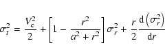
 (Torres et al. 1998). The velocity dispersions in
this case are determined from Markovic & Sommer-Larsen (1996).
For the radial velocity dispersion we have:
(Torres et al. 1998). The velocity dispersions in
this case are determined from Markovic & Sommer-Larsen (1996).
For the radial velocity dispersion we have:
![\begin{displaymath}\sigma_r^2=\sigma_0^2+\sigma_+^2\left[\frac{1}{2}
-\frac{1}{\pi}\arctan\left(\frac{r-r_0}{l}\right)\right]
\end{displaymath}](/articles/aa/full/2004/16/aa0541/img33.gif) |
(6) |
where
 ,
,
 ,
r0=10.5 kpc and l=5.5 kpc. The tangential
dispersion is given by:
,
r0=10.5 kpc and l=5.5 kpc. The tangential
dispersion is given by:
 |
(7) |
where
![\begin{displaymath}r\frac{{\rm d}\sigma_r^2}{{\rm d}r}=
-\frac{1}{\pi}\frac{r}{l}\frac{\sigma_+^2}{1+[(r-r_0)/l]^2}\cdot
\end{displaymath}](/articles/aa/full/2004/16/aa0541/img37.gif) |
(8) |
In order to decide which white dwarf could potentially produce a
microlensing event a magnitude cut must be adopted. If the white
dwarf is brighter than this limiting magnitude it could be potentially
detected and, consequently, would not be a genuine microlensing event.
We have explored a wide range of possibilities, namely
 and
and
 ,
but, as
a fiducial value, we have taken
,
but, as
a fiducial value, we have taken
 ,
which is the value adopted by Alcock et al. (2000). We also need to
simulate the population of stars of the LMC itself. In order to
produce such a population we distribute the number of monitored point
sources (
,
which is the value adopted by Alcock et al. (2000). We also need to
simulate the population of stars of the LMC itself. In order to
produce such a population we distribute the number of monitored point
sources (
 )
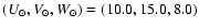
according to the LMC model of Gyuk et al. (2000). That is, we have adopted a scale lenght,
)
according to the LMC model of Gyuk et al. (2000). That is, we have adopted a scale lenght,
 ,
a scale height
,
a scale height
 ,
an inclination
angle
,
an inclination
angle
 ,
a distance
,
a distance
 ,
a position angle,
,
a position angle,
 ,
and a tangential heliocentric velocity,
,
and a tangential heliocentric velocity,
 .
The next step is to determine if there
exists a white dwarf in the line of sight to a given simulated star in
the LMC. We consider a white dwarf to be responsible of a
microlensing event if the angular distance between the white dwarf and
the monitored star is smaller than the Einstein radius
.
The next step is to determine if there
exists a white dwarf in the line of sight to a given simulated star in
the LMC. We consider a white dwarf to be responsible of a
microlensing event if the angular distance between the white dwarf and
the monitored star is smaller than the Einstein radius
 ,
where
,
where  is the Einstein radius and
 is the distance between the observer and the lens. This,
of course, can happen at any time during the total monitoring period
of 5.7 yr, due to the proper motion of the lenses, which is obtained
from the previous equations.
is the distance between the observer and the lens. This,
of course, can happen at any time during the total monitoring period
of 5.7 yr, due to the proper motion of the lenses, which is obtained
from the previous equations.
The optical depth is obtained, following Alcock et al. (2000), using
the expression
 |
(9) |
where
 is the total exposure (in
star-years),
is the total exposure (in
star-years),  is the Einstein ring diameter crossing time,
and
is the Einstein ring diameter crossing time,
and
 is the detection efficiency. The
detection efficiency has been modelled as:
is the detection efficiency. The
detection efficiency has been modelled as:
 |
(10) |
where
 days. This expression provides a good
fit to the results of Alcock et al. (2000).
days. This expression provides a good
fit to the results of Alcock et al. (2000).
For the simulation of the HDF we have distributed stars in a window of
 centered around
 .
The radial distribution is, again, according to Eq. (5) within the outer halo limit. The velocities are consequently
drawn from Eqs. (2) and (6) to (8). This simulation has been
also normalized to the local density given by the halo simulation.
.
The radial distribution is, again, according to Eq. (5) within the outer halo limit. The velocities are consequently
drawn from Eqs. (2) and (6) to (8). This simulation has been
also normalized to the local density given by the halo simulation.
Finally, for the simulation of the EROS results we have distributed
stars in a window of
 in the Southern Galactic
Hemisphere (
in the Southern Galactic
Hemisphere (
 ), in the following
strips along the
), in the following
strips along the  coordinate,
 wide:
wide:
 at
at
 ,
,
 at
at
 and
and
 at
at
 ,
and
,
and
 in the Northern Galactic Hemisphere (
 )
with
)
with
 at
at
 and
and
 at
at
 .
The radial distribution and the
velocity distribution are, again, the same used for the HDF
simulation. Also, the density of white dwarfs has been normalized to
the local density given by the halo simulation.
.
The radial distribution and the
velocity distribution are, again, the same used for the HDF
simulation. Also, the density of white dwarfs has been normalized to
the local density given by the halo simulation.
![\begin{figure}
\par\includegraphics[width=8.8cm,clip]{0541fig01.ps}
\end{figure}](/articles/aa/full/2004/16/aa0541/Timg75.gif) |
Figure 1:
Luminosity function of halo white dwarfs for several limiting
magnitudes. |
| Open with DEXTER |
One of the most serious problems that is found when determining the
observational white dwarf luminosity function of halo white dwarfs is
that the real limiting magnitude used in these studies is highly
uncertain. We have conducted a series of simulations with different
limiting magnitudes to determine which would be the limiting magnitude
able to reproduce the observational luminosity function. In Fig. 1
we show the white dwarf luminosity functions obtained for several
limiting magnitudes (16, 17, 18 and
 )
as solid lines.
The luminosity function of Torres et al. (1998) is shown as a dashed
line for comparison purposes. Each panel is clearly marked with its
corresponding limiting magnitude. The adopted halo age in all the
cases was 14 Gyr. Also the adopted IMF is the standard one in all
four simulations. The error bars of each luminosity bin were computed
according to Liebert et al. (1988): the contribution of each star to
the total error budget in its bin is conservatively estimated to be
the same amount that contributes to the resulting density; the partial
contributions of each star in the bin are squared and then added, the
final error being the square root of this value. This procedure is
followed for each of the 40 realizations of the Monte Carlo
simulation. After doing this the ensemble average of the dispersions
is computed. Obviously the larger the magnitude limit the fainter the
white dwarfs we detect. If we disregard as non-significant the bin in
which we only detect on average one white dwarf we see that the
limiting magnitude that best reproduces the luminosity function of
Torres et al. (1998) is
)
as solid lines.
The luminosity function of Torres et al. (1998) is shown as a dashed
line for comparison purposes. Each panel is clearly marked with its
corresponding limiting magnitude. The adopted halo age in all the
cases was 14 Gyr. Also the adopted IMF is the standard one in all
four simulations. The error bars of each luminosity bin were computed
according to Liebert et al. (1988): the contribution of each star to
the total error budget in its bin is conservatively estimated to be
the same amount that contributes to the resulting density; the partial
contributions of each star in the bin are squared and then added, the
final error being the square root of this value. This procedure is
followed for each of the 40 realizations of the Monte Carlo
simulation. After doing this the ensemble average of the dispersions
is computed. Obviously the larger the magnitude limit the fainter the
white dwarfs we detect. If we disregard as non-significant the bin in
which we only detect on average one white dwarf we see that the
limiting magnitude that best reproduces the luminosity function of
Torres et al. (1998) is
 .
Therefore for the rest of the simulations we adopt this value. To
detect the cut-off of the luminosity function a limiting magnitude of
.
Therefore for the rest of the simulations we adopt this value. To
detect the cut-off of the luminosity function a limiting magnitude of
 should be adopted. Since the heliocentric velocity of
halo white dwarfs is considerable, the proper motion cut plays a
limited role. In fact the proper motion cut only affects the total
number of white dwarfs in the sample but not the shape of the
luminosity function. In contrast, as we have seen, this is not the
case for the cut in magnitude. This is the same as to say that the
proper motion cut equally affects all the luminosity bins. It is as
well interesting to note here that the value of the limiting magnitude
that we have found so far is in close agreement with the cut adopted
by Alcock et al. (2000) for the monitoring of stars within the MACHO
project, which is
should be adopted. Since the heliocentric velocity of
halo white dwarfs is considerable, the proper motion cut plays a
limited role. In fact the proper motion cut only affects the total
number of white dwarfs in the sample but not the shape of the
luminosity function. In contrast, as we have seen, this is not the
case for the cut in magnitude. This is the same as to say that the
proper motion cut equally affects all the luminosity bins. It is as
well interesting to note here that the value of the limiting magnitude
that we have found so far is in close agreement with the cut adopted
by Alcock et al. (2000) for the monitoring of stars within the MACHO
project, which is
 .
.
![\begin{figure}
\par\includegraphics[width=8.8cm,clip]{0541fig02.ps}
\end{figure}](/articles/aa/full/2004/16/aa0541/Timg80.gif) |
Figure 2:
Luminosity function of halo white dwarfs for several IMFs. |
| Open with DEXTER |
In Fig. 2 we show the luminosity functions obtained with a
Salpeter-like mass function, the two log-normal IMFs proposed by
Chabrier et al. (1996) - CSM1 and CSM2, respectively - and the
IMF of Adams & Laughlin (1996) - AL. As this figure clearly shows,
the derived luminosity functions are not very sensitive to the precise
shape of the IMF. Moreover, the completeness, as measured by the
 method, seems to be similar in all four
cases. Only in the cases CSM1 and, more apparently, in the CSM2 case
is there a slight underproduction of luminous white dwarfs. However,
the significance is only marginal and, therefore, to constrain the IMF
of the galactic halo using intrinsically bright white dwarfs deeper
surveys are needed. We will come back to this issue when studying the
HDF simulation in Sect. 3.4 below.
method, seems to be similar in all four
cases. Only in the cases CSM1 and, more apparently, in the CSM2 case
is there a slight underproduction of luminous white dwarfs. However,
the significance is only marginal and, therefore, to constrain the IMF
of the galactic halo using intrinsically bright white dwarfs deeper
surveys are needed. We will come back to this issue when studying the
HDF simulation in Sect. 3.4 below.
As previously stated in Sect. 2.1, all the luminosity functions obtained
here have been normalized to the local density of halo white dwarfs
obtained by Torres et al. (1998),
pc-3for
 ,
which for a typical value of the mass
of white dwarfs (
,
which for a typical value of the mass
of white dwarfs (
 )
corresponds to a density of
halo baryonic matter in the form of white dwarfs of
)
corresponds to a density of
halo baryonic matter in the form of white dwarfs of
 pc-3. However, from our simulations we can
derive the total density of baryonic matter in the galactic halo
within 300 pc from the sun. We obtain
pc-3. However, from our simulations we can
derive the total density of baryonic matter in the galactic halo
within 300 pc from the sun. We obtain
 pc-3 for the standard IMF,
 pc-3 for the CSM1 case,
 pc-3 for the CSM2, and
 pc-3 for the AL simulation. These values, in turn,
correspond to a fraction
pc-3 for the AL simulation. These values, in turn,
correspond to a fraction  of baryonic dark matter of 0.03, 0.25,
1.40 and 0.33, respectively. The differences between all the IMFs
analyzed here are considerable. For instance, for the CSM2 case we
would have more matter than needed, whereas the CSM1 and AL mass
functions would lock a sizeable fraction of dark matter in the form of
main sequence stars, stellar remnants and in the corresponding
ejected mass. Finally the standard IMF only allows for a modest 3% of
the required dark matter. In this case, moreover, roughly 1/3 of the
stellar content corresponds to white dwarfs.
of baryonic dark matter of 0.03, 0.25,
1.40 and 0.33, respectively. The differences between all the IMFs
analyzed here are considerable. For instance, for the CSM2 case we
would have more matter than needed, whereas the CSM1 and AL mass
functions would lock a sizeable fraction of dark matter in the form of
main sequence stars, stellar remnants and in the corresponding
ejected mass. Finally the standard IMF only allows for a modest 3% of
the required dark matter. In this case, moreover, roughly 1/3 of the
stellar content corresponds to white dwarfs.
![\begin{figure}
\par\includegraphics[width=8.8cm,clip]{0541fig03.ps}
\end{figure}](/articles/aa/full/2004/16/aa0541/Timg90.gif) |
Figure 3:
Microlensing optical depth towards the LMC as a function of
the limiting magnitude for several IMFs. |
| Open with DEXTER |
In Fig. 3 we show the microlensing optical depth towards the LMC
obtained in our simulations normalized to the value derived by Alcock
et al. (2000),
 ,
as a function of the
magnitude cut for detection of white dwarfs (see section Sect. 3.1). As
it can be seen in this figure the contribution of white dwarfs to the
optical depth depends sensitively on the adopted IMF. For the
standard IMF we derive a contribution of roughly 10%, no matter what
the magnitude cut is, whereas for the biased IMFs we obtain
contributions which are, typically, of 23% for the CSM1 case, 35%
for the CSM2 case, and 22% for the AL simulation. These values are
relatively constant for large enough magnitude cuts and, hence, for
realistic values of the magnitude cut they can be considered as safe.
Conversely, the microlensing optical depth is a robust indicator of
the density of the microlenses. It is important to realize that none of the adopted IMFs is able to reproduce satisfactorily the
value found by the MACHO team, in spite of the very extreme
assumptions adopted for deriving the log-normal biased IMFs, which
were especially tailored to reproduce the microlensing results.
,
as a function of the
magnitude cut for detection of white dwarfs (see section Sect. 3.1). As
it can be seen in this figure the contribution of white dwarfs to the
optical depth depends sensitively on the adopted IMF. For the
standard IMF we derive a contribution of roughly 10%, no matter what
the magnitude cut is, whereas for the biased IMFs we obtain
contributions which are, typically, of 23% for the CSM1 case, 35%
for the CSM2 case, and 22% for the AL simulation. These values are
relatively constant for large enough magnitude cuts and, hence, for
realistic values of the magnitude cut they can be considered as safe.
Conversely, the microlensing optical depth is a robust indicator of
the density of the microlenses. It is important to realize that none of the adopted IMFs is able to reproduce satisfactorily the
value found by the MACHO team, in spite of the very extreme
assumptions adopted for deriving the log-normal biased IMFs, which
were especially tailored to reproduce the microlensing results.
Nevertheless the information that can be derived from our Monte Carlo
simulations is far more complete. A summary of the results can be
found in Table 2, where we show the number of microlensing events, the
average mass of the microlenses, the average proper motion and
distance, the average tangential velocity of the microlenses, the
corresponding Einstein crossing times and, finally, the contribution
to the optical depth, all of them for three selected magnitude cuts.
As it can be seen in Table 2 none of the IMFs is able to reproduce the
observed number of microlensing events (13 to 17, depending on the
selection criteria) found by Alcock et al. (2000). Even in the case
of the CSM2 simulation, which corresponds to the most extreme
assumption on the IMF, we obtain only  microlensing events in
the best of the cases. This explains why the contribution to the
microlensing optical depth of the white dwarf population is within the
range 10% to 35%, depending on the adopted IMF, suggesting that a
sizeable fraction of the microlensing events could be either
self-lensing in the LMC (Salati et al. 1999) or due to background
objects (Green & Jedamzik 2002).
microlensing events in
the best of the cases. This explains why the contribution to the
microlensing optical depth of the white dwarf population is within the
range 10% to 35%, depending on the adopted IMF, suggesting that a
sizeable fraction of the microlensing events could be either
self-lensing in the LMC (Salati et al. 1999) or due to background
objects (Green & Jedamzik 2002).
![\begin{figure}
\par\includegraphics[width=8.8cm,clip]{0541fig04.ps}
\end{figure}](/articles/aa/full/2004/16/aa0541/Timg93.gif) |
Figure 4:
Distribution of Einstein crossing times for the microlensing
events towards the LMC of the 40 independent realizations of
the simulated population (solid lines) for several IMFs, and
of the observational data (dashed lines). |
| Open with DEXTER |
Table 2:
Summary of the results obtained for the simulation of
microlenses towards the LMC for an age of the halo of 14 Gyr,
different model IMFs, and several magnitude cuts.
Further important information that can be readily obtained from the
simulations presented so far is the distribution of Einstein crossing
times. Such distributions for the 40 independent realizations are
shown in Fig. 4 for the four cases studied here as solid lines. We
have chosen the brighter of our magnitude cuts in order to allow for a
larger number of events. Note, however, that this magnitude cut is
exactly the same adopted by the MACHO team. Also shown, as dashed
lines, are the distribution of Einstein crossing times obtained by the
MACHO team. All the distributions have been normalized to unit area
and, hence, are frequency distributions. The average Einstein
crossing times for each of the simulations can be also found in Table 2. As it can be seen in Fig. 4 the MACHO team detects microlensing
events with larger durations than those obtained in the simulations of
the log-normal IMFs of Chabrier et al. (1996) and Adams & Laughlin
(1996). Although the statistics is poor, we can compare the average
crossing times obtained here with the average crossing time obtained
by the MACHO team which is of  days. These average crossing
times are respectively 61, 36, 22 and 29 days. In all the
cases the typical standard deviation is of about 15 days. We emphasize
here that these averages are the result of an ensemble of forty
simulations. Clearly, biased mass functions yield considerably
smaller average Einstein crossing times than those of the MACHO team,
whereas a standard IMF yields a value which is actually within the
days. These average crossing
times are respectively 61, 36, 22 and 29 days. In all the
cases the typical standard deviation is of about 15 days. We emphasize
here that these averages are the result of an ensemble of forty
simulations. Clearly, biased mass functions yield considerably
smaller average Einstein crossing times than those of the MACHO team,
whereas a standard IMF yields a value which is actually within the  error bars of the observed one. Since
 is an indicator of the mass of the lens it follows that
the average mass of the lenses for biased mass functions must be
different of that of the standard one. And this is, indeed, the case
as it can be seen in Table 2. This behavior is not surprising since
the three log-normal mass functions partially inhibit the formation of
low mass white dwarfs. In all these three cases the observed average
Einstein crossing time is beyond the 1
is an indicator of the mass of the lens it follows that
the average mass of the lenses for biased mass functions must be
different of that of the standard one. And this is, indeed, the case
as it can be seen in Table 2. This behavior is not surprising since
the three log-normal mass functions partially inhibit the formation of
low mass white dwarfs. In all these three cases the observed average
Einstein crossing time is beyond the 1 error bars (15 days). Hence, although this mass functions yield a significantly
higher number of microlensing events they have considerably smaller
Einstein crossing times.
error bars (15 days). Hence, although this mass functions yield a significantly
higher number of microlensing events they have considerably smaller
Einstein crossing times.
Another interesting fact which results from a careful study of Table 2
has to do with the tangential velocities of the simulated microlensing
events. As it can be seen the average tangential velocity of the
microlenses is typical of the halo population, with values close to
the canonical one of 220 km s-1. But, on the contrary, the average
distances of the microlenses do depend on the adopted IMF. For
instance, the microlenses produced by the standard IMF are located, on
average, at larger distances (3.14 kpc), than those of the biased IMFs
(2.12, 1.50 and 1.65 kpc, respectively). In fact, the larger the
adopted mass cut of the IMF is (see Table 1), the closer the
microlenses are. This, in turn, translates directly into the average
proper motions of the lenses, since, as already mentioned, the
tangential velocities of the lenses do not differ much in the
simulations reported here. Finally, as expected, the average mass of
the microlenses differs considerably in all the cases studied here.
For the standard IMF we obtain a mass of
 ,
close to the
canonical average mass of disk white dwarfs. For the biased IMFs we
obtain values of
,
close to the
canonical average mass of disk white dwarfs. For the biased IMFs we
obtain values of
 ,
,
 and
and
 ,
respectively, which reflect, as already pointed out, the adopted mass
cut for the IMF.
,
respectively, which reflect, as already pointed out, the adopted mass
cut for the IMF.
![\begin{figure}
\par\includegraphics[width=8.8cm,clip]{0541fig05.ps}
\end{figure}](/articles/aa/full/2004/16/aa0541/Timg121.gif) |
Figure 5:
Distribution of the whole white dwarf population - solid
lines - and of the white dwarfs responsible for microlensing
events towards the LMC - dashed lines - as a function of
their visual magnitude for several IMFs. |
| Open with DEXTER |
Table 3:
Summary results of the microlensing events towards the LMC
for a limiting magnitude of
 and
different halo ages and IMFs.
and
different halo ages and IMFs.
In Fig. 5 we show the relative distribution (normalized to unit
area) in magnitudes of the whole population of white dwarfs - solid
lines - and of those white dwarfs responsible of the microlensing
events - dashed lines.
Again,
the distributions have been normalized to unit area. As it can be
seen in this figure, most of the white dwarfs have apparent magnitudes
brighter than
and, hence, the magnitude cut only plays
a significant role in the case in which the magnitude cut is
,
which is not very realistic. Therefore the results
quoted in Table 2 do not depend much on the adopted magnitude cut.
Finally, we have analyzed the dependence of these results on the
adopted age of the halo. We have chosen halo ages of 12, 14, and
16 Gyr. In all these simulations we have adopted the same magnitude
cut
.
The results obtained in
these sets of simulations are shown in Table 3. From an analysis of
this table we see that the results do not depend much on the adopted
halo age. In particular the number of microlensing events remains
almost constant regardless of the precise value of the age of the
halo. Also, and most importantly, the same behavior can be observed
for the computed microlensing optical depth. Thus, the actual values
of the number of microlensing events and of the microlensing optical
depth derived here are quite robust.
The deepest optical images obtained up to now are those of the Hubble
Deep Field. In spite of the very small area surveyed by the HDF
( 4.4 arcmin2), the limiting magnitude of
 allows to probe a large volume. Therefore,
these results complement those of the MACHO team and can provide us
with relevant (and very valuable) information about the halo of the
Galaxy. Nevertheless, the results obtained so far by different
authors are not concluding. For instance Flynn et al. (1996) studied
the HDF north and were able to distinguish between stars and galaxies
down to magnitudes as faint as I=26. Their selection criteria in
the search of white dwarfs are summarized in the first row of Table 4.
They did not find any object with V-I>1.8 although their results
were consistent with an upper limit of 3 white dwarfs. Later Méndez
et al. (1996) detected 6 faint objects (
allows to probe a large volume. Therefore,
these results complement those of the MACHO team and can provide us
with relevant (and very valuable) information about the halo of the
Galaxy. Nevertheless, the results obtained so far by different
authors are not concluding. For instance Flynn et al. (1996) studied
the HDF north and were able to distinguish between stars and galaxies
down to magnitudes as faint as I=26. Their selection criteria in
the search of white dwarfs are summarized in the first row of Table 4.
They did not find any object with V-I>1.8 although their results
were consistent with an upper limit of 3 white dwarfs. Later Méndez
et al. (1996) detected 6 faint objects ( )
with color
indexes in the range
-0.5<B-V<0.5 or, equivalently, 0<V-I<1.2.
However, these objects could be as well non resolved galaxies.
Finally, the most plausible analysis of the HDF is that of Ibata et al. (1999). These authors determined the proper motions of the
objects in the HDF from two epoch observations. The time baseline was
2 yr. In this way they were able to discriminate between nearby
objects and galaxies. The maximum number of white dwarfs found
by Ibata et al. (1999) is 4. However, one of these identifications
corresponds to a re-discovery of a previously known white dwarf,
whereas the rest of the candidates still need spectroscopic follow-up
observations. It is, thus, interesting to study which would be the
predictions of our Monte Carlo simulator for different IMFs.
)
with color
indexes in the range
-0.5<B-V<0.5 or, equivalently, 0<V-I<1.2.
However, these objects could be as well non resolved galaxies.
Finally, the most plausible analysis of the HDF is that of Ibata et al. (1999). These authors determined the proper motions of the
objects in the HDF from two epoch observations. The time baseline was
2 yr. In this way they were able to discriminate between nearby
objects and galaxies. The maximum number of white dwarfs found
by Ibata et al. (1999) is 4. However, one of these identifications
corresponds to a re-discovery of a previously known white dwarf,
whereas the rest of the candidates still need spectroscopic follow-up
observations. It is, thus, interesting to study which would be the
predictions of our Monte Carlo simulator for different IMFs.
![\begin{figure}
\par\includegraphics[width=8.8cm,clip]{0541fig06.ps}
\end{figure}](/articles/aa/full/2004/16/aa0541/Timg127.gif) |
Figure 6:
Theoretical color-magnitude diagram of a typical Monte Carlo
realization of the HDF for several IMFs. |
| Open with DEXTER |
Table 4:
Summary of the HDF results. The authors, the selection
criteria and number of objects are indicated.
In Fig. 6 the theoretical color-magnitude diagram of a typical
Monte Carlo realization of the HDF is shown. As it can be seen in
this figure most white dwarfs populate the coolest and reddest portion
of the cooling isochrone. This is a consequence of the fact that the
characteristic cooling times increase considerably at low luminosities
due to both the release of latent heat upon crystallization and of
gravitational energy due to carbon-oxygen separation (Isern et al.
2000). The characteristic "z''-shaped feature at the lowest
luminosities is due to the contribution of massive white dwarfs and
not to the blue turn reported by Hansen (1999) - see Isern et al.
(1998) and Salaris et al. (2000) for a comprehensive explanation of
this feature - which our cooling sequences reproduce well but for
larger ages of the Galactic halo. Note as well that for biased mass
functions the contribution of low mass stars has been suppressed.
This, in turn, implies that these mass functions should provide a very
small number of white dwarfs with moderately high luminosities (Isern
et al. 1998) and, indeed, this is the case. Of course for larger mass
cuts the number of white dwarfs on the hot portion of the cooling
isochrone should be smaller and, hence, this is the reason why in the
AL case and the CSM2 simulation white dwarfs tend to concentrate at
the hook of the cooling isochrone.
In Fig. 7a typical realization of the simulation of the HDF is
shown. In this figure the box represents the observational selection
criteria of Ibata et al. (1999), as shown in Table 4. Since for
biased mass functions most white dwarfs tend to be concentrated at the
hook of the cooling isochrone and they are located at very different
distances the result is that for these cases white dwarfs are
distributed along an almost vertical strip, which is located at the
position of the hook,
 .
This could be a potential way
to test the IMF of the Galactic halo in addition to the total number
of white dwarfs found in the field, since, as expected, biased mass
functions provide a considerably larger number of white dwarfs when
compared with the standard case.
.
This could be a potential way
to test the IMF of the Galactic halo in addition to the total number
of white dwarfs found in the field, since, as expected, biased mass
functions provide a considerably larger number of white dwarfs when
compared with the standard case.
The fraction of dark matter of a given population is usually computed
according to:
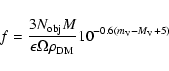 |
(11) |
where
 is the number of objects in the sample,
 is the local density
of halo dark matter, M is the average mass of the white dwarfs in
the HDF for a given simulation,
is the local density
of halo dark matter, M is the average mass of the white dwarfs in
the HDF for a given simulation,  is the apparent magnitude
cut of Ibata et al. (1999) as given in Table 4,
is the apparent magnitude
cut of Ibata et al. (1999) as given in Table 4,  is the
absolute magnitude of the dimmest white dwarf in the simulated sample,
is the
absolute magnitude of the dimmest white dwarf in the simulated sample,
 arcmin2 is the area surveyed by the HDF, and
  is the fraction of white dwarfs within the selection
criteria over the total number of white dwarfs. This fraction has
been estimated to be
is the fraction of white dwarfs within the selection
criteria over the total number of white dwarfs. This fraction has
been estimated to be
 (Ibata et al. 1999), but its
real value is uncertain. Consequently, this expression does not fully
take into account all the biases introduced by the selection process
and, hence, the adopted value of
can only be regarded as a
relatively bona fide estimate. Instead, the dark matter fraction has
been computed in the following way.
(Ibata et al. 1999), but its
real value is uncertain. Consequently, this expression does not fully
take into account all the biases introduced by the selection process
and, hence, the adopted value of
can only be regarded as a
relatively bona fide estimate. Instead, the dark matter fraction has
been computed in the following way.
![\begin{figure}
\par\includegraphics[width=8.8cm,clip]{0541fig07.ps}
\end{figure}](/articles/aa/full/2004/16/aa0541/Timg141.gif) |
Figure 7:
Simulation of the HDF. The box represents the observational
selection criteria of Ibata et al. (1999). |
| Open with DEXTER |
Table 5:
Summary of the results for the HDF obtained with our Monte
Carlo simulator for the different proposed IMFs.
The expected number of objects in the sample, is given by
 ,
where
,
where
 is the effective volume of the
sample and
is the effective volume of the
sample and
 .
As shown in Eq. (11) the usual way to
compute the effective volume of the sample is
.
As shown in Eq. (11) the usual way to
compute the effective volume of the sample is
 where d is taken to be
 .
Another, more accurate, way of
computing the effective volume is to use the
method as
it follows. For each star of the sample we determine the maximum
distance over which any star can contribute to the sample,
.
Another, more accurate, way of
computing the effective volume is to use the
method as
it follows. For each star of the sample we determine the maximum
distance over which any star can contribute to the sample,
and the minimum distance as well:
where  is the stellar parallax,
  its proper
motion, m the apparent magnitude,
its proper
motion, m the apparent magnitude,
 and
and
 are the low and high proper motion limits, if any, and
  and
and  are the corresponding magnitude limit. The maximum volume
in which a star can contribute is then
are the corresponding magnitude limit. The maximum volume
in which a star can contribute is then
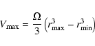
and the number density of white dwarfs will be

The effective volume of the sample can be then computed as:

The value of
is a measure of the
completeness of the sample, which is related to
by
We remind here that for a complete and homogeneous sample
 .
.
The results for the HDF simulations are also shown in Table 5. For
each of the cases we show the number of expected white dwarfs in the
HDF,
,
with its corresponding standard deviation, the
effective volume surveyed, the value of
,
the estimated completeness, the average distance of the
white dwarfs in the field, and the corresponding fraction of dark
matter derived from the simulations. An analysis of Table 5 reveals
that the expected number of objects is roughly 3 in all the cases
except for the case CSM2, for which the value of expected white dwarfs
is much larger. It is interesting to compare these values with the
expected number of objects if all the dark matter of the Galaxy were
in the form of white dwarfs. This number ranges, depending on the
selection criteria in colors and magnitudes, from 9 to 12. Clearly
even biased mass functions such as the AL and CSM1 mass functions are
not able to fill the halo with white dwarfs. Moreover, for the CSM2
case even if we adopt the lower limit of 24 objects in the field the
result is clearly much larger than that needed to fill all the halo
with white dwarfs.
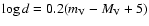
On the other hand, the effective volume surveyed by the HDF turns out
to be dependent of the adopted model IMF. This would not be the case
if Eq. (11) would have been adopted since in this case the effective
volume surveyed only depends on the absolute magnitude of the faintest
white dwarf in all the simulated samples which turns out to be
 - in accordance with the value adopted by Richer et al. (2000) - and on the adopted magnitude cut (
 ). It follows then that if this was the case, the radius of the
effective volume would be in all cases 2.2 kpc. The average
proper motions obtained are in all four cases very difficult to
measure: 26 mas yr-1, for the standard IMF, 30 mas yr-1 for the CSM1 case, 34 mas yr-1 for the
CSM2 mass function and 32 mas yr-1 for the AL case. The
typical standard deviation is
). It follows then that if this was the case, the radius of the
effective volume would be in all cases 2.2 kpc. The average
proper motions obtained are in all four cases very difficult to
measure: 26 mas yr-1, for the standard IMF, 30 mas yr-1 for the CSM1 case, 34 mas yr-1 for the
CSM2 mass function and 32 mas yr-1 for the AL case. The
typical standard deviation is  15 mas yr-1. It is important
to realize that these values are in agreement with the observed value
of
15 mas yr-1. It is important
to realize that these values are in agreement with the observed value
of  mas yr-1 (Ibata et al. 1999). The completeness of
the sample is roughly the same in all four cases, whereas for the
average distance of the microlenses we have significant variations. In
particular for the standard IMF the average distance is considerably
larger than in the rest of the simulations, being the case CSM2 an
extreme case. Finally, the fraction of baryonic dark matter in the
form of white dwarfs for the CSM2 case is totally incompatible with
the observations, whereas in the rest of the cases is significantly
smaller. For instance, for the case the CSM1 and AL mass functions
the fractions are comparable, and for the standard IMF the fraction of
baryonic dark matter only amounts to a modest 4%. Finally it is
worth noticing here that if we had used the selection criteria of
Flynn et al. (1996) we would have not found any white dwarf in the
HDF, whereas if we have used those of Méndez et al. (1996) we would
have found
mas yr-1 (Ibata et al. 1999). The completeness of
the sample is roughly the same in all four cases, whereas for the
average distance of the microlenses we have significant variations. In
particular for the standard IMF the average distance is considerably
larger than in the rest of the simulations, being the case CSM2 an
extreme case. Finally, the fraction of baryonic dark matter in the
form of white dwarfs for the CSM2 case is totally incompatible with
the observations, whereas in the rest of the cases is significantly
smaller. For instance, for the case the CSM1 and AL mass functions
the fractions are comparable, and for the standard IMF the fraction of
baryonic dark matter only amounts to a modest 4%. Finally it is
worth noticing here that if we had used the selection criteria of
Flynn et al. (1996) we would have not found any white dwarf in the
HDF, whereas if we have used those of Méndez et al. (1996) we would
have found  white dwarfs in HDF, almost independently of the
adopted IMF. Hence, it seems that a significant fraction of the
objects found by Méndez et al. (1996) should not be white dwarfs.
white dwarfs in HDF, almost independently of the
adopted IMF. Hence, it seems that a significant fraction of the
objects found by Méndez et al. (1996) should not be white dwarfs.
![\begin{figure}
\par\includegraphics[width=8.8cm,clip]{0541fig08.ps}
\end{figure}](/articles/aa/full/2004/16/aa0541/Timg166.gif) |
Figure 8:
Simulation of the EROS results. See text for a detailed
description. |
| Open with DEXTER |
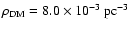
The EROS team has reported very recently (Goldman et al. 2002) the
results of a proper motion survey which aimed to discover faint halo
white dwarfs with high proper motions. However, they did not detect
any candidate halo white dwarf even if the survey was sensitive down
to
 and to proper motions as large as
 .
Moreover, they found that the
halo white dwarf contribution cannot exceed 5% at the 95% confidence
level for objects with color index
.
Moreover, they found that the
halo white dwarf contribution cannot exceed 5% at the 95% confidence
level for objects with color index
 .
It should
be noted however that this last result is dependent on the adopted
model of the Galaxy. In particular Goldman et al. (2002) adopted the
biased mass function CSM1 and in order to compare with the
observational results they only simulated white dwarfs with magnitudes
in the range
.
It should
be noted however that this last result is dependent on the adopted
model of the Galaxy. In particular Goldman et al. (2002) adopted the
biased mass function CSM1 and in order to compare with the
observational results they only simulated white dwarfs with magnitudes
in the range
 and color index within
 .
It is therefore necessary to extend the
study to other mass functions and, moreover, to the full range of
white dwarf magnitudes and colors. Additionally, since the results of
the EROS team are closely connected with those of the HDF studied in
Sect. 3.4 before, it is interesting to study the results obtained
with our Monte Carlo simulator.
.
It is therefore necessary to extend the
study to other mass functions and, moreover, to the full range of
white dwarf magnitudes and colors. Additionally, since the results of
the EROS team are closely connected with those of the HDF studied in
Sect. 3.4 before, it is interesting to study the results obtained
with our Monte Carlo simulator.
In Fig. 8 a typical Monte Carlo realization of the EROS results is
shown, whereas in Table 6 the average values for the ensemble of 40 independent realizations are also shown. The entries in Table 6 are
the same of Table 5, except for the distance which is expressed in
pc. The selection criteria of the EROS collaboration are shown as
dashed lines in Fig. 8. First, halo white dwarfs should have a
reduced proper motion
 ,
this restriction
is shown in Fig. 8 as a dashed diagonal line. Additionally they
required
,
this restriction
is shown in Fig. 8 as a dashed diagonal line. Additionally they
required
 .
Both limits are shown as well in Fig. 8 as a
horizontal dashed lines. As it can be seen in Table 6 and in Fig. 8, in the region where the EROS experiment conducted their search for
halo white dwarfs very few of them would be eventually found. In
particular for the case in which a standard mass function is used
only 2 of them (in the best of the cases) would be found. This is not the
case for the biased mass functions CSM1 and AL for which 6 white
dwarfs could be presumably found, whereas for the CSM2 case this
number increases to 12. Since the EROS experiment found none the only
mass function that seems to fit the observational data is the standard
one. In summary, both the results of the HDF, and of the EROS
experiment point towards the same conclusion: that the IMF adopted for
the halo should be the standard one.
.
Both limits are shown as well in Fig. 8 as a
horizontal dashed lines. As it can be seen in Table 6 and in Fig. 8, in the region where the EROS experiment conducted their search for
halo white dwarfs very few of them would be eventually found. In
particular for the case in which a standard mass function is used
only 2 of them (in the best of the cases) would be found. This is not the
case for the biased mass functions CSM1 and AL for which 6 white
dwarfs could be presumably found, whereas for the CSM2 case this
number increases to 12. Since the EROS experiment found none the only
mass function that seems to fit the observational data is the standard
one. In summary, both the results of the HDF, and of the EROS
experiment point towards the same conclusion: that the IMF adopted for
the halo should be the standard one.
Table 6:
Summary of the results for the EROS experiment obtained with
our Monte Carlo simulator for the different proposed IMFs.
![\begin{figure}
\par\includegraphics[width=8.4cm,clip]{0541fig09.ps}
\end{figure}](/articles/aa/full/2004/16/aa0541/Timg177.gif) |
Figure 9:
The halo white dwarf luminosity function obtained when
assuming that all the reported microlensing optical depth is
due to lenses in the form of white dwarfs - solid line -
compared to the observation luminosity functions of the disk
- top dotted line - and of the halo - bottom dotted line. |
| Open with DEXTER |
As it can be seen from Tables 2 and 3 our results are compatible with
a halo where roughly 10% of the dark matter is in the form of white
dwarfs. It is thus interesting to ask ourselves what would eventually
be the observed luminosity function of halo white dwarfs if all
the microlensing events (and the associated optical depth) are due to
halo white dwarfs. To this regard we have conducted a series of
simulations in which we have produced as many white dwarfs as needed
in order to reproduce the optical depth found by the MACHO team, which
roughly corresponds to  microlenses. In all these simulations
the standard IMF was adopted, since the biased mass functions AL and CSM1 studied in the previous sections produce roughly the same results
with regard to the white dwarf luminosity function. It is worth
noticing as well that the ad-hoc mass functions studied here
overproduce white dwarfs either in the HDF or in the EROS survey in
sharp contrast with the observations. The white dwarf luminosity
function was then computed using the restrictions for the visual
magnitude and proper motion detailed in Sect. 2.1. As was done in
Sect. 3.1, forty independent realizations of this sample were computed to
obtain the average white dwarf luminosity function along with its
corresponding standard deviation for each luminosity bin. The result
is shown in Fig. 9 as a solid line. For the sake of the comparison
the observational disk and halo white dwarf luminosity functions of
Bergeron et al. (1998) for the disk and of Torres et al.
(1998) for the halo are also shown as dotted lines. As it can be seen
in this figure, should white dwarfs be responsible of all the
microlensing events the halo white dwarf luminosity function would be
much closer to that of the disk rather than to that of the halo. It
is, however, worth mentioning at this point that this is indeed an
overestimate since for at least 4 lensing events it has been already
shown that the lenses are not in the Galactic halo. In particular,
one of the lenses resides in the galactic disk (Alcock et al. 2001a).
Moreover, three of these are binary events (Afonso et al. 1988; Bennet
et al. 1996; Alcock et al. 2001b) in the LMC or SMC. It is obvious,
that it is not possible that all lensing events with lenses in the LMC
and SMC are binary and, hence, it follows that a substantial fraction
of single events must also be in the LMC or the SMC as first pointed
out by Sahu (1994). However, it is true as well that this simulation
reinforces the result that most of the microlensing events reported by
the MACHO team are not halo white dwarfs and that another explanation
must be found for these results.
microlenses. In all these simulations
the standard IMF was adopted, since the biased mass functions AL and CSM1 studied in the previous sections produce roughly the same results
with regard to the white dwarf luminosity function. It is worth
noticing as well that the ad-hoc mass functions studied here
overproduce white dwarfs either in the HDF or in the EROS survey in
sharp contrast with the observations. The white dwarf luminosity
function was then computed using the restrictions for the visual
magnitude and proper motion detailed in Sect. 2.1. As was done in
Sect. 3.1, forty independent realizations of this sample were computed to
obtain the average white dwarf luminosity function along with its
corresponding standard deviation for each luminosity bin. The result
is shown in Fig. 9 as a solid line. For the sake of the comparison
the observational disk and halo white dwarf luminosity functions of
Bergeron et al. (1998) for the disk and of Torres et al.
(1998) for the halo are also shown as dotted lines. As it can be seen
in this figure, should white dwarfs be responsible of all the
microlensing events the halo white dwarf luminosity function would be
much closer to that of the disk rather than to that of the halo. It
is, however, worth mentioning at this point that this is indeed an
overestimate since for at least 4 lensing events it has been already
shown that the lenses are not in the Galactic halo. In particular,
one of the lenses resides in the galactic disk (Alcock et al. 2001a).
Moreover, three of these are binary events (Afonso et al. 1988; Bennet
et al. 1996; Alcock et al. 2001b) in the LMC or SMC. It is obvious,
that it is not possible that all lensing events with lenses in the LMC
and SMC are binary and, hence, it follows that a substantial fraction
of single events must also be in the LMC or the SMC as first pointed
out by Sahu (1994). However, it is true as well that this simulation
reinforces the result that most of the microlensing events reported by
the MACHO team are not halo white dwarfs and that another explanation
must be found for these results.
To check the sensitivity of our results with respect to a different
density profile we have done a final series of simulations in which
the density profile of Navarro et al. (1997) was adopted.
This density profile is characterized by the following expression
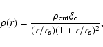 |
(12) |
where  is the scale radius,
 is
an adimensional characteristic density, and
is
an adimensional characteristic density, and
 is the critical density of an Einstein-De Sitter universe. On the
other hand,
is usually defined through the concentration
parameter
is the critical density of an Einstein-De Sitter universe. On the
other hand,
is usually defined through the concentration
parameter
 as a function of the virial radius,
R200. In order to correctly reproduce the rotation curve of our
Galaxy the following set of parameters is usually adopted: c=10,
R200=180 kpc, which results in
as a function of the virial radius,
R200. In order to correctly reproduce the rotation curve of our
Galaxy the following set of parameters is usually adopted: c=10,
R200=180 kpc, which results in
 kpc. In this
simulation, and as discussed previously, the adopted initial mass
function was the standard one. We only computed the number of
microlenses towards the LMC and not the results of the HDF or of
the EROS experiment.
kpc. In this
simulation, and as discussed previously, the adopted initial mass
function was the standard one. We only computed the number of
microlenses towards the LMC and not the results of the HDF or of
the EROS experiment.
![\begin{figure}
\par\includegraphics[width=7.8cm,clip]{0541fig10.ps}
\end{figure}](/articles/aa/full/2004/16/aa0541/Timg185.gif) |
Figure 10:
The density profiles used in the simulations. The top panel
shows the density profiles from the center of the Galaxy,
whereas the bottom panel shows the density profiles towards
the direction of the LMC. |
| Open with DEXTER |
The different density profiles used here are displayed in Fig. 10. The solid line corresponds to the classical isothermal sphere
density profile, the short dashed line to a power law with exponent
 ,
the long dashed line to a power law with
and the dashed-dotted line to the Navarro et al. (1997) density
profile. The top panel shows the density profile as a function of the
galactocentric r coordinate, whereas the bottom panel shows the
density profile projected towards the direction of the LMC. As it can
be seen in the top panel of Fig. 10, all the density profiles,
including that of Navarro et al. (1997), are much more concentrated
towards the center of the Galaxy than the isothermal sphere.
Additionally, the power law with
decreases much faster
than the other three density profiles considered here. However, when
projected towards the LMC, and for the distances of interest (those
relevant for the study of the microlenses towards the LMC, obtained in
the previous sections, 3 kpc), all four density profiles yield similar
densities. Consequently, we do not expect large departures from what
has been found in previous sections, and this is indeed the case. In
particular, the results obtained using the Navarro et al. (1997)
density profile are shown in Table 7, and it is evident from a cursory
inspection that the results do not differ much from those shown in
Table 3. Hence, the same conclusions apply, namely that the
contribution of halo white dwarfs to the microlensing events towards
the LMC must be small, independently of the adopted density profile.
,
the long dashed line to a power law with
and the dashed-dotted line to the Navarro et al. (1997) density
profile. The top panel shows the density profile as a function of the
galactocentric r coordinate, whereas the bottom panel shows the
density profile projected towards the direction of the LMC. As it can
be seen in the top panel of Fig. 10, all the density profiles,
including that of Navarro et al. (1997), are much more concentrated
towards the center of the Galaxy than the isothermal sphere.
Additionally, the power law with
decreases much faster
than the other three density profiles considered here. However, when
projected towards the LMC, and for the distances of interest (those
relevant for the study of the microlenses towards the LMC, obtained in
the previous sections, 3 kpc), all four density profiles yield similar
densities. Consequently, we do not expect large departures from what
has been found in previous sections, and this is indeed the case. In
particular, the results obtained using the Navarro et al. (1997)
density profile are shown in Table 7, and it is evident from a cursory
inspection that the results do not differ much from those shown in
Table 3. Hence, the same conclusions apply, namely that the
contribution of halo white dwarfs to the microlensing events towards
the LMC must be small, independently of the adopted density profile.
In order to check the robustness of our results we have conducted a
series of numerical experiments in which, firstly, the distance to the LMC was varied by a 10% and, secondly, the tangential velocity of the
resulting white dwarf population was also varied by a 10%. In all
the cases a standard IMF was used. The results are shown in Table 8. Our fiducial model is shown in Col. 3. The second column
corresponds to a model in which a distance of 45 kpc was adopted,
whereas the model in which a distance of 55 kpc was used is shown in
Col. 4. Columns 5 and 6 correspond, respectively, to the models in
which the tangential velocities were decreased (
 )
and
increased (
)
and
increased (
 )
artificially by a 10%. As can be seen
there, the differences in all the cases are relatively small. For
instance decreasing the distance to the LMC from 50 to 45 decreases
the contribution of white dwarfs to the observed microlensing optical
depth by 6%, whereas the model in which the contribution of white
dwarfs to the microlensing optical depth would be largest is that in
which the tangential velocities of all the white dwarfs have been
increased by 10%. In this case the contribution amounts to a 13%. Given all these considerations it seems unlikely that we could
have underestimated the contribution of white dwarfs to the observed
microlensing optical depth.
)
artificially by a 10%. As can be seen
there, the differences in all the cases are relatively small. For
instance decreasing the distance to the LMC from 50 to 45 decreases
the contribution of white dwarfs to the observed microlensing optical
depth by 6%, whereas the model in which the contribution of white
dwarfs to the microlensing optical depth would be largest is that in
which the tangential velocities of all the white dwarfs have been
increased by 10%. In this case the contribution amounts to a 13%. Given all these considerations it seems unlikely that we could
have underestimated the contribution of white dwarfs to the observed
microlensing optical depth.
Table 7:
Summary of the results obtained for the microlensing events
towards the LMC when the density profile of Navarro et al.
(1997) is adopted. See text for more details.
Table 8:
Summary of the results obtained for a limiting magnitude of
 and diferent values of the LMC
distance and the tangential velocity.
and diferent values of the LMC
distance and the tangential velocity.
Using a Monte Carlo code we have computed self-consistently and
simultaneously the theoretical expectations of the number of white
dwarfs for four different observational results, namely the reported
microlensing events towards the Large Magellanic Cloud (Alcock et al.
1997, 2000), the local halo white dwarf luminosity function (Torres et al. 1998), the results of the Hubble Deep Field (Ibata et al. 1999)
and the results of the EROS experiment (Goldman et al. 2002). Our
Monte Carlo simulator takes into account all the known observational
biases and uses a thorough description of the properties of the
Galactic halo. In our calculations we have simulated the halo white
dwarf population for several halo ages (12, 14 and 16 Gyr). We have
also used four different initial mass functions: a standard IMF (Scalo
1998), the two ad-hoc initial mass functions of Chabrier et al.
(1996), and the biased initial mass function of Adams & Laughlin
(1996) - see Table 1.
We have found that none but the standard IMF is able to reproduce
simultaneously the observations of the HDF, of the EROS experiment and
of the local halo white dwarf luminosity function. In particular, the
most extreme initial mass function of Chabrier et al. (1996) largely
overproduces white dwarfs for both the EROS survey and for the HDF.
More precisely, the EROS experiment in their survey did not find any
candidate white dwarf whereas our simulations show that if this was
the initial mass function of the halo they should have found around 12 white dwarfs. The same holds for the HDF, where a maximum of 4 white
dwarfs should have been found, whereas our simulations using this IMF
yield about 30 white dwarfs. Thus, this IMF is completely ruled out by
observations. Regarding the more conservative IMF of Chabrier et al.
(1996) our simulations predict  white dwarfs for the HDF and
 for the EROS survey. Therefore, although this IMF is
marginally compatible with the results of the HDF and with the local
white dwarf luminosity function, it turns out that is incompatible
with the results of the EROS survey. Since the Adams & Laughlin
(1996) initial mass function is very similar to the Chabrier et al. (1996) mass function the same conclusions apply to this IMF.
for the EROS survey. Therefore, although this IMF is
marginally compatible with the results of the HDF and with the local
white dwarf luminosity function, it turns out that is incompatible
with the results of the EROS survey. Since the Adams & Laughlin
(1996) initial mass function is very similar to the Chabrier et al. (1996) mass function the same conclusions apply to this IMF.
Regarding the microlensing events towards the LMC we have found that
white dwarfs at most could be responsible for 1 event for the
case in which the standard IMF is adopted. This number increases up to
5 events for the cases in which the "moderate'' log-normal
mass function of Chabrier et al. (1996) and of Adams & Laughlin
(1996) are used. The contribution of these events to the observed
optical depth  is, respectively,
 ,
0.2
and 0.3. Hence, even if ad-hoc initial mass functions are adopted the
total number of microlensing events produced by halo white dwarfs and
the corresponding optical depth found by the MACHO team cannot be
recovered when the observational biases and other constraints are
taken into account. Moreover, the average duration of the simulated
microlensing events for all the samples in which biased mass functions
were used is considerably smaller than the observed one. In summary,
the ad-hoc initial mass functions of Chabrier et al. (1996) and of
Adams & Laughlin (1996), which were tailored to fit the observations
of the MACHO team, fail to reproduce the rest of the observational
constraints and do not yield the required number of microlensing
events (and, thus, do not significantly contribute to the optical
depth). Consequently they should be disregarded until new (and
unlikely) evidence would eventually appear.
,
0.2
and 0.3. Hence, even if ad-hoc initial mass functions are adopted the
total number of microlensing events produced by halo white dwarfs and
the corresponding optical depth found by the MACHO team cannot be
recovered when the observational biases and other constraints are
taken into account. Moreover, the average duration of the simulated
microlensing events for all the samples in which biased mass functions
were used is considerably smaller than the observed one. In summary,
the ad-hoc initial mass functions of Chabrier et al. (1996) and of
Adams & Laughlin (1996), which were tailored to fit the observations
of the MACHO team, fail to reproduce the rest of the observational
constraints and do not yield the required number of microlensing
events (and, thus, do not significantly contribute to the optical
depth). Consequently they should be disregarded until new (and
unlikely) evidence would eventually appear.
We would like to emphasize at this point that all the above mentioned
results are almost completely independent of the adopted halo
age. Moreover, in order to check whether or not our results are
sensitive to the density profile of the halo, we have extended our
simulations using the density profile of Navarro et al. (1997). We
have found that the microlensing results are not sensitive to the
choice of the density profile because at the distances of interest all
the density profiles studied here are coincident.
In summary, our results strongly suggest that a sizeable fraction of
the dynamical mass in the halo of our Galaxy cannot be in the form of
old hydrogen-rich white dwarfs. More specifically, for the case in
which a standard initial mass function is adopted this fraction turns
out to be of the order of 4% if we trust the results of the HDF or as
low as 1% if the results of the EROS team are adopted. In any case
the percentage obtained here is well below the claim of the MACHO team
that 20% of the dark halo of the Galaxy is tied up in half-solar mass
stellar bodies (Alcock et al. 2000), since the constraints set by red
star counts (Flynn et al. 1996) discard the possibility of low-mass
main sequence stars. On the other hand our results are in excellent
agreement not only with the observations of the HDF and of the EROS
experiment but also with the theoretical estimates of Graff et al.
(1998), 
 ,
Flynn et al. (2001),
,
Flynn et al. (2001),  ,
and more recently
Goldman et al. (2002),
,
and more recently
Goldman et al. (2002),  ,
and Zhao (2002), .
Of
course, the real nature of the reported microlensing events remains
still a mystery.
,
and Zhao (2002), .
Of
course, the real nature of the reported microlensing events remains
still a mystery.
Acknowledgements
Part of this work was supported by the MCYT grants AYA04094-C03-01
and 02, by the MCYT/DAAD grant HA2000-0038, and by the CIRIT.
- Abia, C.,
Domínguez, I., Straniero, O., et al. 2001, ApJ, 557, 126 [NASA ADS] [CrossRef] (In the text)
- Adams, F. C., &
Laughlin, G. 1996, ApJ, 468, 686 [NASA ADS] [CrossRef] (In the text)
- Afonso, C., Alard,
C., Albert, J. N., et al. 1998, A&A, 337, L17 [NASA ADS]
- Alcock, C.,
Allsman, R. A., Axelrod, T. S., et al. 1996, ApJ, 461, 84 [NASA ADS] [CrossRef] (In the text)
- Alcock, C.,
Allsman, R. A., Alves, D., et al. 1997, ApJ, 486, 697 [NASA ADS] [CrossRef] (In the text)
- Alcock, C.,
Allsman, R. A., Alves, D. R., et al. 2000, ApJ, 542, 281 [NASA ADS] [CrossRef] (In the text)
- Alcock, C.,
Allsman, R. A., Alves, D. R., et al. 2001, Nature, 414, 617 [NASA ADS] [CrossRef] (In the text)
- Alcock, C.,
Allsman, R. A., Alves, D. R., et al. 2001, ApJ, 552, 259 [NASA ADS] [CrossRef]
- Bennett, D. P.,
Alcock, C., Allsman, R. A., et al. 1996, Nucl. Phys. Proc. Suppl.,
51B, 152 [NASA ADS]
- Bergeron, P.,
Leggett, S. K., & Ruiz, M. T. 1998, ApJ, 497, 294 [NASA ADS] [CrossRef]
- Binney, J., &
Tremaine, H. 1987, Galactic Dynamics (Princeton: Princeton Univ.
Press)
(In the text)
- Canal, R., Isern, J.,
& Ruiz-Lapuente, P. 1997, ApJ, 1997, 488 [NASA ADS], 35
(In the text)
- Chabrier, G.,
Ségretain, L., & Méra, D. 1996, ApJ, 468, L21 [NASA ADS] [CrossRef] (In the text)
- Dehnen, W., &
Binney, J. 1998, MNRAS, 298, 387 [NASA ADS] [CrossRef] (In the text)
-
Díaz-Pinto, A., García-Berro, E., Hernanz, M., Isern, J.,
& Mochkovitch, R. 1994, A&A, 282, 86 [NASA ADS]
- Flynn, C., Gould, A.,
& Bahcall, J. N. 1996, ApJ, 466, L55 [NASA ADS] [CrossRef] (In the text)
- Flynn, C.,
Sommer-Larsen, J., Fuchs, B., Graff, D. S., & Salim, S. 2001,
MNRAS, 322, 553 [NASA ADS] [CrossRef] (In the text)
- Flynn, C.,
Holopainen, J., & Holmberg, J. 2003, MNRAS, 339, 817 [NASA ADS] [CrossRef] (In the text)
- García-Berro,
E., Hernanz, M., Mochkovitch, R., & Isern, J. 1988, A&A,
193, 141 [NASA ADS]
- García-Berro,
E., Torres, S., Isern, J., & Burkert, A. 1999, MNRAS, 302,
173 [NASA ADS] [CrossRef] (In the text)
- Gibson, B. K.,
& Mould, J. R. 1997, ApJ, 482, 98 [NASA ADS] [CrossRef] (In the text)
- Goldman, B.,
Afonso, A., Alard, Ch., et al. 2002, A&A, 389, 69 [NASA ADS] [CrossRef] (In the text)
- Gould, A., Flynn, C.,
& Bahcall, J. N. 1998, ApJ, 499, 728 [NASA ADS] [CrossRef]
- Graff, D. S.,
Laughlin, G., & Freese, K. 1998, ApJ, 499, 7 [NASA ADS] [CrossRef] (In the text)
- Green, A. M., &
Jedamzik, K. 2002, A&A, 395, 31 [EDP Sciences] [NASA ADS] [CrossRef] (In the text)
- Gyuk, G., Dalal, N.,
& Griest, K. 2000, ApJ, 535, 90 [NASA ADS] [CrossRef] (In the text)
- Hansen, B. M. S.
1999, ApJ, 520, 680 [NASA ADS] [CrossRef] (In the text)
- Hernanz, M.,
García-Berro, E., Isern, J., et al. 1994, ApJ, 434, 652 [NASA ADS] [CrossRef] (In the text)
- Ibata, R. A., Richer,
H. B., Gilliland, R. L., & Scott, D. 1999, ApJ, 524, L95 [NASA ADS] [CrossRef] (In the text)
- Iben, I., &
Laughlin, G. 1989, ApJ, 341, 312 [NASA ADS] [CrossRef] (In the text)
- Isern, J.,
García-Berro, E., Hernanz, M., Mochkovitch, R., & Burkert,
A. 1995a, in White Dwarfs, ed. D. Koester, & K. Werner
(Heidelberg: Springer Verlag), 19
(In the text)
- Isern, J.,
García-Berro, E., Hernanz, M., Mochkovitch, R., & Burkert,
A. 1995b, in The Formation of the Milky Way, ed. E. J. Alfaro,
& A. J. Delgado (Cambridge: Cambridge University Press),
19
- Isern, J.,
García-Berro, E., Hernanz, M., Mochkovitch, R., & Torres,
S. 1998, ApJ, 503, 239 [NASA ADS] [CrossRef] (In the text)
- Isern, J.,
García-Berro, E., Hernanz, M., & Chabrier, G. 2000, ApJ,
528, 397 [NASA ADS] [CrossRef] (In the text)
- Knox, R. A., Hawkins,
M. R. S., & Hambly, N. C. 1999, MNRAS, 306, 736 [NASA ADS] [CrossRef] (In the text)
- James, F. 1990,
Comput. Phys. Commun., 60, 329 [NASA ADS] [MathSciNet] (In the text)
- Lasserre, T.,
Afonso, C., Albert, J. N., et al. 2001, A&A, 355, L39 [NASA ADS] (In the text)
- Leggett, S. K.,
Ruiz, M. T., & Bergeron, P. 1998, ApJ, 497, L294 [NASA ADS] [CrossRef] (In the text)
- Liebert, J.,
Dahn, C. C., & Monet, D. G. 1988, ApJ, 332, 891 [NASA ADS] [CrossRef] (In the text)
- Majewski, S.
R., & Siegel, M. H. 2002, ApJ, 569, 432 [NASA ADS] [CrossRef] (In the text)
- Markovic, D.,
& Sommer-Larsen, J. 1997, MNRAS, 288, 733 [NASA ADS]
- Méndez, R. A.,
Minnitti, D., De Marchi, G., Baker, A., & Couch, W. J. 1996,
MNRAS, 283, 666 [NASA ADS] (In the text)
- Navarro, J. F.,
Frenck, C. S., & White, S. D. M. 1997, ApJ, 490, 493 [NASA ADS] [CrossRef] (In the text)
- Nelson, C. A.,
Cook, K. H., Axelrod, T. S., Mould, J. R., & Alcock, C. 2002,
ApJ, 573, 644 [NASA ADS] (In the text)
- Noh, H.-R., & Scalo,
J. 1990, ApJ, 352, 605 [NASA ADS] [CrossRef] (In the text)
-
Oppenheimer, B. R., Hambly, N. C., Digby, A. P., Hodgkin, S. T.,
& Saumon, D. 2001, Science, 292, 698 [NASA ADS] [CrossRef]
- Oswalt, T. D.,
Smith, J. A., Wood, M. A., & Hintzen, P. 1996, Nature, 382,
692 [NASA ADS] [CrossRef] (In the text)
- Reylé, C.,
Robin, A. C., & Créze, M. 2001, A&A, L53
(In the text)
- Sahu, K. 1994, Nature, 370,
275 [NASA ADS] [CrossRef]
- Salati, P.,
Taillet, R., Aubourg, É., Palanque-Delabrouille, N., &
Spiro 1999, A&A, 350, L57 [NASA ADS] (In the text)
- Salaris, M.,
García-Berro, E., Hernanz, M., Isern, J., & Saumon, D.
2000, ApJ, 544, 1036 [NASA ADS] [CrossRef] (In the text)
- Scalo, J. 1998, in
The Stellar Initial Mass Function, ed. G. Gilmore, & D. Howell
(San Francisco), PASP Conf. Ser., 142, 201
(In the text)
- Schmidt, M. 1968,
ApJ, 151, 393 [NASA ADS] [CrossRef] (In the text)
- Torres, S.,
García-Berro, E., Burkert, A., & Isern, J. 2002, MNRAS,
333, 971 [NASA ADS] (In the text)
- Torres, S.,
García-Berro, E., & Isern, J. 1998, ApJ, 508, L71 [NASA ADS] [CrossRef] (In the text)
- Winget, D. E.,
Hansen, C. J., Liebert, J. G., et al. 1987, ApJ, 315, L77 [NASA ADS] [CrossRef] (In the text)
- Wu, X. 1994, ApJ, 435,
66 [NASA ADS] [CrossRef]
- Zhao, H. 2002, MNRAS,
336, 159 [NASA ADS] [CrossRef] (In the text)
Copyright ESO 2004
![\begin{figure}
\par\includegraphics[width=8.8cm,clip]{0541fig01.ps}
\end{figure}](/articles/aa/full/2004/16/aa0541/img75.gif)
![\begin{figure}
\par\includegraphics[width=8.8cm,clip]{0541fig02.ps}
\end{figure}](/articles/aa/full/2004/16/aa0541/img80.gif)
![\begin{figure}
\par\includegraphics[width=8.8cm,clip]{0541fig03.ps}
\end{figure}](/articles/aa/full/2004/16/aa0541/img90.gif)
![\begin{figure}
\par\includegraphics[width=8.8cm,clip]{0541fig04.ps}
\end{figure}](/articles/aa/full/2004/16/aa0541/img93.gif)
![\begin{figure}
\par\includegraphics[width=8.8cm,clip]{0541fig05.ps}
\end{figure}](/articles/aa/full/2004/16/aa0541/img121.gif)
![\begin{figure}
\par\includegraphics[width=8.8cm,clip]{0541fig06.ps}
\end{figure}](/articles/aa/full/2004/16/aa0541/img127.gif)
![\begin{figure}
\par\includegraphics[width=8.8cm,clip]{0541fig07.ps}
\end{figure}](/articles/aa/full/2004/16/aa0541/img141.gif)
![\begin{displaymath}r_{\rm max}={\rm min}\left[\pi^{-1}(\mu/\mu_{\rm l});~
\pi^{-1}10^{0.2(m_{\rm l}-m)}\right],\end{displaymath}](/articles/aa/full/2004/16/aa0541/img149.gif)
![\begin{displaymath}r_{\rm min}={\rm max}\left[\pi^{-1}(\mu/\mu_{\rm u});~
\pi^{-1}10^{0.2(m_{\rm u}-m)}\right],\end{displaymath}](/articles/aa/full/2004/16/aa0541/img150.gif)
![\begin{figure}
\par\includegraphics[width=8.8cm,clip]{0541fig08.ps}
\end{figure}](/articles/aa/full/2004/16/aa0541/img166.gif)
![\begin{figure}
\par\includegraphics[width=8.4cm,clip]{0541fig09.ps}
\end{figure}](/articles/aa/full/2004/16/aa0541/img177.gif)
![\begin{figure}
\par\includegraphics[width=7.8cm,clip]{0541fig10.ps}
\end{figure}](/articles/aa/full/2004/16/aa0541/img185.gif)