A&A 418, 363-369 (2004)
DOI: 10.1051/0004-6361:20034384
S. S. Tayal
Department of Physics, Clark Atlanta University, Atlanta, GA 30314, USA
Received 23 September 2003 / Accepted 7 November 2003
Abstract
The B-spline basis has been used in the R-matrix approach to calculate electron
impact excitation collision strengths for transitions between the
![]()
![]() ,
,
![]() and
and ![]() levels and from these levels to the fine-structure
levels of the excited
levels and from these levels to the fine-structure
levels of the excited
![]() ,
,
![]() ,
,
![]() ,
,
![]() and
and
![]() configurations of Cl II. We considered 23 LS states
configurations of Cl II. We considered 23 LS states
![]()
![]() ,
,
![]() ,
,
![]() ,
,
![]()
![]() ,
,
![]()
![]() ,
,
![]()
![]() ,
,
![]()
![]() ,
,
![]() ,
,
![]() ,
,
![]() ,
,
![]() ,
,
![]()
![]() ,
,
![]()
![]() ,
,
![]()
![]() ,
,
![]()
![]() ,
,
![]() and
and
![]()
![]() in the close-coupling expansion
that give rise to 51 fine-structure levels. The non-orthogonal orbitals are used for an
accurate representation of both the target wavefunctions and the R-matrix basis functions.
The collision strengths for transitions between fine-structure levels are calculated by
transforming the LS-coupled K-matrices to K-matrices in an intermediate coupling scheme.
The Rydberg series of resonances converging to excited state thresholds make substantial
contributions to collision strengths. The thermally averaged collision strengths have been
obtained by integrating collision strengths over a Maxwellian distribution of electron
energies and these are listed in Table 2 for log T from 3.3 to 5.6 K.
in the close-coupling expansion
that give rise to 51 fine-structure levels. The non-orthogonal orbitals are used for an
accurate representation of both the target wavefunctions and the R-matrix basis functions.
The collision strengths for transitions between fine-structure levels are calculated by
transforming the LS-coupled K-matrices to K-matrices in an intermediate coupling scheme.
The Rydberg series of resonances converging to excited state thresholds make substantial
contributions to collision strengths. The thermally averaged collision strengths have been
obtained by integrating collision strengths over a Maxwellian distribution of electron
energies and these are listed in Table 2 for log T from 3.3 to 5.6 K.
Key words: atomic data - atomic processes - line: formation
The fine-structure transitions among the levels of ground
![]() configuration in Cl II
give rise to spectral lines in the infrared and visible part of the spectrum and transitions
from the ground configuration to excited
configuration in Cl II
give rise to spectral lines in the infrared and visible part of the spectrum and transitions
from the ground configuration to excited
![]() ,
,
![]() ,
,
![]() ,
,
![]() and
and
![]() configurations occur in the ultraviolet (UV), far-ultraviolet (FUV) and
extreme ultraviolet (EUV) wavelength regions. Emission lines of collisionally excited Cl II
have been detected in the spectra of the Io torus from the ground-based observations
(Küppers & Schneider 2000) as well as from the space-based observations by the
Far-Ultraviolet Spectroscopic Explorer (FUSE) (Feldman et al. 2001). Electron-ion
collision processes play an important role in the understanding of energy balance in various
types of plasmas. Accurate electron impact collision strengths of fine-structure transitions
in Cl II are needed for the interpretation of observed spectra to understand the physical
processes and conditions such as temperature, density and chlorine abundance in Io-torus-Jupiter
system.
configurations occur in the ultraviolet (UV), far-ultraviolet (FUV) and
extreme ultraviolet (EUV) wavelength regions. Emission lines of collisionally excited Cl II
have been detected in the spectra of the Io torus from the ground-based observations
(Küppers & Schneider 2000) as well as from the space-based observations by the
Far-Ultraviolet Spectroscopic Explorer (FUSE) (Feldman et al. 2001). Electron-ion
collision processes play an important role in the understanding of energy balance in various
types of plasmas. Accurate electron impact collision strengths of fine-structure transitions
in Cl II are needed for the interpretation of observed spectra to understand the physical
processes and conditions such as temperature, density and chlorine abundance in Io-torus-Jupiter
system.
The strong mixing between a number of levels of the different Rydberg
![]() nl series
and the
nl series
and the
![]() perturber states are caused by configuration-interaction (Tayal 2003).
The Cl II wavefunctions show strong term dependence of the one-electron orbitals and large
correlation corrections. The term dependent non-orthogonal orbitals in the
multiconfiguration
Hartree-Fock approach (Froese Fischer 1991; Zatsarinny & Froese
Fischer 1999) have been used
to provide adequate treatment of large correlation corrections as well as the interactions
between different Rydberg series and perturber states. These wavefunctions yield excitation
energies of Cl II target states that are in excellent agreement with the experimental values.
The B-spline R-matrix approach (Zatsarinny & Froese Fischer 1999;
Zatsarinny & Tayal 2001)
has been used to calculate electron impact excitation collision strengths and effective
collision strengths for all dipole allowed, intercombination and forbidden transitions among
the fine-structure levels. Our calculation included 23 spectroscopic bound states of Cl II in
the close-coupling expansion. We included 15 states
perturber states are caused by configuration-interaction (Tayal 2003).
The Cl II wavefunctions show strong term dependence of the one-electron orbitals and large
correlation corrections. The term dependent non-orthogonal orbitals in the
multiconfiguration
Hartree-Fock approach (Froese Fischer 1991; Zatsarinny & Froese
Fischer 1999) have been used
to provide adequate treatment of large correlation corrections as well as the interactions
between different Rydberg series and perturber states. These wavefunctions yield excitation
energies of Cl II target states that are in excellent agreement with the experimental values.
The B-spline R-matrix approach (Zatsarinny & Froese Fischer 1999;
Zatsarinny & Tayal 2001)
has been used to calculate electron impact excitation collision strengths and effective
collision strengths for all dipole allowed, intercombination and forbidden transitions among
the fine-structure levels. Our calculation included 23 spectroscopic bound states of Cl II in
the close-coupling expansion. We included 15 states
![]()
![]() ,
,
![]() ,
,
![]() ,
,
![]()
![]() ,
,
![]()
![]() ,
,
![]()
![]() ,
,
![]()
![]() ,
,
![]() ,
,
![]() ,
,
![]()
![]() ,
,
![]()
![]() and
eight higher-lying states
and
eight higher-lying states
![]()
![]() ,
,
![]()
![]() ,
,
![]() ,
,
![]() ,
,
![]()
![]() ,
,
![]() ,
,
![]()
![]() which have strong
dipole connection with the
which have strong
dipole connection with the
![]() terms. A B-spline basis has been used for the description of
continuum functions. No orthogonality constraint has been imposed on the continuum functions and
atomic bound orbitals. This procedure leads to substantial reduction in pseudo-resonances in the
electron collisional excitation strengths. The completeness of the B-spline ensures that no Buttle
correction to the R-matrix elements is required.
terms. A B-spline basis has been used for the description of
continuum functions. No orthogonality constraint has been imposed on the continuum functions and
atomic bound orbitals. This procedure leads to substantial reduction in pseudo-resonances in the
electron collisional excitation strengths. The completeness of the B-spline ensures that no Buttle
correction to the R-matrix elements is required.
Recently, Wilson & Bell (2002) reported collision data for the 10 fine-structure transitions
among the ground configuration levels
![]()
![]() ,
,
![]() and
and ![]() of Cl II.
They included lowest 12 LS states
of Cl II.
They included lowest 12 LS states
![]()
![]() ,
,
![]() ,
,
![]() ,
,
![]()
![]() ,
,
![]()
![]() ,
,
![]()
![]() ,
,
![]()
![]() ,
,
![]() ,
,
![]() and
and
![]()
![]() in the close-coupling expansion in their R-matrix calculations and used
configuration-interaction (CI) wavefunctions (Hibbert 1975) for these target states that
were constructed with eight spectroscopic 1s, 2s, 2p, 3s, 3p, 3d, 4s and 4p orbitals and two
pseudo-orbitals 4d and 4f. Earlier, a theoretical calculation of electron impact excitation of Cl II
was reported by Krueger & Czyzak (1970) using a distorted wave approximation and
using Hartree-Fock (HF) representation of Cl II target states. Berrington & Nakazaki (2002)
reported bound state energies, oscillator strengths and ground state photoionization
cross sections for chlorine and its ions. Tayal (2003) investigated the term dependence
of wavefunctions, interactions between the different
in the close-coupling expansion in their R-matrix calculations and used
configuration-interaction (CI) wavefunctions (Hibbert 1975) for these target states that
were constructed with eight spectroscopic 1s, 2s, 2p, 3s, 3p, 3d, 4s and 4p orbitals and two
pseudo-orbitals 4d and 4f. Earlier, a theoretical calculation of electron impact excitation of Cl II
was reported by Krueger & Czyzak (1970) using a distorted wave approximation and
using Hartree-Fock (HF) representation of Cl II target states. Berrington & Nakazaki (2002)
reported bound state energies, oscillator strengths and ground state photoionization
cross sections for chlorine and its ions. Tayal (2003) investigated the term dependence
of wavefunctions, interactions between the different
![]() ,
,
![]() and
and
![]() Rydberg series and
importance of correlation corrections in Cl II using the non-orthogonal orbitals.
Rydberg series and
importance of correlation corrections in Cl II using the non-orthogonal orbitals.
Accurate representation of target wavefunctions is an essential ingredient of a reliable collision
calculation. The target states in our calculation are accurately represented by non-orthogonal
orbitals obtained by separate optimization of each target state. The non-orthogonal orbitals allow
to include correlation corrections with a minimum number of configurations and correlated orbitals.
However, non-orthogonal orbitals technique is computationally more time consuming than the orthogonal
orbitals. Earlier calculation of Cl II wavefunctions by Wilson & Bell (2002) used
the same set of orthogonal orbitals. They included a pseudo-orbital 4d to account for the term dependence
of 3d orbital and a pseudo-orbital 4f to include correlation corrections. In our calculation we used
non-orthogonal orbitals for the description of term-dependence of radial functions. The 3s and 3p
orbitals in the
![]() and
and
![]() configurations are similar, but differ in the
configurations are similar, but differ in the
![]() and
and
![]() nl configurations. We used two different sets of 3s and 3p orbitals; one for the
nl configurations. We used two different sets of 3s and 3p orbitals; one for the
![]() and
and
![]() configurations and another for the
configurations and another for the
![]() nl configurations.
Different valence 4s, 4p,
3d and 4d orbitals are obtained for the individual
nl configurations.
Different valence 4s, 4p,
3d and 4d orbitals are obtained for the individual
![]() nl 1,3,5L(L = 0, 1, 2, 3) states in separate calculations. Additional to spectroscopic orbitals we obtained several
s, p, d and f correlation orbitals to account for core correlation, core-polarization or core-valence
correlation and interactions between different Rydberg series. The mean radii of the correlation
orbitals are comparable to the 3s, 3p, 3d, 4s and 4p spectroscopic orbitals and thus represent the
correlation corrections very well. We found that the core-valence correlation where one electron from
the 3s subshell of the
nl 1,3,5L(L = 0, 1, 2, 3) states in separate calculations. Additional to spectroscopic orbitals we obtained several
s, p, d and f correlation orbitals to account for core correlation, core-polarization or core-valence
correlation and interactions between different Rydberg series. The mean radii of the correlation
orbitals are comparable to the 3s, 3p, 3d, 4s and 4p spectroscopic orbitals and thus represent the
correlation corrections very well. We found that the core-valence correlation where one electron from
the 3s subshell of the
![]() core is excited to the outer orbitals and core correlation
core is excited to the outer orbitals and core correlation
![]() represent large correlation corrections.
represent large correlation corrections.
The wave function describing the total (N+1)-electron system in the
internal region surrounding the atom with radius ![]() is expanded in
terms of energy-independent functions (Berrington et al. 1995)
is expanded in
terms of energy-independent functions (Berrington et al. 1995)
 |
(1) |
The LS-coupled K-matrices are calculated by matching the inner region solutions at r = a with asymptotic solutions in the outer region. The FARM program (Burke & Noble 1995) has been used to find the asymptotic solutions. The collision strengths between fine-structure levels are calculated by transforming the LS-coupled K-matrices to K-matrices in an intermediate coupling scheme. We have used the intermediate-coupling frame transformation (ICFT) method (Giffin et al. 1998). This method employs multi-channel quantum defect theory (MQDT) to generate unphysical K-matrices in LS coupling and these are transformed to intermediate coupling. The physical K-matrices are then obtained from the intermediate-coupled unphysical K-matrices. The higher partial wave contributions for the dipole-allowed and other transitions are calculated using a top-up procedure based on the geometric series approximation (Burgess et al. 1970).
In the asymptotic region,
the collision strength follows a high energy limiting behavior
which is determined by the type of transition. For optically
allowed electric-dipole transitions
| (3) |
| (4) |
| (5) |
In many applications it is convenient to use excitation rate coefficients or
thermally averaged collision strengths as a function of electron temperature.
The electron excitation rates are obtained by averaging total collision
strengths over a Maxwellian distribution of electron energies. The
excitation rate coefficient for a transition from state i to state fat electron temperature ![]() is given by
is given by
 |
(6) |
 |
(7) |
The effective collision strengths are calculated by integrating collision strengths for fine-structure levels over a Maxwellian distribution of electron energies.
![\begin{figure}
\par\includegraphics[angle=-90,width=15cm,clip]{0384fig1.eps} \end{figure}](/articles/aa/full/2004/16/aa0384/img57.gif) |
Figure 1:
Collision strength for the forbidden
|
| Open with DEXTER | |
![\begin{figure}
\par\includegraphics[angle=-90,width=15cm,clip]{0384fig2.eps} \end{figure}](/articles/aa/full/2004/16/aa0384/img58.gif) |
Figure 2:
Collision strength for the forbidden
|
| Open with DEXTER | |
Table 1: Excitation energies of Cl II states relative to the ground state. Present theory is compared with the NIST compilation (http://physics.nist.gov) and the calculations of Wilson & Bell (2002) (WB) and Berrington & Nakazaki (2002) (BN).
Our target wavefunctions correctly represent the main correlation corrections and the interaction between different Rydberg series and perturbers as indicated by excellent agreement between the calculated excitation energies and experimental values. Excitation energies of the 23 LS Cl II target states relative to the ground state are presented in Table 1 where our calculated results are compared with the experimental values from the National Institute of Standard and Technology (NIST) (http://physics.nist.gov) and the calculations of Wilson & Bell (2002) and Berrington & Nakazaki (2002). Wilson & Bell (2002) calculated wavefunctions for the 12 LS Cl II states and Berrington & Nakazaki (2002) used R-matrix method (Berrington et al. 1995) to obtain radiative data for a large number of Cl II terms. Our calculation shows very good agreement with the calculation of Berrington & Nakazaki (2002) except for the assignments of the lowest
![\begin{figure}
\par\includegraphics[angle=-90,width=16cm,clip]{0384fig3.eps} \end{figure}](/articles/aa/full/2004/16/aa0384/img64.gif) |
Figure 3:
Collision strength for the forbidden
|
| Open with DEXTER | |
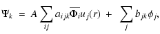
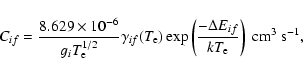
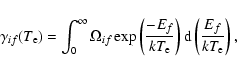
We chose a fine energy mesh (0.0002 Ryd) for collision strengths calculation in the thresholds
energy region which allowed us to include resonance structures accurately. We calculated collision
strengths at 8150 energy points in the thresholds region upto 1.60 Ryd and at 150 energy points in
the above threshold region upto 16.6 Ryd. The collision strengths are displayed as a function
of electron energy for the low-lying forbidden
![]()
![]() -
-
![]()
![]() ,
,
![]()
![]() -
-
![]()
![]() and
and
![]()
![]() -
-
![]()
![]() transitions
in Figs. 1-3 respectively
in the thresholds energy region. Our results can be compared with 12-state
R-matrix calculation of Wilson & Bell (2002) (not shown). Both calculations exhibit
similar complicated resonance structure because of the interference and overlapping of several Rydberg
series of resonances. Our calculation includes additional resonances converging to higher excited states
above 1.15 Ryd because of the inclusion of additional 11 target states in the close-coupling expansion
in our work that have thresholds between 1.172 Ryd and 1.598 Ryd. It is clear that these resonances
converging to higher excited states make significant contributions.
There seem to be some differences in
the background collision strengths away from resonances from the
two calculations. These differences
can be clearly noted for the
transitions
in Figs. 1-3 respectively
in the thresholds energy region. Our results can be compared with 12-state
R-matrix calculation of Wilson & Bell (2002) (not shown). Both calculations exhibit
similar complicated resonance structure because of the interference and overlapping of several Rydberg
series of resonances. Our calculation includes additional resonances converging to higher excited states
above 1.15 Ryd because of the inclusion of additional 11 target states in the close-coupling expansion
in our work that have thresholds between 1.172 Ryd and 1.598 Ryd. It is clear that these resonances
converging to higher excited states make significant contributions.
There seem to be some differences in
the background collision strengths away from resonances from the
two calculations. These differences
can be clearly noted for the
![]()
![]() -
-
![]()
![]() transition shown in Fig. 3 of the
present paper and Fig. 10 of their paper. The differences in background collision strengths are perhaps
caused by the differences in the wavefunctions used in the two calculations.
transition shown in Fig. 3 of the
present paper and Fig. 10 of their paper. The differences in background collision strengths are perhaps
caused by the differences in the wavefunctions used in the two calculations.
We have plotted collision strengths as a function of electron energy in the above highest excitation
threshold region from 1.6 Ryd to 16.6 Ryd in Fig. 4 for the allowed
![]()
![]() -
-
![]()
![]() (solid curve),
(solid curve),
![]()
![]() -
-
![]()
![]() (long-dashed curve) and
(long-dashed curve) and
![]()
![]() -
-
![]()
![]() (short-dashed curve) transitions. The collision
strengths in this energy region show smooth variation with energy. The collision strengths for allowed
transitions show increasing trend with energy in the high energy region and depend on the oscillator
strength of the transitions (Eq. (3)). It is clear from Fig. 4 that the
(short-dashed curve) transitions. The collision
strengths in this energy region show smooth variation with energy. The collision strengths for allowed
transitions show increasing trend with energy in the high energy region and depend on the oscillator
strength of the transitions (Eq. (3)). It is clear from Fig. 4 that the
![]()
![]() -
-
![]()
![]() transition is the strongest of the three allowed transitions.
transition is the strongest of the three allowed transitions.
![\begin{figure}
\par\includegraphics[angle=-90,width=8.8cm,clip]{0384fig4.eps} \end{figure}](/articles/aa/full/2004/16/aa0384/img65.gif) |
Figure 4:
Collision strength for the allowed
|
| Open with DEXTER | |
The effective collision strengths are calculated by taking into account important resonance effects.
These are obtained by integrating resonant collision strengths below the highest excitation threshold
and smooth collision strengths above the highest threshold over a Maxwellian distribution of electron
energies (Eq. (7)). In Table 2 we present effective collision strengths for all transitions between the
![]()
![]() ,
,
![]() and
and ![]() levels and from these levels to the 38 fine-structure
levels of the excited configurations at electron temperatures from log T = 3.3 to 6.0 K.
The experimental
wavelengths of transitions are also listed in Table 2. For many
transitions the resonance effects in
collision strengths enhance the effective collision strengths substantially in the lower temperature
region. It may be noted that we presented effective collision strengths for 43 fine-structure levels
because the results for higher excitation levels (44-51) may not be accurate. The transitions involving
these higher excitation levels are less accurate because of the neglect of coupling to levels that
lie below and above. The main purpose of these levels in our calculation is to account for their strong
coupling with lower levels.
levels and from these levels to the 38 fine-structure
levels of the excited configurations at electron temperatures from log T = 3.3 to 6.0 K.
The experimental
wavelengths of transitions are also listed in Table 2. For many
transitions the resonance effects in
collision strengths enhance the effective collision strengths substantially in the lower temperature
region. It may be noted that we presented effective collision strengths for 43 fine-structure levels
because the results for higher excitation levels (44-51) may not be accurate. The transitions involving
these higher excitation levels are less accurate because of the neglect of coupling to levels that
lie below and above. The main purpose of these levels in our calculation is to account for their strong
coupling with lower levels.
![\begin{figure}
\par\includegraphics[angle=-90,width=8.8cm,clip]{0384fig5.eps} \end{figure}](/articles/aa/full/2004/16/aa0384/img66.gif) |
Figure 5:
Effective collision strength for the forbidden
|
| Open with DEXTER | |
![\begin{figure}
\par\includegraphics[angle=-90,width=8.8cm,clip]{0384fig6.eps} \end{figure}](/articles/aa/full/2004/16/aa0384/img67.gif) |
Figure 6:
Effective collision strength for the forbidden
|
| Open with DEXTER | |
![\begin{figure}
\par\includegraphics[angle=-90,width=8.8cm,clip]{0384fig7.eps} \end{figure}](/articles/aa/full/2004/16/aa0384/img69.gif) |
Figure 7:
Effective collision strength for the forbidden
|
| Open with DEXTER | |
![\begin{figure}
\par\includegraphics[angle=-90,width=8.8cm,clip]{0384fig8.eps} \end{figure}](/articles/aa/full/2004/16/aa0384/img70.gif) |
Figure 8:
Effective collision strength for the forbidden
|
| Open with DEXTER | |
We have presented elaborate calculations of collision strengths and effective collision strengths
for transitions between the
![]()
![]() ,
,
![]() and
and ![]() levels and from these
levels to 38 excited levels of Cl II. Our results are presented over a wide electron temperature
range suitable for use in astrophysical plasma modeling. In our work we used non-orthogonal orbitals
both for the representation of target wavefunctions and for the representation of scattering
functions. The use of non-orthogonal orbitals considerably simplifies the structure of the bound
part of the close-coupling expansion, that leads to substantial reduction in pseudo-resonances.
We used ICFT method to transform LS-coupled K-matrices to K-matrices in intermediate coupling.
This method should lead to improved accuracy compared to standard transformation method used by
Wilson & Bell (2002) to calculate level-to-level electron impact excitation collision strengths.
Our calculation should also be accurate because of the inclusion of additional 11 excited states
in the close-coupling expansion to ensure convergence of results for fine-structure transitions
presented in our work. Significant differences with earlier calculation (Wilson
& Bell 2002) are noted
for some transitions which may have important consequences for astrophysical plasma diagnostics.
levels and from these
levels to 38 excited levels of Cl II. Our results are presented over a wide electron temperature
range suitable for use in astrophysical plasma modeling. In our work we used non-orthogonal orbitals
both for the representation of target wavefunctions and for the representation of scattering
functions. The use of non-orthogonal orbitals considerably simplifies the structure of the bound
part of the close-coupling expansion, that leads to substantial reduction in pseudo-resonances.
We used ICFT method to transform LS-coupled K-matrices to K-matrices in intermediate coupling.
This method should lead to improved accuracy compared to standard transformation method used by
Wilson & Bell (2002) to calculate level-to-level electron impact excitation collision strengths.
Our calculation should also be accurate because of the inclusion of additional 11 excited states
in the close-coupling expansion to ensure convergence of results for fine-structure transitions
presented in our work. Significant differences with earlier calculation (Wilson
& Bell 2002) are noted
for some transitions which may have important consequences for astrophysical plasma diagnostics.
Acknowledgements
This research work was supported by NASA grant NAG5-13340 from the Planetary Atmospheres Program.