A. Amblard 1,4 - J.-Ch. Hamilton 1,2,3
1 - Physique Corpusculaire et Cosmologie, Collège de France, 11 pl. Marcelin Berthelot, 75231 Paris Cedex 05, France
2 -
Laboratoire de Physique Nucléaire et de Hautes Energies, 4, Place Jussieu, Tour 33, 75252
Paris Cedex 05, France
3 -
Laboratoire de Physique Subatomique et de Cosmologie, 53 Avenue des Martyrs, 38026 Grenoble Cedex, France
4 -
University of California, Department of Astronomy, 601 Campbell Hall, Berkeley, CA 94720-3411, USA
Received 10 July 2003 / Accepted 27 December 2003
Abstract
We present a method designed to estimate the noise power spectrum in the time domain for CMB experiments. The noise power spectrum is extracted from the time ordered data avoiding the
contamination coming from sky signal and accounting the pixellisation of the signal and the projection of the noise when making intermediate sky projections. This method is simple to
implement and relies on Monte-Carlo simulations, it runs on a simple desk computer. We also propose a trick for filtering data before making coadded maps in order to avoid ringing due to the presence of signal in the timelines. These algorithms were succesfully tested on Archeops data.
Key words: cosmic microwave background - cosmology: observations - large-scale structure of the Universe - methods: numerical
Measuring the Cosmic Microwave Background anisotropies angular power spectrum has proved to be a powerful cosmological tool giving direct information on both the cosmological parameters and the primordial Universe through the origin of the initial perturbations.
The usual method used nowadays for measuring the CMB temperature fluctuations is to scan the sky with a detector (with a bolometer for instance) that measures the temperature variations in a given beam. This provides time data streams along with pointing directions that are subsequently compressed into a sky map. In the general case, the noise in the time streams is not white (due to atmospheric contamination, spurious noises, electronic and detector temperature fluctuations). The sky is also in general not regularly scanned so that at the end, the noise in the maps is neither homogeneous nor white.
This causes difficulties when trying to extract the signal power spectrum from the maps as it has to be separated from the noise. Fully optimal methods finding the maximum likelihood solution for both the map and the CMB power spectrum have been proposed such as MADCAP (Borrill 1999) but they require the inversion of large covariance matrices on parallel supercomputers and are hard to implement for the present generation of experiments that cover a large portion of the sky and have a large number of pixels (WMAP, Archeops and Planck in the near future). Alternative methods that replace the full inversion by a Monte-Carlo simulation of the noise angular power spectrum have been proposed (Hivon et al. 2002; Szapudi et al. 2001). The results obtained with such methods are satisfactory and they consume little time compared to the maximum likelihood methods. The analysis process is done in the following way in these Monte-Carlo methods:
We present in this section the method we developed for determining the noise Fourier power spectrum of a time data stream composed of CMB fluctuations, some strong astrophysical foreground (here the Galactic dust emission) and coloured
Gaussian and stationary noise. The data is denoted as an N elements vector ![]() (N is the number of time samples) and is composed of noise
(N is the number of time samples) and is composed of noise ![]() and sky signal
and sky signal ![]() :
:
The first raw estimation of the noise power can come from the data itself (that is
![]() )
as we are dealing with low signal to noise experiments (at least in the time domain as the noise is reduced by redundancy in the map). This is a correct approximation
only in the case where the observed region of the sky is free from any
bright source. In most recent experiments such as WMAP and Archeops
(as well as in Planck) the instrument covers a large portion of the
sky by making large circles that often cross the Galactic plane twice per
rotation. There is therefore a very bright source in all the portions
of the time streams that prevent us from using the naive approximation
)
as we are dealing with low signal to noise experiments (at least in the time domain as the noise is reduced by redundancy in the map). This is a correct approximation
only in the case where the observed region of the sky is free from any
bright source. In most recent experiments such as WMAP and Archeops
(as well as in Planck) the instrument covers a large portion of the
sky by making large circles that often cross the Galactic plane twice per
rotation. There is therefore a very bright source in all the portions
of the time streams that prevent us from using the naive approximation
![]() .
.
Prior to any treatment we apply a high pass filter at
![]() (in our example 0.3 Hz), estimating the noise power spectrum only at frequencies higher than
(in our example 0.3 Hz), estimating the noise power spectrum only at frequencies higher than
![]() ,
from now
,
from now ![]() will therefore refer to the filtered data. This
will therefore refer to the filtered data. This
![]() corresponds to the frequency where the non-astrophysical foreground or
systematic (such as atmospheric emission) become negligible and where the low frequency
noise is not too strong (in the 1/f noise model that would roughly
corresponds to
corresponds to the frequency where the non-astrophysical foreground or
systematic (such as atmospheric emission) become negligible and where the low frequency
noise is not too strong (in the 1/f noise model that would roughly
corresponds to
![]() ).
).
A simple method to get rid of the signal contribution in the noise
power spectrum estimation is to project the data onto a map of the sky
portion observed. In such a map, the noise level is reduced
but the signal is almost unchanged. Reading back this map with the
scanning strategy leads to a timeline where the signal to noise is
greatly improved. This latter timeline can then be subtracted
from the initial timeline giving a noise estimate that is, in
principle, free from signal contamination. In the matrix notation
that has become common in CMB analysis this corresponds to the
following operation:
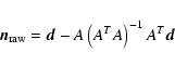
If one rewrites Eq. (2) using the definition (1), one gets:
![$\displaystyle %
\begin{array}{ccccccc}
\vec{n}_{{\rm raw}}&=&\vec{n}&-&\underbr...
...{s}\right)}\\ [4mm]
&=&\vec{n}&-&\vec{r}_{\rm n}&+&\vec{r}_{\rm s}
\end{array}$](/articles/aa/full/2004/15/aa0066/img17.gif) |
(3) |
If one can determine the shape of both
![]() and
and
![]() ,
then debiasing the noise power is straighforward by inverting Eq. (6).
,
then debiasing the noise power is straighforward by inverting Eq. (6).
The simplest way to estimate
![]() is to make noise only Monte-Carlo realizations of data streams with spectrum
is to make noise only Monte-Carlo realizations of data streams with spectrum
![]() (this assumes that
(this assumes that
![]() is close enough to P so that
is close enough to P so that ![]() is computed with enough accuracy although the algorithm could be iterated) and perform the operation of Eq. (2) on each realisation. The average power spectrum of all realizations is biased by
is computed with enough accuracy although the algorithm could be iterated) and perform the operation of Eq. (2) on each realisation. The average power spectrum of all realizations is biased by
![]() that can be calculated by taking the ratio of the input power spectrum to the output. The result obtained is shown in Fig. 1.
Large oscillations can be seen at lower frequencies with peaks at harmonics of the spinning frequency (0.035 Hz in our Archeops-like case). This is not surprising as we expect the noise
to project onto the sky at these frequencies. It is therefore at these particular frequencies that the noise bias is the largest, leading to large values of
that can be calculated by taking the ratio of the input power spectrum to the output. The result obtained is shown in Fig. 1.
Large oscillations can be seen at lower frequencies with peaks at harmonics of the spinning frequency (0.035 Hz in our Archeops-like case). This is not surprising as we expect the noise
to project onto the sky at these frequencies. It is therefore at these particular frequencies that the noise bias is the largest, leading to large values of
![]() .
The noise bias
transformed into harmonic power spectrum using the Archeops pointing strategy is shown in Fig. 2, showing that this effect should not be neglected as it amounts to a significant fraction of the error bars (shown in black in Fig. 6).
.
The noise bias
transformed into harmonic power spectrum using the Archeops pointing strategy is shown in Fig. 2, showing that this effect should not be neglected as it amounts to a significant fraction of the error bars (shown in black in Fig. 6).
![\begin{figure}
\par\includegraphics[width=7.8cm,clip]{0066fig1.ps}\end{figure}](/articles/aa/full/2004/15/aa0066/img31.gif) |
Figure 1:
Noise bias
|
| Open with DEXTER | |
![\begin{figure}
\includegraphics[width=8cm,clip]{0066fig2.ps}\end{figure}](/articles/aa/full/2004/15/aa0066/img32.gif) |
Figure 2:
Power spectrum of the noise bias
|
| Open with DEXTER | |
![\begin{figure}
\par\includegraphics[width=8.3cm,clip]{0066fig3.ps}\end{figure}](/articles/aa/full/2004/15/aa0066/img33.gif) |
Figure 3:
Signal bias
|
| Open with DEXTER | |
The signal bias estimation does not require averaging over realizations as it depends only on the sky signal. Here, we consider Galactic dust emission as an example of foreground signal contamination. We therefore implicitely consider observations at high frequency where it
dominates. The same procedure could be applied to lower frequency observations just
replacing the dust map (Schlegel et al. 1998) by either a synchrotron tracer
maps (Haslam et al. 1982) map and/or a free-free tracer map (Finkbeiner 2003).
The estimation is simply done by adding realistic Galactic dust signal on a noise only timeline (with spectrum
![]() ). The realistic simulated Galactic dust signal is obtained from
Schlegel et al. (1998) dust maps filtered with the corresponding time constants, beam and
electronic filter. The noise+signal timeline is then deglitched and filtered the same way as for the real data. We then remove the initial noise before applying the operation of Eq. (2). The galactic bias
). The realistic simulated Galactic dust signal is obtained from
Schlegel et al. (1998) dust maps filtered with the corresponding time constants, beam and
electronic filter. The noise+signal timeline is then deglitched and filtered the same way as for the real data. We then remove the initial noise before applying the operation of Eq. (2). The galactic bias
![]() is the Fourier power spectrum of the residual signal. The signal bias
is the Fourier power spectrum of the residual signal. The signal bias
![]() is shown in Fig. 3 in Fourier space and in Fig. 4 in harmonic space. Again, the power spectrum bias amounts to a significant fraction of the error bars,
showing that the signal bias should not be neglected. The level of galactic bias highly depends on the level of Galactic signal in the data and therefore the calibration. The biggest uncertainty in the estimation of
is shown in Fig. 3 in Fourier space and in Fig. 4 in harmonic space. Again, the power spectrum bias amounts to a significant fraction of the error bars,
showing that the signal bias should not be neglected. The level of galactic bias highly depends on the level of Galactic signal in the data and therefore the calibration. The biggest uncertainty in the estimation of
![]() therefore arises from the uncertainty in the instrumental calibration typically around 10
therefore arises from the uncertainty in the instrumental calibration typically around 10![]() (in temperature). The residual error is finally relatively small compared to the signal as it only applies to the signal residual that is already a few percent of the whole signal (in Archeops-like case).
(in temperature). The residual error is finally relatively small compared to the signal as it only applies to the signal residual that is already a few percent of the whole signal (in Archeops-like case).
![\begin{figure}
\par\includegraphics[width=8cm,clip]{0066fig4.ps}\end{figure}](/articles/aa/full/2004/15/aa0066/img35.gif) |
Figure 4:
Power spectrum of the signal bias
|
| Open with DEXTER | |
After debiasing of both effects, we obtain a noise spectrum that should, in principle reflect the initial noise spectrum very accurately. In order to estimate this effect, we performed 60 simulations of the debiasing procedure based on the same inital noise spectrum (a realistic Archeops noise spectrum). The result is shown in Fig. 5. The noise reconstruction is better than two percent at all frequencies which is sufficient for accurate noise spectrum subtraction with MASTER in the case studied here.
Making coadded maps using heavily filtered data (in the Archeops case only frequencies between 0.3 and 45 Hz are kept) is a simple and accurate alternative to optimal mapmaking when the knee frequency of the noise is low enough to prevent the filtering from removing too much signal in the low frequency part. Even when this is the case, one has to make sure that the filtering (obtained by setting low Fourier modes to zero) has the expected effect and does not pollute the data.
![\begin{figure}
\par\includegraphics[width=14cm,clip]{0066fig5.ps}\end{figure}](/articles/aa/full/2004/15/aa0066/img36.gif) |
Figure 5: Results of the noise spectrum reconstruction obtained with realistic realizations. The top panel shows the initial noise spectrum in green and the average reconstruction over the 60 realisations in black. The lower panel shows the relative residual bias which is much smaller than 2 percent at all frequencies. |
| Open with DEXTER | |
![\begin{figure}
\par\includegraphics[width=11cm,clip]{0066fig6.ps}\end{figure}](/articles/aa/full/2004/15/aa0066/img37.gif) |
Figure 6: The error bars on the power spectrum estimation are shown in black with a fiducial CMB power spectrum in solid black line. The excess power spectrum contribution coming from the ringing effect on the Galactic signal is shown in blue for a raw Fourier cut on the inital data. The effect of the dust removal by subtracting our estimate of the dust signal is shown in green. Adding the smooth sine shape filter instead of a raw Fourier cut leads to the red residuals. |
| Open with DEXTER | |
Spurious effects from filtering do arise if there is strong signal in the data. A good example of such a strong signal is the Galactic plane crossings that occur twice per rotation with Archeops. As the galactic peak is essentially non stationary the filtering creates ringing signal around the galactic plane in the maps. The structures created are not only located just around the galactic plane (where they are the strongest) but all over the map at a level comparable to the CMB anisotropies that are searched for, particularly at low multipoles as shown in blue in Fig. 6. We therefore need a trick to remove these ringing effects, that is, filtering without ringing. A similar effort is described in (Yvon et al. 2003).
The usual trick used to reduce ringing effects on filtered data is not to use too sharp filters. We used a filter with a sine shape (![]() between 0.24 and 0.36 Hz) going from 0 to 1 in 0.12 Hz. We obtained this way good reduction of the ringing effect but we wanted to improve further the mapmaking.
between 0.24 and 0.36 Hz) going from 0 to 1 in 0.12 Hz. We obtained this way good reduction of the ringing effect but we wanted to improve further the mapmaking.
As the ringing arises from the presence of the Galaxy crossing in the data, removing the Galactic signal should reduce drastically the effect. A first step is to remove simulated galactic signal from Schlegel et al. (1998) but the agreement between the simulated maps and the true Galactic signal is not perfect and there remain high peaks in the data. This method also introduces external data into the experimental data, a procedure which has to be avoided if possible. We therefore decided to remove an estimate of the Galactic signal done with the experimental data itself. This is done in the following way:
We have developed a method that allows an accurate estimate of the noise power spectrum for CMB experiments accounting for small but significant effects such as the noise reprojection and the pixellisation. This method relies on Monte-Carlo simulations and does not require specific platforms to be implemented. It is designed to serve as an input to CMB power spectrum estimation that generally requires a precise estimate of the noise properties. This method has been succesfully applied in the frame of the Archeops data analysis (Benoît et al. 2003a,b) but can be extended to any non-interferometric experiment.
Acknowledgements
The authors are grateful to the whole Archeops collaboration for uncountable stimulating discussions which have made this work possible. We wish to thank in particular M. Douspis, J.-F. Macías-Pérez and F.-X. Désert for their contributions.