A&A 416, 391-401 (2004)
DOI: 10.1051/0004-6361:20034619
F. Lenzen1 - S. Schindler2 - O. Scherzer1
1 - Institute of Computer Science, University of Innsbruck,
Technikerstraße 25, 6020 Innsbruck, Austria
2 - Institute for Astrophysics, University of Innsbruck,
Technikerstraße 25, 6020 Innsbruck, Austria
Received 10 July 2003 / Accepted 13 November 2003
Abstract
We present an algorithm developed particularly
to detect gravitationally lensed arcs
in clusters of galaxies. This algorithm is suited for automated
surveys as well as individual arc detections. New methods are used for
image smoothing and source detection. The smoothing is performed by so-called
anisotropic diffusion, which maintains the shape of the arcs and does
not disperse them. The algorithm is much more efficient in detecting
arcs than other source finding algorithms and the detection by eye.
Key words: methods: data analysis - techniques: image processing - galaxies: clusters: general - gravitational lensing
Gravitational lensing has turned out to be a universal tool for very
different astrophysical applications. In particular,
lensing by massive clusters of galaxies is extremely
useful for cosmology. The measurement of
various properties of the magnified and distorted images of background
galaxies ("arcs and arclets'') provides information on
the cluster as well as on the population of faint and distant
galaxies.
Many of these distant background galaxies (up to redshifts of
![]() ,
Franx et al. 1997)
could not be studied with
the largest telescopes if they were not magnified by the gravitational
lensing effect. Some of these distant galaxies are
particularly useful for the study of galaxy evolution
(Pettini et al. 2000; Seitz et al. 1998).
As these background galaxies are free of selection effects, because they lie
serendipitously behind massive clusters, they are ideal
targets for a population study of distant galaxies (Fort et al. 1997).
Gravitationally lensed arcs also provide a way to measure the
total mass and the dark matter in clusters (Fort & Mellier 1994; Mellier 1999; Wambsganss 1998). As
galaxy clusters
can be considered to be fair samples of the universal mass fractions, such
determinations probe
cosmological parameters
like
,
Franx et al. 1997)
could not be studied with
the largest telescopes if they were not magnified by the gravitational
lensing effect. Some of these distant galaxies are
particularly useful for the study of galaxy evolution
(Pettini et al. 2000; Seitz et al. 1998).
As these background galaxies are free of selection effects, because they lie
serendipitously behind massive clusters, they are ideal
targets for a population study of distant galaxies (Fort et al. 1997).
Gravitationally lensed arcs also provide a way to measure the
total mass and the dark matter in clusters (Fort & Mellier 1994; Mellier 1999; Wambsganss 1998). As
galaxy clusters
can be considered to be fair samples of the universal mass fractions, such
determinations probe
cosmological parameters
like
![]() ,
,
![]() ,
and
,
and
![]() .
A third, very important application of gravitational lensing in clusters
is the determination of
the frequency of arcs (=arc statistics). This
is a strong criterion in order to distinguish
between different cosmological models (Kaufmann & Straumann 2000; Bartelmann et al. 1998). Therefore detections of gravitationally lensed
arcs are of high importance for astrophysics and cosmology.
.
A third, very important application of gravitational lensing in clusters
is the determination of
the frequency of arcs (=arc statistics). This
is a strong criterion in order to distinguish
between different cosmological models (Kaufmann & Straumann 2000; Bartelmann et al. 1998). Therefore detections of gravitationally lensed
arcs are of high importance for astrophysics and cosmology.
Ideal for cosmological studies are systematic searches. A successful arc search was performed with the X-ray luminous cluster sample of the EMSS (Luppino et al. 1999). More searches are under way, which not only cover larger areas than the previous survey, but they also go much deeper, i.e. fainter galaxies can be detected.
The first arcs were detected only in 1986 (Soucail et al. 1987; Lynds & Petrosian 1986) because they are very faint and very thin structures. Under non-ideal observing conditions (e.g. bad seeing) they are easily dispersed and disappear into the background. Even with ideal conditions they are not easy to detect because they are often just above the background level. In order to remove the noise and make faint structures better visible usually smoothing is applied. Unfortunately in the case of such thin structures as arcs the smoothing procedure often leads to a dispersion of the few photons so that the arcs are difficult to detect at all. To prevent this dispersing we suggest an algorithm that automatically smooths only along the arcs and not perpendicular to them, so-called "anisotropic diffusion''. The subsequently applied source finding procedure extracts all the information from the sources necessary to distinguish arcs from other sources (i.e. edge-on spirals or highly elliptical galaxies). This new algorithm is much more efficient in finding gravitationally lensed arcs than existing source detection algorithms, because it is optimized just for this purpose.
In Sect. 2 the algorithm is explained with its four different steps. In Sect. 3 examples of detected arcs are presented. Section 4 outlines the differences to existing source finding software and the advantages for arc detection. In Sect. 5 we draw conclusions on the applicability and usefulness of the new algorithm.
We propose a four level strategy for numerical detection of arcs in astronomical data sets consisting in the successive realization of
The image data are given by a 2D matrix of
intensity values I. For the sake of simplicity of presentation
we assume that the intensity matrix is of dimension
![]() .
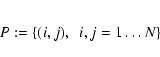
The set of indexes
.
The set of indexes
Astronomical image data contain objects on a variety of
brightness scales. Frequently stars and galaxies show up
relatively bright; arcs however are small elongated objects of
only marginally
higher intensity than the surrounding
background. In order to detect such arcs
it is necessary to correct for the dominance of extremely
bright objects. This is done by histogram modification.
Here, we use a nonlinear transformation
The interval [a,b] specifies the level of intensities where arcs are to be detected. The lower bound a is considered the intensity value of the background. By analyzing several different astronomical data sets we have learned that a and b have to be chosen relatively close to each other for optimal visualization of arcs (cf. Fig. 1).
![\begin{figure}
\par\includegraphics[width=8.8cm]{h4662f1.eps}
\end{figure}](/articles/aa/full/2004/10/aah4662/img25.gif) |
Figure 1: Distribution of pixel values of an astronomical test image. A typical parameter setting for a and b (low and high cut) is marked in gray. A good choice for parameter a is the maximum of the distribution and can be easily computed, whereas a general optimum for parameter b can not be prescribed. In the considered example a good choice is: a=0 and b=1. |
| Open with DEXTER | |
In the interval [a,b] we have to distinguish between noise and real sources such as stars,
galaxies and arcs.
To ease this separation process we apply nonlinear intensity transformations
such as
![]() ,
or alternatively s(x)=x.
,
or alternatively s(x)=x.
Some astronomical data set may contain arcs in different intensity ranges. In this case choosing the value for the parameter b of about the intensity of the brightest arcs is appropriate.
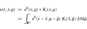
By interpolation the scaled image I0(i,j) can by interpreted as a function
in
![]() and is now denoted by
and is now denoted by
![]() .
.
By applying Gaussian convolution with a kernel
![]() depending on t one
gets a smoothed image
depending on t one
gets a smoothed image
In the following
![]() denotes the first derivative of u with respect to t,
denotes the first derivative of u with respect to t,
![]() and
and
![]() the second derivatives with respect to x and y and
the second derivatives with respect to x and y and
![]() the Laplacian.
the Laplacian.
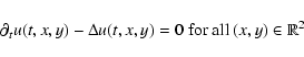
It is well known that u(t,x,y) solves the diffusion (resp. heat) equation
Equation (2) can be restricted to a rectangular domain
![]() ,
the domain of interest,
typically the set of pixels where intensity information has been recorded.
,
the domain of interest,
typically the set of pixels where intensity information has been recorded.
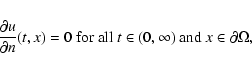
In order to achieve existence and uniqueness of the solution
![]() it is necessary to prescribe boundary conditions such as
it is necessary to prescribe boundary conditions such as
Applying the diffusion process up to a fixed time T>0 smooths the given data u0and spurious noise is filtered. The parameter T defines the strength of the filtering process. Thus in the following we refer to T as the filter parameter.
The disadvantage of Gaussian convolution is that edges in the filtered image u(T,x) are blurred and the allocation and detection of object borders is difficult. To settle this problem several advanced diffusion models have been proposed in the literature (Catte et al. 1992; Weickert 1998).
In the next section we define the general model of a diffusion process and in Sect. 2.2.3 we describe the specific model used in our algorithm.
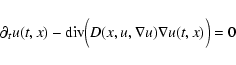
Anisotropic diffusion filtering consists in solving the time
dependent differential equation
Here
![]() is the
is the
![]() diffusion matrix depending on x and u,
diffusion matrix depending on x and u,
We prescribe the same initial and similar boundary conditions as mentioned above.
Setting
![]() results in the heat Eq. (2).
results in the heat Eq. (2).
Two classes of anisotropic diffusion models are considered in the
literature: if
![]() is independent of u and
is independent of u and ![]() then Eq. (3) is called linear anisotropic diffusion filtering,
otherwise it is called nonlinear filtering.
then Eq. (3) is called linear anisotropic diffusion filtering,
otherwise it is called nonlinear filtering.
For a survey on the topic of diffusion filtering we refer to Weickert (1998).
In anisotropic models the diffusion matrix D is constructed to reflect the estimated edge structure. That is to prefer smoothing in directions along edges, or in other words edges are preserved or even enhanced and simultaneously spurious noise is filtered.
Consequently this kind of filtering eases a subsequent edge-based object detection.
In the following D will only depend on the gradient ![]() ,
which reflects
the edge structure of the image.
,
which reflects
the edge structure of the image.
To accomplish the diffusion matrix
![]() we note that
we note that
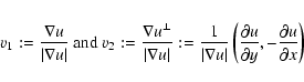
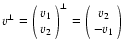 we denote the vector perpendicular to v.)
By selecting
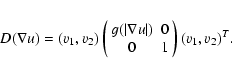
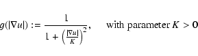
Figure 3 highlights the diffusion directions:
arrows indicate the main directions of diffusion (v1,v2) and their
thickness relates to the diffusion coefficient determining the
strength of diffusion. Parallel to the edge the diffusion
coefficient is constantly 1 (strong diffusion), where as the
diffusion coefficient
![]() in normal direction
decreases rapidly (cf. Fig. 2)
as
in normal direction
decreases rapidly (cf. Fig. 2)
as
![]() increases (weak diffusion on edges).
increases (weak diffusion on edges).
The dependence of
![]() on
on
![]() is
controlled by parameter K (cf. Fig. 2).
We therefore refer to K as the edge sensitivity parameter.
is
controlled by parameter K (cf. Fig. 2).
We therefore refer to K as the edge sensitivity parameter.
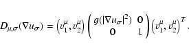
We use the following common variation of the diffusion matrix D:
To limit the effect of noise the diffusion tensor
is chosen to be dependent on the pre-smoothed image
![]() obtained by Gaussian convolution with pre-filter parameter
obtained by Gaussian convolution with pre-filter parameter ![]() .
In the following to determine the diffusion matrix
we exploit the gradient of the pre-filtered image
.
In the following to determine the diffusion matrix
we exploit the gradient of the pre-filtered image
![]() instead of u(T,.).
instead of u(T,.).
Let
![]() be the eigenvalues of the filtered
structure tensor
be the eigenvalues of the filtered
structure tensor
![\begin{eqnarray*}J_\mu(x):=\left(K_\mu *
\left[\left(\nabla u_\sigma\right)
\left(\nabla u_\sigma\right)^T\right]\right)(x).
\end{eqnarray*}](/articles/aa/full/2004/10/aah4662/img59.gif)
Note that in the case ![]() the eigenvectors of J0 are
the eigenvectors of J0 are
![]() and
and
![]() .
If
.
If ![]() and
and ![]() are small, the effect of Gaussian filtering
is negligible, and consequently
are small, the effect of Gaussian filtering
is negligible, and consequently
![]() and v1,v2 refer to similar edge structures.
and v1,v2 refer to similar edge structures.
The purpose of filtering of the structure tensor is to average information about edges in the image.
Taking into account the approximation we are led to the following
diffusion matrix
![\begin{figure}
\par\includegraphics[width=7.3cm,clip]{h4662f2.eps}
\end{figure}](/articles/aa/full/2004/10/aah4662/img69.gif) |
Figure 2: Graph plot of function g(x) used for weakening the diffusion orthogonal to edges to archive edge enhancing. For parameter K values K=0.1 resp. K=0.001 are used. |
| Open with DEXTER | |
In order to solve the differential Eq. (3) it is discretized using a finite element method in space and an implicit Euler method in time. (Within the finite element method the width of the quadratic elements is set to 1.) For each time step the resulting system of linear equations is solved by a conjugate gradient method. For a survey on solving parabolic differential equations with finite element methods we refer to Thomee (1984). The conjugate gradient method is discussed in Hanke-Bourgeois (1995,2002).
Anisotropic diffusion filtering requires to select
parameters
![]() and
and ![]() .
.
| |
Figure 3: Diffusion (smoothing) near edges: the thickness of the arrows indicate the strength of diffusion. Parallel to the edge a strong diffusion occurs whereas in orthogonal direction a weak diffusion leads to an enhancing of the edge. Due to the averaging of the structure tensor these directions are also determine the diffusion in a surrounding area of the edge and in particular at the vertices yielding a diffusion mainly parallel to the direction of elongation. |
| Open with DEXTER | |
In this section we discuss a partitioning algorithm to
separate different image data, i.e. disjoint subsets of connected
objects and background (partitions).
The algorithm uses only the anisotropic diffusion filtered data
![]() and not the initial data u0.
and not the initial data u0.
In order to save computational effort we restrict our attention to segment objects of interest, i.e. isolated objects exceeding a certain brightness.
We search for local intensity maxima exceeding a certain intensity
![]() (referred to as the intensity threshold for detection).
(referred to as the intensity threshold for detection).
Each maximum serves as seed for the partitioning algorithm: starting from the seed pixel the region to which this pixel belongs has to be determined.
To outline this concept we use the following notation.
For a given pixel
![]() we denote by N(p)the set of the eight neighboring pixels.
we denote by N(p)the set of the eight neighboring pixels.
The neighborhood of a set
![]() is the set
is the set
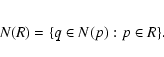
The partitioning algorithm consists of two loops.
A pixel p ![]() Pj-1 is selected where the intensity of the filtered
image u(p) attains a local maximum exceeding the intensity threshold for detection:
Pj-1 is selected where the intensity of the filtered
image u(p) attains a local maximum exceeding the intensity threshold for detection:
![]() .
.
A numerical procedure for detection of
local maxima is described in Sect. 2.3.2.
If no such pixel can be found the algorithm is terminated and Pj-1 is called "background'';
Ri consists of Ri-1 and
the neighboring pixels
![]() satisfying that
satisfying that
| |
Figure 4: Segmentation of an elliptical object (the theoretical object boundary is indicated by the black ellipse, gray squares indicate pixels with high intensities / white squares indicate pixels with low intensities): Assuming that the region growing starts with the pixel numbered by zero the neighboring pixels with numbers 1 to 7 are successively added to the region until the intensities of the next pixels to be added (here: white colored ) fall below a certain threshold intensity. |
| Open with DEXTER | |
Figure 4 illustrates the process of region growing for an elliptical objects.
A detailed overview over segmentation methods is given in Rosenfeld & Kak (1993) or Soille (2003).
In the following we describe numerical procedures for calculation of local
maxima and the determination of
![]() in the object finding algorithm.
in the object finding algorithm.
Let p0 be a local maximum within an arc, which is used as an
initialization for the region growing algorithm.
The anisotropic diffusion filtering
method calculates the two eigenvalues ![]() and
and ![]() of
the structure tensor
of
the structure tensor ![]() .
Thinking of an arc as an elliptically
shaped region
.
Thinking of an arc as an elliptically
shaped region ![]() and
and ![]() approximate the axes of the
ellipse.
approximate the axes of the
ellipse. ![]() ,
,
![]() denote the principal, respectively
cross-sectional axis. Let
denote the principal, respectively
cross-sectional axis. Let
![]() be
the intensities along the cross-sectional axes.
Figure 5 shows such a typical intensity distribution
along a cross-sectional axes of an object. The points on the cross sectional
axis with maximal gradient are natural candidates for object boundaries. In the
discrete setting these points are
be
the intensities along the cross-sectional axes.
Figure 5 shows such a typical intensity distribution
along a cross-sectional axes of an object. The points on the cross sectional
axis with maximal gradient are natural candidates for object boundaries. In the
discrete setting these points are
For the detection of local maxima which exceed the intensity threshold for detection,
![]() ,
we proceed in a similar way as in the implementation of watershed algorithms (cf. Stoev 2000).
The strategy for finding a local maximum is to choose an initial pixel p and to look for a pixel q neighboring to p with higher intensity and then with
,
we proceed in a similar way as in the implementation of watershed algorithms (cf. Stoev 2000).
The strategy for finding a local maximum is to choose an initial pixel p and to look for a pixel q neighboring to p with higher intensity and then with
![]() reinitialized to proceed iteratively until a local maximum is reached.
reinitialized to proceed iteratively until a local maximum is reached.
![\begin{figure}
\par\includegraphics[width=8cm,clip]{h4662f5.eps}
\end{figure}](/articles/aa/full/2004/10/aah4662/img98.gif) |
Figure 5: Typical intensity distribution along a cross-section through an object. |
| Open with DEXTER | |
Applying this procedure we have to deal with the case, that a local maximum may not be a single pixel but a connected set of pixels with the same intensity (a plateau). In the sequel, for simplicity of presentation, we also refer to a single pixel as a plateau.
Taking this into account we use the following procedure.
We use markers (+), (-), and (0) to denote if a pixel is a local maximum, not a local maximum, or if it is not yet considered in the algorithm, respectively. Initially every pixel is marked by (0).
After finding a local maximal plateau we choose one pixel of the plateau as seed for the later object detection.
Note that the identification of local maximal plateaus can not be carried out by investigating the first and second derivatives of the intensity function.
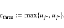
Threshold
![]() correlates to the parameters a and b. The latter should be chosen such that a is about the background intensity and b is about the intensity of the arcs to be detected. As the arc intensities are only very little higher than the noise amplitude,
correlates to the parameters a and b. The latter should be chosen such that a is about the background intensity and b is about the intensity of the arcs to be detected. As the arc intensities are only very little higher than the noise amplitude,
![]() serves as a threshold between the noise level and arcs intensity range and is of high importance for the object detection.
serves as a threshold between the noise level and arcs intensity range and is of high importance for the object detection.
Choosing
![]() guarantees detection of most objects
but many of them may result from noise amplification.
On the other hand a choice
guarantees detection of most objects
but many of them may result from noise amplification.
On the other hand a choice
![]() real arcs with intensity below
real arcs with intensity below
![]() are obviously not detected.
are obviously not detected.
Due to blurring effects on the CCD, in a neighborhood of bright stars and
galaxies, the background shows up bright, amplifying the intensity
of the noise. In these regions several local intensity maxima
above the threshold
![]() occur and regions are detected,
which clearly are artificial and belong to the background. Such
regions are singled out by a comparison of the mean intensities along
a cross section within an object and the background. To this end let
occur and regions are detected,
which clearly are artificial and belong to the background. Such
regions are singled out by a comparison of the mean intensities along
a cross section within an object and the background. To this end let
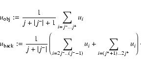
By taking into account only pixels with indices between 2j- and 2j+,
![]() averages the intensities in a small neighborhood of the object.
averages the intensities in a small neighborhood of the object.
We assume that the object is isolated, i.e. that there are
no other objects in this neighborhood and
![]() reflects the local average background intensity.
reflects the local average background intensity.
The last step of our algorithm consists in selecting arcs from the detected objects. For deriving the following features of the objects the image resulting from applying the histogram modification is used.
Let R be an object, consisting of the set of pixels
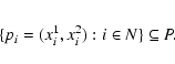

The eccentricity of R
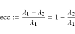
![\begin{eqnarray*}{\rm ecc} \geq c_{\rm ecc}\in[0,1] \mbox{ and }
\lambda_2 \leq c_{\rm thick}.
\end{eqnarray*}](/articles/aa/full/2004/10/aah4662/img113.gif)
The detection and selection of arcs is controlled by the
three parameters
![]() ,
,
![]() and
and
![]() :
:
In most cases the criteria described above are sufficient to detect arcs.
The selection process can be refined by incorporating a priori
information, like for instance information on the center of mass
of a gravitational lens (galaxy cluster). For a spherically symmetric
ideal
gravitational lens with center
gc=(gc1,gc2), the arcs occur
tangentially around the center.
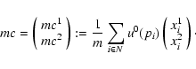
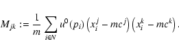
Let mc denote the center of mass
of an arc. Then the vectors p=mc-gc (position relative to center)
and ![]() (approx. direction of elongation) have to be
orthogonal, giving an additional selection criterion for arcs.
However, note that user interaction is required to incorporate
a priori information on the position of the gravitational lens.
(approx. direction of elongation) have to be
orthogonal, giving an additional selection criterion for arcs.
However, note that user interaction is required to incorporate
a priori information on the position of the gravitational lens.
The algorithm might be also used for detection of strings, if additional post-processing steps are applied using alternative selection criteria which take into account alignment information (instead of shape information as above).
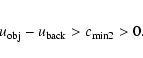
The quality of the results provided by our algorithm depends mostly on noise variance present in the data.
Arcs may not be detected (false negative detection) by the algorithm if their intensity is within the scale of the noise. As we have seen in
Sect. 2.1 the intensity range of the arcs is in general close to the background intensity.
The choice of parameter
![]() determines whether a weak structure is interpreted as background noise (ignored) or is segmented (feasible local maxima).
Corresponding the choice of a high value for
determines whether a weak structure is interpreted as background noise (ignored) or is segmented (feasible local maxima).
Corresponding the choice of a high value for
![]() increases the risk of a
false negative detection.
increases the risk of a
false negative detection.
Another case leading to a false negative detection is the joining of close-by objects.
A false positive detection may occur if the noise level exceeds the intensity
![]() .
In such case the edge enhancing anisotropic diffusion may recover structures present in the noise, which may be segmented as elongated objects afterwards.
Thus the choice of a low value for
.
In such case the edge enhancing anisotropic diffusion may recover structures present in the noise, which may be segmented as elongated objects afterwards.
Thus the choice of a low value for
![]() increases the risk of a
false positive detection.
increases the risk of a
false positive detection.
In the neighborhood of bright sources the background intensity increases and
the noise may lead to several local maxima above
![]() .
As a result the risk of a false positive detection increases in these areas.
To reduce these kinds of false positive detections we utilize the parameter
.
As a result the risk of a false positive detection increases in these areas.
To reduce these kinds of false positive detections we utilize the parameter
![]() prescribing the minimal intensity difference of a detection in comparison with its surrounding. Again the quality of detection depends on the adaption of
prescribing the minimal intensity difference of a detection in comparison with its surrounding. Again the quality of detection depends on the adaption of
![]() to the noise variance.
to the noise variance.
To highlight the properties of our algorithm we applied the algorithm
to three astronomical test images.
The first data set is an image of size 2285 ![]() 2388 pixels with intensity range
[-8.49,700.49], the second and third are of size 2048
2388 pixels with intensity range
[-8.49,700.49], the second and third are of size 2048 ![]() 2048 pixels with intensity ranges
[0,19559.8] and
[0,9314.26], respectively.
We plotted in Fig. 1 the histogram of the first data set,
the histograms of the second and third test image look similar.
2048 pixels with intensity ranges
[0,19559.8] and
[0,9314.26], respectively.
We plotted in Fig. 1 the histogram of the first data set,
the histograms of the second and third test image look similar.
Figures 6-8
show galaxy clusters with gravitationally lensed arcs, which have been
treated with histogram transformation; we have used
![]() and
(a,b)=(0,1), (149,200) and (141,170), respectively.
The histogram modification is already useful to visualize arcs.
and
(a,b)=(0,1), (149,200) and (141,170), respectively.
The histogram modification is already useful to visualize arcs.
![\begin{figure}
\par\includegraphics[width=8.15cm,clip]{h4662f6.eps}
\end{figure}](/articles/aa/full/2004/10/aah4662/img119.gif) |
Figure 6:
Detail of a VLT observation of the galaxy cluster RX J1347-1145 (from Miralles et al., in prep.). The image has a size of 2285 |
| Open with DEXTER | |
![\begin{figure}
\par\includegraphics[width=8.15cm,clip]{h4662f7.eps}
\end{figure}](/articles/aa/full/2004/10/aah4662/img120.gif) |
Figure 7:
Detail of an HST observation of the galaxy cluster A1689. The
image has a size of 2048 |
| Open with DEXTER | |
![\begin{figure}
\par\includegraphics[width=8.15cm,clip]{h4662f8.eps}
\end{figure}](/articles/aa/full/2004/10/aah4662/img121.gif) |
Figure 8:
Detail of an HST observation of the galaxy cluster A1689. The
image has a size of 2048 |
| Open with DEXTER | |
Figure 9 shows the computation
time![]() for
anisotropic diffusion filtering, object finding (including the search for local maxima, segmentation and selection) and the total computational time
in dependence of the size of the image data (number of pixels)
in typical astronomical data sets.
for
anisotropic diffusion filtering, object finding (including the search for local maxima, segmentation and selection) and the total computational time
in dependence of the size of the image data (number of pixels)
in typical astronomical data sets.
![\begin{figure}
\par\includegraphics[width=7.5cm,clip]{h4662f9.eps}
\end{figure}](/articles/aa/full/2004/10/aah4662/img122.gif) |
Figure 9: Computation time versus image size for the different steps of the algorithm. |
| Open with DEXTER | |
Numerically, the pre-filtering step is most expensive as a large system of linear equations has to be solved. The number of iterations performed by the conjugate gradient solver increases slowly with growing data size. Thus the computational effort is approximately linearly correlated to the number of pixels (cf. Fig. 9).
During the detection of local maxima each pixel is invoked a fix number of times:
Overall the total computation effort grows linearly with the image size (cf. Fig. 9).
Figure 10 shows the result of the anisotropic diffusion
filtering for the first test data set.
![\begin{figure}
\par\includegraphics[width=8.15cm,clip]{h4662f10.eps}
\end{figure}](/articles/aa/full/2004/10/aah4662/img123.gif) |
Figure 10:
Image of the cluster RX J1347-1145 with
anisotropic diffusion filtering applied. Compared to the unsmoothed
image in Fig. 6 the noise is considerably reduced.
Parameter setting for the filtering: filter parameter T=15, edge sensitivity K=0.0001, pre-filter parameter |
| Open with DEXTER | |
![\begin{figure}
\par\includegraphics[width=8.15cm,clip]{h4662f11.eps}
\end{figure}](/articles/aa/full/2004/10/aah4662/img124.gif) |
Figure 11:
Zoom of Fig. 6. Top: histogram
modified data, middle: Gaussian filtered image (Kernel |
| Open with DEXTER | |
The filter parameters were chosen to remove noise up to nearly the same
signal-to-noise ratio![]() , which is about 6.1% in the Gaussian filtered image
and about 6.3% in the image filtered with anisotropic diffusion.
, which is about 6.1% in the Gaussian filtered image
and about 6.3% in the image filtered with anisotropic diffusion.
In comparison to Gaussian convolution, anisotropic filtering is able to preserve accurately the edges of the objects both of high and of weak intensities. Anisotropic diffusion therefore is ideal as preprocessing for object finding based on edge detection.
In the first test image (Fig. 6) after applying the histogram modification about four arcs can be recognized at first glance. These arcs are grouped around a center of the cluster of galaxies, which appears in the middle of the image.
In Fig. 12 shows selected objects with
thickness
![]() and eccentricity
and eccentricity
![]() .
The eccentricity is color coded:
green, yellow, and red corresponds to an eccentricity in the ranges
[0.7, 0.8], [0.8,0.9] and [0.9,1]. The higher the eccentricity and the smaller the thickness are,
the higher is the probability that the detected object is an arc.
Incorporating a priori information on the center of the
gravitational lens, unreasonable arcs candidates can be filtered
out further (Fig. 13).
Table 1 lists the coordinates of the detected objects with
an eccentricity greater than or equal to 0.84 (referring to Fig. 12).
Besides the arcs already mentioned the algorithm detects a significant amount of arc candidates
which are not obviously recognizable to the naked eye.
.
The eccentricity is color coded:
green, yellow, and red corresponds to an eccentricity in the ranges
[0.7, 0.8], [0.8,0.9] and [0.9,1]. The higher the eccentricity and the smaller the thickness are,
the higher is the probability that the detected object is an arc.
Incorporating a priori information on the center of the
gravitational lens, unreasonable arcs candidates can be filtered
out further (Fig. 13).
Table 1 lists the coordinates of the detected objects with
an eccentricity greater than or equal to 0.84 (referring to Fig. 12).
Besides the arcs already mentioned the algorithm detects a significant amount of arc candidates
which are not obviously recognizable to the naked eye.
Figures 15 and 16 show the results of our algorithm applied to the second and third test image.
![\begin{figure}
\par\includegraphics[width=8cm,clip]{h4662f12.eps}
\end{figure}](/articles/aa/full/2004/10/aah4662/img128.gif) |
Figure 12:
Result of segmentation and
selection applied to the first test image - cluster RX J1347-1145. Only the objects which are detected as being arcs with high probability are shown. Settings:
intensity threshold for detection
|
| Open with DEXTER | |
Table 1: List of objects detected in the first data set (cf. Figs. 6 and 12) with eccentricity larger than 0.84, i.e. good arc candidates. Objects with an eccentricity larger than 0.9, i.e. objects 1 to 6 are very good candidates.
Table 2: Parameter settings used for the three test data sets.
In this section we compare our algorithm with the software package "SExtractor'' by E. Bertin (Bertin 1994; Bertin & Arnouts 1996). SExtractor is a general purpose astronomical software for the extraction of sources such as stars and galaxies, while our software is particularly designed to extract gravitationally lensed arcs. Although the main areas of applications are rather different, several levels of implementation are similar, although quite different in details: SExtractor uses background estimation which in our program is performed by histogram modification. For Detection, SExtractor used Gaussian convolution filtering; this step relates to the object finding process. Deblending and filtering of deblending are related to our merging strategy described at the second last paragraph of the last section.
To compare both algorithms we single out five specific arcs in the first test image. Figure 14 shows these objects as they are detected by the proposed algorithm (upper row) and as they are segmented by SExtractor (lower row).
Concerning the SExtractor's results a possible adaption of the SExtractor's algorithm for detection of arcs would be to perform a selection process afterwards as described in Sect. 2.4.2. However we did not apply such a selection process to the SExtractor's output. Beside the arcs under investigation several other objects with only small elongations show up when applying SExtractor. To distinguish close-by objects we use two different colors.
![\begin{figure}
\par\includegraphics[width=8cm,clip]{h4662f13.eps}
\end{figure}](/articles/aa/full/2004/10/aah4662/img129.gif) |
Figure 13: Result of segmentation and selection by taking into account a priori information on the center of the gravitational lens. The colors encode the objects eccentricity: [0.7,0.8] - green, [0.8,0.9] - yellow, [0.9,1.0] - red, i.e. the red objects are most likely arcs. The assumed center of the cluster is marked with a red cross. |
| Open with DEXTER | |
| |
Figure 14: To illustrate the features of the new algorithm we compare some specific objects detected by both algorithms, the proposed algorithm (first row) and the segmentation by SExtractor (second row). The images of each column show the same part of the image. The pixels detected by the according algorithm as belonging to the arc are plotted in red. In order to distinguish between close-by objects we use green color in addition. In Cols. 1 and 4 SExtractor has connected pixels to the arc which do actually come from various other sources. Therefore the arc may not satisfy the required elongation and hence may not be selected. Column 5 shows that the new algorithm has detected many more pixels of the faint structure than SExtractor. |
| Open with DEXTER | |
![\begin{figure}
\par\includegraphics[width=8cm,clip]{h4662f15.eps}
\end{figure}](/articles/aa/full/2004/10/aah4662/img131.gif) |
Figure 15:
Result of segmentation and selection applied to the second test image.
Parameter settings: Diffusion: filter parameter T=30, edge sensitivity K=0.0001, pre-filter parameter |
| Open with DEXTER | |
![\begin{figure}
\par\includegraphics[width=8cm,clip]{h4662f16.eps}
\end{figure}](/articles/aa/full/2004/10/aah4662/img132.gif) |
Figure 16:
Result of segmentation and selection applied to the third test image.
Parameter settings: Diffusion: filter parameter T=20, edge sensitivity K=0.0001,pre-filter parameter |
| Open with DEXTER | |
The first remarkable difference is that SExtractor in order to measure the objects total magnitudes uses a far lower segmentation threshold and thus it segments larger parts of bright objects than our algorithm as can be realized in columns one to three in Fig. 14. The evaluation of the objects elongation then depends on the segmented shape.
The results of our algorithm show a more regular border due to the edge parallel diffusion and the edge enhancement. Using SExtractor one may choose a higher threshold for detection (DETECT_THRES) and yield a better shape of the segmented objects. However, since this is a global threshold SExtractor tends to loose fainter objects. Our algorithm overcomes this problem by using a local adaptive threshold.
The forth arc in Fig. 14 segmented by SExtractor is an example for a failure of the deblending procedure. The arc is not separated from the nearby galaxy and since the composition of both sources is not much elongated it would be refused by the selection process. On the other hand tuning the parameter for deblending, which is supplied by SExtractor for this specific arc allows a separate detection of both sources but leads to an undesired splitting of other objects.
In the fifth arc our algorithm reveals a far larger part of the weak structure than SExtractor due to the use of anisotropic diffusion and detects its direction of elongation correctly. SExtractor does also find an elongated part of this arc but the direction of elongation of this part differs from the exact direction. Thus our algorithm provides a better quality of detection.
To summarize the new algorithm for detecting arcs presented here has two main advantages.
The method of filtering, e.g. anisotropic diffusion is chosen with regard to the kind of objects to be detected. The filtering process provides a closure of gaps in between objects as well as edge enhancing.
The use of object dependent thresholds based on edge detection leads to an improved segmentation even of weak sources. A deblending procedure is not required. Moreover the new algorithm is able to detect close-by objects of different scale, for which the SExtractor's deblending procedure fails.
We proposed a new algorithm for the detection of gravitationally lensed arcs on CCD images of galaxy clusters, performing an edge-based object detection on the filtered image together with an automatic selection of arcs.
The algorithm consists of several steps:
The new algorithm is particularly well suited for the detection of arcs in astronomical images. It can be both applied to automated surveys as well as to individual clusters.
The algorithm (implemented in C) will be provided to the public. Feel free to contact Frank Lenzen (Frank.Lenzen@uibk.ac.at).
Acknowledgements
We thank Thomas Erben and Peter Schneider for kindly providing the HST image of A1689. We are grateful to Joachim Wambsganss and Thomas Erben for valuable comments to the manuscript.The work of F.L. is supported by the Tiroler Zukunftsstiftung. The work of O.S. and S.S. is partly supported by the Austrian Science Foundation, Projects Y-123INF and P15868, respectively.
![\begin{displaymath}%
\mathcal{S}(x)=\left\{
\begin{array}{cl}
0&\mbox{ if }x<a\\...
...\mbox{ if } x\in [a,b]\\
1&\mbox{ if } x>b
\end{array}\right.
\end{displaymath}](/articles/aa/full/2004/10/aah4662/img22.gif)