A&A 415, 349-376 (2004)
DOI: 10.1051/0004-6361:20034594
T. Repolust1 - J. Puls1 - A. Herrero2,3
1 - Universitäts-Sternwarte München, Scheinerstr. 1, 81679 München,
Germany
2 -
Instituto de Astrofísica de Canarias, 38200 La Laguna,
Tenerife, Spain
3 -
Departamento de Astrofísica, Universidad de La Laguna,
Avda. Astrofísico Francisco Sánchez, s/n, 38071 La Laguna, Spain
Received 20 May 2003 / Accepted 17 October 2003
Abstract
We have re-analyzed the Galactic O-star sample from Puls et al. (1996)
by means of line-blanketed NLTE model atmospheres in order to investigate
the influence of line-blocking/blanketing on the derived parameters. The
analysis has been carried out by fitting the photospheric and wind lines
from H and He. In most cases we obtained a good fit, but we have
also found certain inconsistencies which are probably related to a still
inadequate treatment of the wind structure. These inconsistencies comprise
the line cores of H
![]() and H
and H
![]() in supergiants (the synthetic profiles are
too weak when the mass-loss rate is determined by matching H
in supergiants (the synthetic profiles are
too weak when the mass-loss rate is determined by matching H
![]() )
and the
"generalized dilution effect'' (cf. Voels et al. 1989) which is still present
in He I 4471 of cooler supergiants and giants.
)
and the
"generalized dilution effect'' (cf. Voels et al. 1989) which is still present
in He I 4471 of cooler supergiants and giants.
Compared to pure H/He plane-parallel models we found a decrease in
effective temperatures which is largest at earliest spectral types
and for supergiants (with a maximum shift of roughly 8000 K).
This finding is explained by the fact that line-blanketed models of hot
stars have photospheric He ionization fractions similar to those from
unblanketed models at higher
![]() and higher
and higher ![]() .
Consequently, any
line-blanketed analysis based on the He ionization equilibrium results in
lower
.
Consequently, any
line-blanketed analysis based on the He ionization equilibrium results in
lower
![]() -values along with a reduction of either
-values along with a reduction of either ![]() or helium
abundance (if the reduction of
or helium
abundance (if the reduction of ![]() is prohibited by the Balmer line wings).
Stellar radii and mass-loss rates, on the other hand, remain more or less
unaffected by line-blanketing.
is prohibited by the Balmer line wings).
Stellar radii and mass-loss rates, on the other hand, remain more or less
unaffected by line-blanketing.
We have calculated "new'' spectroscopic masses and compared them with
previous results. Although the former mass discrepancy (Herrero et al. 1992)
becomes significantly reduced, a systematic trend for masses below 50
![]() seems to remain: The spectroscopically derived values are smaller than the
"evolutionary masses'' by roughly 10
seems to remain: The spectroscopically derived values are smaller than the
"evolutionary masses'' by roughly 10
![]() .
Additionally, a significant
fraction of our sample stars stays over-abundant in He, although the actual
values were found to be lower than previously determined.
.
Additionally, a significant
fraction of our sample stars stays over-abundant in He, although the actual
values were found to be lower than previously determined.
Also the wind-momentum luminosity relation (WLR) changes because of lower luminosities and almost unmodified wind-momentum rates. Compared to previous results, the separation of the WLR as a function of luminosity class is still present but now the WLR for giants/dwarfs is consistent with theoretical predictions.
We argue that the derived mass-loss rates of stars
with H
![]() in emission are affected by clumping in the lower wind
region. If the predictions from different and independent theoretical
simulations (Puls et al. 2003a; Vink et al. 2000; Pauldrach et al. 2003) that the WLR should be
independent of luminosity class were correct, a typical clumping factor
in emission are affected by clumping in the lower wind
region. If the predictions from different and independent theoretical
simulations (Puls et al. 2003a; Vink et al. 2000; Pauldrach et al. 2003) that the WLR should be
independent of luminosity class were correct, a typical clumping factor
![]() should be derived by "unifying'' the different WLRs.
should be derived by "unifying'' the different WLRs.
Key words: stars: atmospheres - stars: distances - stars: early-type - stars: fundamental parameters - stars: mass loss - stars: winds, outflows
The understanding of massive stars and their evolution is not only fundamental to stellar astrophysics but it also provides insights into a variety of other processes. Massive star winds (with parameters depending on evolutionary stage and environment) are crucial for the chemical and dynamical evolution of galaxies through their input of energy, momentum, and nuclear processed material into the interstellar medium (e.g., Oey 2003; Silich & Tenorio-Tagle 2001; Leitherer & Heckman 1995). In the distant Universe, massive stars dominate the integrated UV-light of very young galaxies (Steidel et al. 1996; Pettini et al. 2000); even earlier they are the suspected sources of the re-ionization of the Universe (Bromm et al. 2001).
Thus, by observing and analyzing massive stars we can (in principle) provide the numbers required to tackle these problems. Moreover, we can address a number of ensuing questions which are of great interest and might have significant consequences for our general understanding. Present efforts, for example, concentrate on the physics of rotation (with respect to both the interior structure by means of mixing processes and the exterior structure by modifying the wind morphology, e.g. Maeder & Meynet 2000 and references therein), the influence of time-dependent processes (see below) and the so-called wind-momentum luminosity relation (WLR) which might become an independent tool to derive extragalactic distances on an intermediate scale (up to the Virgo and Fornax cluster).
This knowledge is mainly derived from the analysis of stellar spectra which in turn requires adequate atmospheric models. For this purpose sophisticated model atmosphere codes have been developed in the last decade, e.g., Hubeny & Lanz (1995), Santolaya-Rey et al. (1997, ''FASTWIND''), Hillier et al. (1998), Pauldrach et al. (2001) and Gräfener et al. (2002) which incorporate detailed atomic models and improved numerical techniques. These models offer us the opportunity to derive rather realistic stellar parameters and provide insight into the chemical composition of stars. Additionally, the latter four codes allow for an investigation of important wind properties such as mass-loss rates, wind terminal velocities and velocity structures.
Considering that the actual value of the mass-loss rate
has a significant influence on massive star evolution![]() , the derived
mass-loss rates need to be known to a level of precision better than a
factor of two; otherwise, evolutionary calculations relying on these numbers
could become completely erroneous.
, the derived
mass-loss rates need to be known to a level of precision better than a
factor of two; otherwise, evolutionary calculations relying on these numbers
could become completely erroneous.
Although such a precision is feasible (at least differentially, cf. Kudritzki & Puls 2000 and references therein), the situation looks different on an absolute scale. Most important in this sense is the fact that stellar rotation (e.g., Maeder & Meynet 2000a), the intrinsic instability of the line-driving mechanism (Owocki et al. 1988; Feldmeier 1995; Owocki & Puls 1999) and their interaction (Owocki 1999) are able to produce non-spherical and inhomogeneous structures, observationally evident, e.g., from X-ray emission and line profile variability. Unless we completely understand these structures, we cannot be entirely sure about the "average'' properties of stellar winds like mass-loss rates and ionizing fluxes. At least in the case of WR-stars, the presence of clumping has severe consequences for the interpretation of observed line profiles, particularly with respect to the derived mass-loss rates, e.g., Moffat & Robert (1994), Schmutz (1997).
Not only do present mass-loss rates remain somewhat uncertain but also the basic stellar parameters of O-stars are subjected to a number of uncertainties. Using plane-parallel NLTE-models, Herrero et al. (1992) have presented discrepancies in masses and helium abundances of O-stars, derived from either evolutionary tracks or spectroscopy. It was suggested that these discrepancies could be reduced by accounting for rotational mixing in the evolutionary calculations (which partly turned out to be true, Meynet & Maeder 2000) and/or by including the effects of mass-loss and sphericity into the atmospheric models.
The latter deficiency was corrected when so-called unified model atmospheres became available (Gabler et al. 1989). On the basis of these models, Puls et al. (1996) introduced an approximate method to obtain mass-loss estimates for a large sample of Galactic and Magellanic Cloud O-stars. As a "by-product'', this analysis provided the basis for the wind-momentum luminosity relationship of hot stars (Kudritzki et al. 1995).
There is, however, one additionally important effect that could not be treated at that time: the influence of line-blocking/blanketing which should significantly affect the analysis, mainly with respect to the temperature scale as a function of spectral type. With the present generation of atmospheric model codes this task has now become feasible.
Recently Martins et al. (2002) have presented such a new temperature scale for massive O dwarfs that is actually considerably lower than the one found by Vacca et al. (1996) (based on plane-parallel, pure H/He model atmospheres) as a result of strong metal line blanketing. Crowther et al. (2002) have presented an analysis of four supergiants in the LMC and SMC with similar but stronger trends, and Herrero et al. (2002) have analyzed seven Cyg OB2 stars by means of the latest, line-blanketed version of FASTWIND.
In view of the important role of hot stars and their winds, a re-analysis of the O-star sample by Puls et al. (1996) is urgently required, particularly because this sample still comprises the basic data set for O-star mass-loss rates and corresponding WLRs.
In the present paper we will first concentrate on the Galactic sub-sample and on a detailed spectral analysis of the corresponding stars and then comment on peculiarities, problems and uncertainties, mainly on the basis of a differential comparison with previous results from unblanketed models. Preliminary results of our investigation have already been published in Puls et al. (2003a).
The remainder of this paper is organized as follows. In Sect. 2 we briefly outline the characteristics of the code used, followed by a description of our Galactic sample in Sect. 3. Section 4 comprises general remarks on our procedure and summarizes the basic results of our analysis in Table 1. In Sect. 5, we comment in detail on our individual objects and in Sect. 6 we present an elaborated error analysis. In Sect. 7 we discuss the implications of our investigation: First, we consider the relation between effective temperature vs. spectral type and gravity vs. effective temperature in view of the new results. We then explain the differences in the results from blanketed and unblanketed models in fair detail and comment on the status quo of mass and helium discrepancies outlined above and present an updated view of the WLR for Galactic O-type stars. Finally, Sect. 8 comprises further conclusions and a summary of this work.
The code comprises the concept of "unified model atmospheres'' (i.e., the smooth transition from a pseudo-hydrostatic photosphere to a wind) along with an appropriate treatment of line-broadening which is a prerequisite for the analysis of O-stars of different luminosity classes covering a variety of wind densities.
The approximations underlying the treatment of metal line
blocking/blanketing will be described in detail by Puls et al. (2003b, in prep.). In
summary, the calculation of the required NLTE metal opacities (bound-bound,
bound-free, and free-free) follows the principal philosophy presented by
Abbott & Lucy (1985), Schmutz (1991), Schaerer & Schmutz (1994) and Puls et al. (2000) and
important details have now been improved upon. Particularly, the equations
of approximate ionization equilibrium have been re-formulated to account for
the actual radiation field as a function of depth at all ionization
edges, and a consistent iteration scheme regarding the coupling of the rate
equations and the radiation field has been established to avoid the
well-known convergence problems of a pure Lambda Iteration. For the
calculation of the effects of line-blocking, we used suitable means for the
line opacities, averaged over a frequency interval of the order of
![]() ,
while flux conservation (line-blanketing!) is obtained by incorporating the
concept of NLTE-Hopf parameters (cf. Santolaya-Rey et al. 1997) in a
consistent way.
,
while flux conservation (line-blanketing!) is obtained by incorporating the
concept of NLTE-Hopf parameters (cf. Santolaya-Rey et al. 1997) in a
consistent way.
The code has carefully been tested by comparison with
results from alternative, fully blanketed codes presently available. On
the one hand, we have compared our blanketed fluxes with those from the
model-grid![]() provided by Pauldrach et al. (2001, WMbasic), and
found very good agreement in almost all cases. Some of the complementary
tests, on the other hand, have already been discussed by Herrero et al. (2002, see also
Urbaneja et al. 2003). As an example for stars with negligible winds, the
analysis of 10 Lac (O9 V) resulted in an excellent fit at temperatures lower
than those obtained from unblanketed models, and the derived parameters
completely agree with those obtained by Hubeny et al. (1998) using TLUSTY.
With respect to CMFGEN, direct as well as indirect tests have
been performed. As an example of direct tests, Herrero et al. (2002) have compared the
emergent fluxes resulting from FASTWIND and CMFGEN for a model
of Cyg OB2
provided by Pauldrach et al. (2001, WMbasic), and
found very good agreement in almost all cases. Some of the complementary
tests, on the other hand, have already been discussed by Herrero et al. (2002, see also
Urbaneja et al. 2003). As an example for stars with negligible winds, the
analysis of 10 Lac (O9 V) resulted in an excellent fit at temperatures lower
than those obtained from unblanketed models, and the derived parameters
completely agree with those obtained by Hubeny et al. (1998) using TLUSTY.
With respect to CMFGEN, direct as well as indirect tests have
been performed. As an example of direct tests, Herrero et al. (2002) have compared the
emergent fluxes resulting from FASTWIND and CMFGEN for a model
of Cyg OB2 ![]() 7 (O3 If*), and again found remarkable agreement between
both codes for this hot supergiant with strong wind. Unpublished indirect
tests (Najarro, priv. commun.) concern an alternative combined UV/optical
analysis, performed for a part of the Cyg OB2 objects from Herrero et al. (2002) by
means of CMFGEN. For two objects (Cyg OB2
7 (O3 If*), and again found remarkable agreement between
both codes for this hot supergiant with strong wind. Unpublished indirect
tests (Najarro, priv. commun.) concern an alternative combined UV/optical
analysis, performed for a part of the Cyg OB2 objects from Herrero et al. (2002) by
means of CMFGEN. For two objects (Cyg OB2 ![]() 4 (O7 III ((f))) and
4 (O7 III ((f))) and
![]() 10 (O9.5 I) excellent agreement in all derived parameters was obtained,
whereas for two other objects (Cyg OB2
10 (O9.5 I) excellent agreement in all derived parameters was obtained,
whereas for two other objects (Cyg OB2 ![]() 11 (O5 If*) and
11 (O5 If*) and ![]() 8A (O5.5 I(f)) somewhat cooler temperatures (and accordingly also lower mass-loss rates)
have been derived. The origin of this inconsistency (the only one arising so
far) is still unclear and will be analyzed in a forthcoming investigation.
Note, however, that an independent CMFGEN analysis of
8A (O5.5 I(f)) somewhat cooler temperatures (and accordingly also lower mass-loss rates)
have been derived. The origin of this inconsistency (the only one arising so
far) is still unclear and will be analyzed in a forthcoming investigation.
Note, however, that an independent CMFGEN analysis of ![]() Pup (O4 I(f)) performed by Crowther et al. (2002) resulted in very similar
parameters as found in the present work (cf. Sect. 7.1).
Pup (O4 I(f)) performed by Crowther et al. (2002) resulted in very similar
parameters as found in the present work (cf. Sect. 7.1).
For our re-analysis we have used the spectra described by Herrero et al. (1992) and
Puls et al. (1996). The H
![]() observations of the core sample of Galactic O-stars
were taken from Herrero et al. (1992) and Herrero (1993) and were carried out with the 2.5 m
Isaac Newton telescope at the Observatory of El Roque de los Muchachos in La
Palma in July and October 1989 and in August 1992. The blue observations
needed to derive photospheric parameters were obtained during the same runs
with an additional one in September 1991.
Note however that the blue and red spectra were not taken simultaneously.
For a specific observational run, all red spectra were obtained
during one night, whereas the blue spectra were collected
during the remaining nights.
observations of the core sample of Galactic O-stars
were taken from Herrero et al. (1992) and Herrero (1993) and were carried out with the 2.5 m
Isaac Newton telescope at the Observatory of El Roque de los Muchachos in La
Palma in July and October 1989 and in August 1992. The blue observations
needed to derive photospheric parameters were obtained during the same runs
with an additional one in September 1991.
Note however that the blue and red spectra were not taken simultaneously.
For a specific observational run, all red spectra were obtained
during one night, whereas the blue spectra were collected
during the remaining nights.
The Intermediate Dispersion
Spectrograph (IDS) was used with the 1800 V grating along with the 235 mm
camera yielding a spectral resolution of 0.8 Å FWHM along with a measured S/N ratio of ![]() 300 and a spectral resolution of 0.6 Å FWHM along
with a S/N ratio ranging from 150 to 200 for the red and the blue
observations, respectively. The reduction of the data was made following
standard procedures (using various packages such as IRAF, FIGARO
(Shortridge 1987), Midas etc.) comprising bias subtraction, flat field
division, spectrum extraction, wavelength calibration and continuum
rectification.
300 and a spectral resolution of 0.6 Å FWHM along
with a S/N ratio ranging from 150 to 200 for the red and the blue
observations, respectively. The reduction of the data was made following
standard procedures (using various packages such as IRAF, FIGARO
(Shortridge 1987), Midas etc.) comprising bias subtraction, flat field
division, spectrum extraction, wavelength calibration and continuum
rectification.
The above data is supplemented by additional O3 stars located in the Carina
nebula and some further well-observed stars such as ![]() Pup and
Pup and ![]() Cam. The data for the Carina stars (HD 93129A, HD 93128, HD 93250, and
HD 303308) were obtained in December 1992 using the ESO New Technology
Telescope (NTT) and the EMMI spectrograph covering the wavelength ranges
3920-4380, 4300-4750 and 6300-6800 Å at a resolution of 0.9, 0.95 and
1.1 Å, respectively. The measured S/N ratio was found to be of the order of
Cam. The data for the Carina stars (HD 93129A, HD 93128, HD 93250, and
HD 303308) were obtained in December 1992 using the ESO New Technology
Telescope (NTT) and the EMMI spectrograph covering the wavelength ranges
3920-4380, 4300-4750 and 6300-6800 Å at a resolution of 0.9, 0.95 and
1.1 Å, respectively. The measured S/N ratio was found to be of the order of
![]() 200.
200.
Furthermore, additional red spectrograms of HD 207198, and HD 209975 were obtained with a similar instrumental setup as described by Herrero et al. (1992) and Herrero (1993).
The blue spectra of ![]() Cam were taken from Lennon et al. (1992), and the red
ones from Lennon et al. (1993).
Cam were taken from Lennon et al. (1992), and the red
ones from Lennon et al. (1993).
The data for ![]() Pup (blue and red), finally, was taken from
Bohannan et al. (1990), where further information of the observational material and
data reduction procedures may be found.
Pup (blue and red), finally, was taken from
Bohannan et al. (1990), where further information of the observational material and
data reduction procedures may be found.
For all spectra we used the rectifications provided by the corresponding observers. Note, however, that particularly the region around the "new'' He I/He II lines in the red band (see below) suffers from some problems in rectification, since this region has not been considered in detail before. Nevertheless, we have refrained from any "re-rectification'' and have commented on the problem when present.
In total the sample consists of 24 Galactic O-stars as listed in Table 1 covering luminosity class I, III, and V objects.
Table 1:
Galactic O-star sample: Stellar and wind parameters adopted (![]() )
and derived using FASTWIND.
)
and derived using FASTWIND.
![]() in kK,
in kK, ![]() in
in
![]() ,
,
![]() sini and
sini and
![]() in km s-1,
in km s-1, ![]() in
in
![]() ,
L in
,
L in
![]() ,
,
![]() in 10-6
in 10-6
![]() /yr
(terminal velocities
/yr
(terminal velocities
![]() from Paper I). HD 93129A and HD 303308 have
recently been detected as binary systems but they are treated here as single
stars (see text). Bold face numbers denote
from Paper I). HD 93129A and HD 303308 have
recently been detected as binary systems but they are treated here as single
stars (see text). Bold face numbers denote ![]() -values which could be
derived with high precision from emission profiles. Stars with absorption
profiles were fitted with an assumed value of
-values which could be
derived with high precision from emission profiles. Stars with absorption
profiles were fitted with an assumed value of
![]() .
.
![]() is the stellar radius resulting from our new models which was
calculated by means of the "old''
is the stellar radius resulting from our new models which was
calculated by means of the "old'' ![]() values from Paper I (not tabulated
here).
values from Paper I (not tabulated
here).
Before presenting the detailed results of our analysis, we would like to remark on certain aspects concerning our procedure.
Nevertheless, we still have to consider the runaway or field stars in
the sample. Four of them have measured H IPPARCOS parallaxes
(ESA 1997) with not
too large errors: HD 66811 (![]() Pup), HD 210839 (
Pup), HD 210839 (![]() Cep),
HD 24912 (
Cep),
HD 24912 (![]() Per) and HD 149757 (
Per) and HD 149757 (![]() Oph). In these cases, however,
we have to consider the uncertainty in the derived absolute magnitudes
introduced by the Lutz-Kelker effect (Lutz & Kelker 1973). Only
Oph). In these cases, however,
we have to consider the uncertainty in the derived absolute magnitudes
introduced by the Lutz-Kelker effect (Lutz & Kelker 1973). Only ![]() Oph has
a relative error that allows a standard correction of the Lutz-Kelker effect
and we adopt the value derived from the measured parallax and the correction
provided by Koen (1992). We have reduced the 90
Oph has
a relative error that allows a standard correction of the Lutz-Kelker effect
and we adopt the value derived from the measured parallax and the correction
provided by Koen (1992). We have reduced the 90![]() confidence limits
provided by Koen to the usual standard deviation for our errors.
confidence limits
provided by Koen to the usual standard deviation for our errors.
The relative error in the parallax of ![]() Pup is slightly beyond the
limit for which the standard Lutz-Kelker correction can be applied. We have
estimated the correction using Fig. 2 in Oudmajier et al. (1998) and have found that
the resulting value agrees well with existing calibrations of absolute
magnitude versus spectral classification (e.g., Massey 1998 or
Walborn 1972). Therefore, we have adopted this resulting value and
corresponding uncertainty (i.e.,
Pup is slightly beyond the
limit for which the standard Lutz-Kelker correction can be applied. We have
estimated the correction using Fig. 2 in Oudmajier et al. (1998) and have found that
the resulting value agrees well with existing calibrations of absolute
magnitude versus spectral classification (e.g., Massey 1998 or
Walborn 1972). Therefore, we have adopted this resulting value and
corresponding uncertainty (i.e., ![]() 0.43 mag which is larger than the
uncertainty adopted for most of the stars).
0.43 mag which is larger than the
uncertainty adopted for most of the stars).
We have performed the same exercise for ![]() Cep, but the resulting
value did not comply with current calibrations. We preferred the absolute
magnitude from spectroscopic parallaxes given in the literature, in
particular the value provided by Garmany & Stencel (1992) since its agreement with
existing calibrations is better. Additionally, we adopted a larger
uncertainty in absolute magnitude,
Cep, but the resulting
value did not comply with current calibrations. We preferred the absolute
magnitude from spectroscopic parallaxes given in the literature, in
particular the value provided by Garmany & Stencel (1992) since its agreement with
existing calibrations is better. Additionally, we adopted a larger
uncertainty in absolute magnitude, ![]() 0.5 mag.
0.5 mag.
![]() Per has the largest relative error in the measured parallax and the
absolute magnitudes found in the literature do not match its spectral
classification (de Zeeuw et al. 1999; Humphreys 1978; Hoogerwerf et al. 2001). Therefore, we adopt a
value from the calibrations by Massey (1998) and Walborn (1972).
Per has the largest relative error in the measured parallax and the
absolute magnitudes found in the literature do not match its spectral
classification (de Zeeuw et al. 1999; Humphreys 1978; Hoogerwerf et al. 2001). Therefore, we adopt a
value from the calibrations by Massey (1998) and Walborn (1972).
For HD 30614 (![]() Cam), finally, we have used the absolute magnitude
taken from the calibration by Walborn (1972)
Cam), finally, we have used the absolute magnitude
taken from the calibration by Walborn (1972)![]() .
.
Compared to the
"old'' values from Paper I, the "new'' absolute magnitudes remain almost
unchanged (typical modifications are of the order of
![]() mag) except for the following cases:
mag) except for the following cases: ![]() Per,
Per, ![]() Cam and HD 209975
have become brighter by 0.4, 0.9 and 0.7 mag, respectively, whereas
HD 217086 has become fainter by 0.4 mag.
Cam and HD 209975
have become brighter by 0.4, 0.9 and 0.7 mag, respectively, whereas
HD 217086 has become fainter by 0.4 mag.
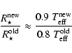
From these ![]() -values, stellar radii have been calculated
following the procedure outlined by Kudritzki (1980) and Herrero et al. (1992):
-values, stellar radii have been calculated
following the procedure outlined by Kudritzki (1980) and Herrero et al. (1992):
The input radii used as starting values for our atmospheric models
were taken from Paper I and have been calculated from the "old'' ![]() -values
provided by Herrero et al. (1992) and Paper I. Since the inclusion of line
blocking/blanketing changes the theoretical fluxes (cf.
Sect. 7.2) and since we have adopted somewhat different values
for
-values
provided by Herrero et al. (1992) and Paper I. Since the inclusion of line
blocking/blanketing changes the theoretical fluxes (cf.
Sect. 7.2) and since we have adopted somewhat different values
for ![]() (see above), the radii change accordingly which has been accounted
for in the calculation of the final models. Even for the largest
modifications of
(see above), the radii change accordingly which has been accounted
for in the calculation of the final models. Even for the largest
modifications of ![]() ,
the changes in radius remain below 25%,
except for
,
the changes in radius remain below 25%,
except for ![]() Cam, with an increase in radius by 50%,
cf. Table 1.
Cam, with an increase in radius by 50%,
cf. Table 1.
Note that in Table 1 all radius-dependent quantities such as
luminosity, mass and mass-loss rate refer to the stellar radii calculated
from the ![]() -values as described above ("
-values as described above ("![]() ''), since we regard these
values as superior to the "older'' ones. However, we additionally
provide stellar radii calculated from the "old''
''), since we regard these
values as superior to the "older'' ones. However, we additionally
provide stellar radii calculated from the "old'' ![]() -values
("
-values
("
![]() ''). Hence,
''). Hence,
![]() can easily be rescaled (e.g., Sect. 7.5), accounting for the fact that
a strictly differential comparison with earlier analyses is
one of the primary objectives of the present work.
can easily be rescaled (e.g., Sect. 7.5), accounting for the fact that
a strictly differential comparison with earlier analyses is
one of the primary objectives of the present work.
Moreover, according to Walborn et al. (2002), HD 93129A and HD 303308 (prior to knowing that the two stars were binaries; see Nelan et al. 2003, in prep.) have been revised to O2 If* and O4 V((f+)), respectively.
In former analyses mainly two He II lines, He II ![]()
![]() 4200 and 4541
(n = 4
4200 and 4541
(n = 4
![]() 11 and n = 4
11 and n = 4
![]() 9) have been used to derive the stellar
parameters, since He II 4686, on many occasions, is affected by severe wind
emission which could not be synthesized from plane-parallel models. Moreover,
He II 4686 depends strongly on the behaviour of the He II resonance line
at 303 Å, which in turn reacts sensitively to the details of line-blocking
(as all other He II resonance lines do).
9) have been used to derive the stellar
parameters, since He II 4686, on many occasions, is affected by severe wind
emission which could not be synthesized from plane-parallel models. Moreover,
He II 4686 depends strongly on the behaviour of the He II resonance line
at 303 Å, which in turn reacts sensitively to the details of line-blocking
(as all other He II resonance lines do).
Since the present code can deal with both winds and line-blocking, this line has now been included and serves as an ideal tool to indirectly check the accuracy of the calculated line-blocking in the EUV.
Moreover, as already mentioned, we have included the He lines located
blue- and redwards of H
![]() into our analysis, providing additional
constraints and information on the sensitivity to small parametric changes
and thus allowing to check the consistency of our assumptions and results.
In particular, we added the two He II lines at 6404 Å and 6527 Å bluewards of H
into our analysis, providing additional
constraints and information on the sensitivity to small parametric changes
and thus allowing to check the consistency of our assumptions and results.
In particular, we added the two He II lines at 6404 Å and 6527 Å bluewards of H
![]() with corresponding transitions n = 5
with corresponding transitions n = 5
![]() 15 and
n = 5
15 and
n = 5
![]() 14, respectively.
Redwards of H
14, respectively.
Redwards of H
![]() we included He II 6683 (n = 5
we included He II 6683 (n = 5
![]() 13) which is blended
with He I 6678. The latter line belongs to the singlet system with lower level
(
13) which is blended
with He I 6678. The latter line belongs to the singlet system with lower level
(
![]() )
and upper level (
)
and upper level (
![]() ).
).
Before beginning to comment on the individual
objects, we would like to point out some general behaviour of the
fitted lines.
On the other hand, for those supergiants with
![]()
![]() K we
either obtain a good fit quality for all Balmer lines or (in two cases) H
K we
either obtain a good fit quality for all Balmer lines or (in two cases) H
![]() and/or H
and/or H
![]() show too little wind emission in their cores.
show too little wind emission in their cores.
"Historically'', this effect expresses the strengthening of the He I absorption lines with decreasing effective temperature (see Voels et al. 1989 and references therein) and has been invoked to explain certain deviations between synthetic line profiles from plane-parallel models and observations in cool O-supergiants: in this spectral range, one usually finds that a number of synthetic He I lines are considerably weaker than the observations, whereas this effect is most prominent for He I 4471.
The conventional explanation assumes that the lower levels of
the corresponding transitions, 2![]() ,2
,2![]() ,
2
,
2![]() ,
and
2
,
and
2![]() become overpopulated (with decreasing degree of overpopulation)
because of the dilution of the radiation field in the (lower) wind.
Note that the NLTE departure
coefficients scale with the inverse of the dilution factor, since the
ionization rates are proportional to this quantity (less ionization from a
diluted radiation field), whereas the recombination rates remain unaffected.
become overpopulated (with decreasing degree of overpopulation)
because of the dilution of the radiation field in the (lower) wind.
Note that the NLTE departure
coefficients scale with the inverse of the dilution factor, since the
ionization rates are proportional to this quantity (less ionization from a
diluted radiation field), whereas the recombination rates remain unaffected.
Once more, this explanation is based on principal theoretical considerations, without any direct proof by actual simulations accounting for an extended atmosphere.
From the results of our simulations (which now include such a treatment), however, it is obvious that there still might be something missing in the above interpretation. In particular He I 4471 is still too weak in cooler supergiants, even if we account for a significant micro-turbulence (see above). Again, this finding is supported by previous investigations from Herrero et al. (2002,2000).
Another consequence of the above theoretical scenario would be the following: For each of the lower He I levels under consideration, the lines belonging to one series should become less affected by the dilution of the radiation field with decreasing oscillator strength, since the line is formed at increasingly greater depths.
This would imply, e.g., that He I 6678 with lower level 2![]() (larger oscillator strength but less
overpopulated lower level) should approximately be as strongly
affected by dilution as He I 4471 (with lower level 2
(larger oscillator strength but less
overpopulated lower level) should approximately be as strongly
affected by dilution as He I 4471 (with lower level 2![]() ).
From our results, however, we can see that also this prediction
does not hold if checked by simulations. A typical example is
).
From our results, however, we can see that also this prediction
does not hold if checked by simulations. A typical example is ![]() Cam:
Although He I 4471 is too weak, He I 6678 can perfectly be fitted.
Cam:
Although He I 4471 is too weak, He I 6678 can perfectly be fitted.
At least for all other lines investigated, the prediction seems to hold. The weakest transitions in each series, i.e., the He I 4713 triplet line and the He I 4387 singlet line, give very good line fits and the same is true for He I 4922.
Hence, the only line with prominent generalized dilution effect (we keep this denotation) is He I 4471 and cannot be reproduced by our code even if line-blocking/blanketing is included. Similarly, it is rather improbable that a too large wind emission in the line core (as found for the blue Balmer lines) is the reason for this "defect'', since this problems seems to be present only in hotter supergiants. For the cooler ones, where He I 4471 is too weak, the line cores of all other lines are equally well described.
Thus, the actual origin of the dilution effect in He I 4471 is unclear, although a tight relation to either luminosity and/or the presence of a (strong) wind seems to be obvious: dwarfs do not suffer from this effect, no matter if early or late type dwarfs, as can be seen from the almost perfect fit quality of He I 4471 in these cases (Fig. 8).
On the other hand, all O-type class I and III objects between O6 and O9.5 show too weak He I 4471, whereas stars earlier than O6 behave like class V objects, i.e., they pose no problem.
The boundary for the onset of the dilution effect, however, is
difficult to determine. Our model calculations of HD 210839 (O6 I(n) fp)
which constitutes an upper boundary for the effect in class I objects
reveal that a decrease in
![]() or
or ![]() along with corresponding
changes in
along with corresponding
changes in ![]() helps to improve the H
helps to improve the H
![]() ,
H
,
H
![]() and He I 4471 line fits,
whereas the good fit quality for the other lines is lost in this case.
The situation is similar for HD 190864 (O6.5 III(f)).
No matter which sensible parametric alterations we applied,
there were hardly any changes in He I 4471.
and He I 4471 line fits,
whereas the good fit quality for the other lines is lost in this case.
The situation is similar for HD 190864 (O6.5 III(f)).
No matter which sensible parametric alterations we applied,
there were hardly any changes in He I 4471.
From these experiments, we estimate the upper boundary for the presence of the dilution effect to lie somewhere between O6 and O6.5 for class I and III objects.
It cannot be excluded, of course, that the discussed effect is a deficiency of the present version of FASTWIND. Combined UV/optical CMFGEN analyses by Crowther et al. (2002) and Hillier et al. (2003) for LMC/SMC supergiants do actually reproduce the strength of He I 4471 in parallel with the other lines, but the number of objects analyzed is still too low to allow for firm conclusions. Nevertheless, we are aware of the fact that a consistent calculation of the temperature structure (also in the outer wind) might be relevant for the formation of the He I 4471 line cores, particularly in the parameter space under consideration; since a new version of FASTWIND will include such a consistent temperature stratification, we will be able to report on any changes due to this improvement in forthcoming publications.
![\begin{figure}
\par\includegraphics[width=16.1cm,clip]{4006.f1}
\end{figure}](/articles/aa/full/2004/07/aa4006/img89.gif) |
Figure 1:
Line fits of supergiants with spectral types ranging from O3 to O7.5,
ordered according to derived
|
| Open with DEXTER | |
![\begin{figure}
\par\includegraphics[width=16.2cm,clip]{4006.f2}
\end{figure}](/articles/aa/full/2004/07/aa4006/img90.gif) |
Figure 2: As Fig. 1, but for spectral types ranging from O7 to O9.7. |
| Open with DEXTER | |
In the following section we will give specific comments on peculiarities,
problems and uncertainties for each individual object, starting with the
hottest of each luminosity class and ordered according to derived
![]() .
.
The value of ![]() has been constrained to 0.8 and the helium abundance to
has been constrained to 0.8 and the helium abundance to
![]() = 0.1. A larger helium abundance can be excluded since an increase in
= 0.1. A larger helium abundance can be excluded since an increase in
![]() would yield too strong absorption troughs. The reader may note that this
object was recently confirmed as a binary with a separation of 60 mas
(Nelan et al. 2003, in prep.), where the components have been found to be
similar with respect to their spectral types and masses. Thus, the observed
spectrum might be significantly contaminated and the results of our analysis
are somewhat artificial (especially concerning all radius dependent
quantities such as mass, luminosity and mass-loss rate. If we assume
that both components were actually identical, the values for radius,
luminosity, mass and mass-loss rate given in Table 1 would have to
be scaled by a factor of
2-1/2, 1/2, 1/2 and 2-3/4, respectively,
in order to obtain the corresponding values for one component.)
Note, however, that the deduced reduction in
would yield too strong absorption troughs. The reader may note that this
object was recently confirmed as a binary with a separation of 60 mas
(Nelan et al. 2003, in prep.), where the components have been found to be
similar with respect to their spectral types and masses. Thus, the observed
spectrum might be significantly contaminated and the results of our analysis
are somewhat artificial (especially concerning all radius dependent
quantities such as mass, luminosity and mass-loss rate. If we assume
that both components were actually identical, the values for radius,
luminosity, mass and mass-loss rate given in Table 1 would have to
be scaled by a factor of
2-1/2, 1/2, 1/2 and 2-3/4, respectively,
in order to obtain the corresponding values for one component.)
Note, however, that the deduced reduction in
![]() (as a consequence of
severe line-blanketing) sounds reasonable and gives some clue about
what would happen if the object were a single star.
(as a consequence of
severe line-blanketing) sounds reasonable and gives some clue about
what would happen if the object were a single star.
![\begin{figure}
\par\includegraphics[width=7.4cm,clip]{4006.f3}
\end{figure}](/articles/aa/full/2004/07/aa4006/img91.gif) |
Figure 3: "Wind lines'' of the hotter supergiants in Fig. 1. |
| Open with DEXTER | |
Since the value for ![]() sini claimed by Howarth et al. (1997) significantly
exceeds the value deduced by us (cf. Sect. 4), we have also
determined an upper limit for this value. In order to obtain synthetic
spectra consistent with the observations, this limit turned out to be
150 km s-1, very close to the alternative value provided by Penny (1996).
sini claimed by Howarth et al. (1997) significantly
exceeds the value deduced by us (cf. Sect. 4), we have also
determined an upper limit for this value. In order to obtain synthetic
spectra consistent with the observations, this limit turned out to be
150 km s-1, very close to the alternative value provided by Penny (1996).
Compared to the results from Paper I, ![]() needed to be increased from 6.0
to 8.8
needed to be increased from 6.0
to 8.8
![]() ,
mainly because
,
mainly because ![]() had to be reduced from 1.15 to 0.90.
had to be reduced from 1.15 to 0.90.
A lower limit for the mass-loss rate of 7.4
![]() can be inferred if we try to
reproduce the line cores of H
can be inferred if we try to
reproduce the line cores of H
![]() ,
H
,
H
![]() and He II 4541; in this case,
H
and He II 4541; in this case,
H
![]() and He II 4686 become much too weak, of course. From these limits,
however, it might be possible to derive tight constraints concerning the
possibility of wind clumping (see Sect. 7.5.2).
and He II 4686 become much too weak, of course. From these limits,
however, it might be possible to derive tight constraints concerning the
possibility of wind clumping (see Sect. 7.5.2).
![\begin{figure}
\par\includegraphics[width=7.4cm,clip]{4006.f4}
\end{figure}](/articles/aa/full/2004/07/aa4006/img93.gif) |
Figure 4: "Wind lines'' of the cooler supergiants in Fig. 2. |
| Open with DEXTER | |
Although the fit quality for He II 4200 is good, He II 4541 (with same
lower level) appears too weak. The discrepancy between these two lines
(which is evident also for the next two stars, HD 14947 and ![]() Cep) has
already been discussed by Herrero et al. (1992,2000) for plane-parallel and unified
model atmospheres without line-blocking/blanketing, respectively. The
inclusion of the latter effects does not resolve the problem.
Interestingly, it seems to occur only in those cases where the line cores of H
Cep) has
already been discussed by Herrero et al. (1992,2000) for plane-parallel and unified
model atmospheres without line-blocking/blanketing, respectively. The
inclusion of the latter effects does not resolve the problem.
Interestingly, it seems to occur only in those cases where the line cores of H
![]() and H
and H
![]() are too weak.
are too weak.
Since He I 4471 is the only He I line with considerable strength, the ionization equilibrium (and thus the effective temperature) remains somewhat uncertain, due to missing additional constraints.
![\begin{figure}
\par\includegraphics[width=16.5cm,clip]{4006.f5}
\end{figure}](/articles/aa/full/2004/07/aa4006/img94.gif) |
Figure 5:
Line fits of the giant sample with spectral types ranging from O5 to O9,
ordered according to derived
|
| Open with DEXTER | |
The apparent discrepancy between the predicted and observed line profile of He II 6683 is partly due to an erroneous rectification.
For this star, we found the most striking discrepancy between theoretical
prediction and observation in He II 4686, where theory predicts strong
emission but a weak P Cygni shaped profile is observed instead. In order to
fit this line appropriately, it would be necessary to decrease the mass-loss
rate by more than 50![]() (from
(from ![]() = 6.3
= 6.3
![]() to
to ![]()
![]() 2.8
2.8
![]() .) Note that this star has parameters and profiles similar to
.) Note that this star has parameters and profiles similar to ![]() Cep. The latter is known to be strongly variable (cf. Herrero et al. 2000) and,
thus, it might be possible that also for HD 192639 the apparent mismatch of
H
Cep. The latter is known to be strongly variable (cf. Herrero et al. 2000) and,
thus, it might be possible that also for HD 192639 the apparent mismatch of
H
![]() and He II 4686 might be partly related to wind variability:
As pointed out in Sect. 3, the blue and red spectra have not been
taken simultaneously, but with a temporal offset larger than the typical
wind flow time which is of the order of a couple of hours.
and He II 4686 might be partly related to wind variability:
As pointed out in Sect. 3, the blue and red spectra have not been
taken simultaneously, but with a temporal offset larger than the typical
wind flow time which is of the order of a couple of hours.
The apparent bad fit of He II 6404 is solely due to an erroneous rectification.
![\begin{figure}
\par\includegraphics[width=8cm,clip]{4006.f6}
\end{figure}](/articles/aa/full/2004/07/aa4006/img95.gif) |
Figure 6: "Wind lines'' of the giants in Fig. 5. |
| Open with DEXTER | |
![\begin{figure}
\par\includegraphics[width=7.5cm,clip]{4006.f7}
\end{figure}](/articles/aa/full/2004/07/aa4006/img96.gif) |
Figure 7: "Wind lines'' of the dwarfs in Fig. 8. |
| Open with DEXTER | |
He II 4686 reveals a huge difference between theoretical prediction and
observation. The theoretical emission feature as shown in Fig. 4 is
similar to the one observed in HD 192639 (but not as prominent). In this
temperature range, the line reacts strongly to small changes in temperature.
Around a critical temperature of
![]() = 30 000 K, He II 4686 switches from
absorption to emission, i.e., at that temperature we would be able to fit
the line perfectly. Nevertheless, we have retained the higher value
(31 500 K) since this value gives a more consistent fit concerning the
remaining lines. This discrepancy which points to some possible problems in
our treatment of line-blocking around 303 Å (or could be also related
to wind variability) will be accounted for in our error analysis when
discussing the error bars for
= 30 000 K, He II 4686 switches from
absorption to emission, i.e., at that temperature we would be able to fit
the line perfectly. Nevertheless, we have retained the higher value
(31 500 K) since this value gives a more consistent fit concerning the
remaining lines. This discrepancy which points to some possible problems in
our treatment of line-blocking around 303 Å (or could be also related
to wind variability) will be accounted for in our error analysis when
discussing the error bars for
![]() .
.
![\begin{figure}
\par\includegraphics[width=15.4cm,clip]{4006.f8}
\end{figure}](/articles/aa/full/2004/07/aa4006/img98.gif) |
Figure 8:
Line fits of the dwarf sample with spectral types ranging from O3 to O9,
ordered according to derived
|
| Open with DEXTER | |
The rather small discrepancy between theoretical prediction and observation
in the case of He II 4686 can be removed by increasing ![]() from
5.6
from
5.6
![]() to 6.5
to 6.5
![]() .
.
The rotational speed ![]() sini was found to be 200 km s-1, although with a value of
180 km s-1 an improved fit quality of the H
sini was found to be 200 km s-1, although with a value of
180 km s-1 an improved fit quality of the H
![]() line could be achieved.
line could be achieved.
Compared to the values from Paper I (which relied on the analysis by
Herrero et al. 1992), the helium abundance,
![]() ,
needed to be drastically decreased,
from 0.43 to 0.20. This reduction (obtained by requiring a comparable
fit quality for all lines) is mainly a consequence of the reduction of
,
needed to be drastically decreased,
from 0.43 to 0.20. This reduction (obtained by requiring a comparable
fit quality for all lines) is mainly a consequence of the reduction of
![]() by 5000 K and the inclusion of the additional He lines in our
analysis as described above.
by 5000 K and the inclusion of the additional He lines in our
analysis as described above.
The star behaves prototypical for a number of giants (and the supergiant
HD 18409) with large values of ![]() sini: Whereas H
sini: Whereas H
![]() and H
and H
![]() reveal a
consistent fit, only the line cores of H
reveal a
consistent fit, only the line cores of H
![]() and He II 4686 are in agreement
with the observations. The wings of both lines, however, are too narrow
compared to the photospheric rotational speed and would be much more
consistent if we used a lower value of 190 km s-1(cf. Paper I and
Sect. 8).
and He II 4686 are in agreement
with the observations. The wings of both lines, however, are too narrow
compared to the photospheric rotational speed and would be much more
consistent if we used a lower value of 190 km s-1(cf. Paper I and
Sect. 8).
Line blanketing leads to a reduction in
![]() by 1500 K, and the mass-loss
rate had to be increased by nearly a factor of two (from
by 1500 K, and the mass-loss
rate had to be increased by nearly a factor of two (from ![]() = 0.2
= 0.2
![]() to
to
![]() = 0.4
= 0.4
![]() ). Note that the profile points to a disk like structure
as discussed in Paper I.
). Note that the profile points to a disk like structure
as discussed in Paper I.
The derived helium abundance is larger than the one obtained by
Villamariz et al. (2002, ![]() = 0.14). In essence, this difference is mainly due to the lower
micro-turbulent velocity adopted by us.
= 0.14). In essence, this difference is mainly due to the lower
micro-turbulent velocity adopted by us.
Table 2:
Stars with H
![]() in emission: Errors in stellar and wind
parameters given in Table 1.
in emission: Errors in stellar and wind
parameters given in Table 1. ![]()
![]() in kK,
in kK,
![]()
![]() adopted as
adopted as ![]() ,
,
![]()
![]() is the error in Q-value due
to uncertainties in H
is the error in Q-value due
to uncertainties in H
![]() line fit,
line fit, ![]()
![]() is the
error in Q-value arising from uncertainties in
is the
error in Q-value arising from uncertainties in
![]() and
and ![]()
![]() is the total error. All values have to be preceeded by
a
is the total error. All values have to be preceeded by
a ![]() sign.
sign.
Table 3:
Stars with H
![]() in absorption:
Errors in stellar and wind parameters given in Table 1. Notation
and units as in Table 2, except for the adopted uncertainty in
in absorption:
Errors in stellar and wind parameters given in Table 1. Notation
and units as in Table 2, except for the adopted uncertainty in ![]() and the corresponding uncertainty in
and the corresponding uncertainty in ![]() (for stellar radii from
Table 1, see text). The upper and
lower limits of
(for stellar radii from
Table 1, see text). The upper and
lower limits of ![]() (in units of
(in units of
![]() )
correspond
to the lower and upper limits of
)
correspond
to the lower and upper limits of ![]() ,
respectively. The listed errors in
,
respectively. The listed errors in
![]() and
and ![]() (cf. Table 2) have to be preceeded by
a
(cf. Table 2) have to be preceeded by
a ![]() sign.
sign.
Table 4:
Parameters and corresponding errors for our sample stars. For errors in
![]() and
and ![]() ,
see Tables 2, 3. All quantities are
given in the same units as in Table 1.
,
see Tables 2, 3. All quantities are
given in the same units as in Table 1.
![]() denotes the
modified wind-momentum rate (Eq. (14)) and is given in cgs-units.
Note that
all values quoted for HD 93129A and HD 303308 may (strongly) suffer from a
possible contamination by a companion. Only the values for
denotes the
modified wind-momentum rate (Eq. (14)) and is given in cgs-units.
Note that
all values quoted for HD 93129A and HD 303308 may (strongly) suffer from a
possible contamination by a companion. Only the values for
![]() ,
,
![]() ,
,
![]() and Q (which are more or less independent of V) might be considered
to be of correct order of magnitude.
and Q (which are more or less independent of V) might be considered
to be of correct order of magnitude.
In the following section we will discuss the errors estimated (and derived) for the parameters given in Table 1 which will be needed for our further analysis.
 |
(6) |
 |
(7) |
For stars with "normal'' helium abundance (i.e.,
![]() = 0.10), the fit
quality is good and suggests an error of
= 0.10), the fit
quality is good and suggests an error of ![]()
![]() =
= ![]() .
.
For objects with slightly increased values in
![]() (i.e.,
(i.e.,
![]() = 0.12 to 0.15), we deduced an error in helium abundance of
= 0.12 to 0.15), we deduced an error in helium abundance of ![]()
![]() =
= ![]() 0.03 which is consistent with the values given by Herrero et al. (2002).
The last "group'' of stars are those for which we found a definite
over-abundance in helium, i.e.,
0.03 which is consistent with the values given by Herrero et al. (2002).
The last "group'' of stars are those for which we found a definite
over-abundance in helium, i.e.,
![]() = 0.20 to 0.25. The error estimate is the
same as before, namely
= 0.20 to 0.25. The error estimate is the
same as before, namely ![]()
![]() =
= ![]() 0.03.
Even for HD 13268 with the highest abundance found throughout our analysis
(
0.03.
Even for HD 13268 with the highest abundance found throughout our analysis
(
![]() = 0.25), we estimate an error of the same order, since the fit
quality is extremely good.
= 0.25), we estimate an error of the same order, since the fit
quality is extremely good.
Since we calculate the stellar radius from both ![]() and
theoretical model fluxes (Eq. (1)) and since
and
theoretical model fluxes (Eq. (1)) and since
![]() in the V-band
(Sect. 4), the corresponding error is given by
in the V-band
(Sect. 4), the corresponding error is given by
In order to address the errors in the wind-parameters ![]() and
and ![]() (which are intimately coupled), we first have to consider
the fact that any line-fit to H
(which are intimately coupled), we first have to consider
the fact that any line-fit to H
![]() does not allow to specify
does not allow to specify ![]() itself,
but only the quantity Q, as extensively discussed in Paper I,
itself,
but only the quantity Q, as extensively discussed in Paper I,
 |
(9) |
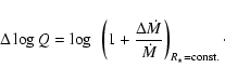 |
(10) |
Thus, before we calculate the total error in mass-loss rate which
depends on both the error in Q and in ![]() via
via
Generally, ![]() will become smaller if
will become smaller if ![]() is increased and vice
versa. In particular, we have varied
is increased and vice
versa. In particular, we have varied ![]() typically by (+0.2/-0.1) to
obtain i) a conservative lower limit for
typically by (+0.2/-0.1) to
obtain i) a conservative lower limit for ![]() and ii) to exclude
and ii) to exclude ![]() values below 0.7 (which are difficult to justify theoretically). Only in
those case where we were able to constrain
values below 0.7 (which are difficult to justify theoretically). Only in
those case where we were able to constrain ![]() due to additional
arguments (cf. Sect. 5), the "allowed range'' of
due to additional
arguments (cf. Sect. 5), the "allowed range'' of ![]() could
be (moderately) reduced. The specific values chosen for
could
be (moderately) reduced. The specific values chosen for
![]() and
and
![]() as well as the errors in
as well as the errors in ![]() estimated in such a
way are listed in Table 3. Together with the small influence of
estimated in such a
way are listed in Table 3. Together with the small influence of ![]()
![]() ,
we obtain typical uncertainties in
,
we obtain typical uncertainties in ![]()
![]() between 0.1 to 0.2
dex, i.e., of the order of 25...60%, which indicates the lower quantity of
the derived mass-loss rates if H
between 0.1 to 0.2
dex, i.e., of the order of 25...60%, which indicates the lower quantity of
the derived mass-loss rates if H
![]() is in absorption (cf. Paper I and
Kudritzki & Puls 2000).
is in absorption (cf. Paper I and
Kudritzki & Puls 2000).
For stars with extremely low mass-loss rates, where only an upper limit of
![]() could be deduced (HD 217086, HD 13268, HD 191423 and
HD 149757), the same procedure has been applied, such that the derived
limiting values,
could be deduced (HD 217086, HD 13268, HD 191423 and
HD 149757), the same procedure has been applied, such that the derived
limiting values, ![]() and
and ![]() ,
are also
only upper limits. Note the extreme uncertainty in
,
are also
only upper limits. Note the extreme uncertainty in ![]() for HD 217086 and
HD 149757.
for HD 217086 and
HD 149757.
So far, we have considered the errors for the quantities which can actually be
"measured'' from a spectroscopic analysis, i.e.,
![]() ,
,
![]() ,
,
![]() ,
Q and, to a lesser extent,
,
Q and, to a lesser extent,
![]() ,
,
![]() ,
and
,
and ![]() .
In the following, we briefly summarize the errors in the derived quantities
which are needed for our further interpretation
in order to assess the achieved accuracy. All values are presented in
Table 4.
.
In the following, we briefly summarize the errors in the derived quantities
which are needed for our further interpretation
in order to assess the achieved accuracy. All values are presented in
Table 4.
At first, the error in luminosity is given by
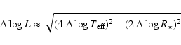 |
(12) |
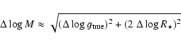 |
(13) |
Our analysis was carried out using a large sample of spectral subtypes
ranging from O2 to O9.5 enabling us to obtain a temperature scale for O
supergiants, giants, and dwarfs. Figure 9 displays our current
calibration of
![]() vs. spectral type for Galactic O-type stars. From this
plot, we conclude that the influence of line-blanketing redefines this
temperature scale significantly. Supergiants of spectral type O2 to O9.5 are
now located between roughly 43 000 K and 30 000 K (if we assume that the
effective temperature of HD 93129A is not too wrong), whereas dwarfs of
spectral type O3 to O9 are located between 47 000 K and 32 000 K.
vs. spectral type for Galactic O-type stars. From this
plot, we conclude that the influence of line-blanketing redefines this
temperature scale significantly. Supergiants of spectral type O2 to O9.5 are
now located between roughly 43 000 K and 30 000 K (if we assume that the
effective temperature of HD 93129A is not too wrong), whereas dwarfs of
spectral type O3 to O9 are located between 47 000 K and 32 000 K.
Our results indicate a somewhat larger influence of line-blocking on the effective temperature of dwarfs than found by Martins et al. (2002) in a comparable investigation utilizing model grids. Typically, our temperatures are lower by 1000 to 2000 K. One has to note, however, that a significant number of our objects are fast rotators, which might be affected by gravity darkening (e.g., Petrenz & Puls 1996; Cranmer & Owocki 1995) and hence appear cooler than their non-rotating counterparts.
Moving from dwarfs to supergiants (the temperatures of giants lie in
between), we can see that our temperature scale is somewhat hotter than the scale derived by Crowther et al. (2002, line-blanketed models using CMFGEN). The differences are marginal at spectral type O4 but
increase towards later types, where the discrepancy is of the order of 4000 K. It
should be mentioned though that the accomplished analysis and results
obtained by Crowther et al. (2002) comprised extreme Magellanic Clouds objects,
whereas in our sample such extreme objects are rare. Thus, it can be
speculated that the derived effective temperatures are lower just because of
the extreme wind-density of the objects analyzed (see below). Note also
that the lower entry at O4 corresponds to ![]() Pup. For this star (which
has a much more typical wind-density), the results of both analyses (ours
and the one performed by Crowther et al.) agree perfectly,
with a derived value for
Pup. For this star (which
has a much more typical wind-density), the results of both analyses (ours
and the one performed by Crowther et al.) agree perfectly,
with a derived value for
![]() = 39 000 K.
= 39 000 K.
![\begin{figure}
\par\includegraphics[width=8.6cm,clip]{4006.f9}
\end{figure}](/articles/aa/full/2004/07/aa4006/img254.gif) |
Figure 9:
|
| Open with DEXTER | |
Compared to the latest
![]() -spectral type calibrations published by
Vacca et al. (1996), which is based on plane-parallel, pure H/He model atmospheres,
the differences are of the order of 4000 K to 8000 K at earliest spectral
types and become minor around B0, as also shown in Fig. 9. In the
following, we will discuss the origin of these differences in
considerable detail.
-spectral type calibrations published by
Vacca et al. (1996), which is based on plane-parallel, pure H/He model atmospheres,
the differences are of the order of 4000 K to 8000 K at earliest spectral
types and become minor around B0, as also shown in Fig. 9. In the
following, we will discuss the origin of these differences in
considerable detail.
As mentioned above, the inclusion of line-blanketing effects reduces the
effective temperature scale significantly, when compared to the results from
pure H/He models without winds (and, to a lesser extent, when compared to
the results from pure H/He models with winds, cf. Herrero et al. 2002). As
we will see in the next section, the gravities become smaller as well, at
least in the typical case. On the other hand, the values for ![]() and
and ![]() remain roughly at their "old'' values, so that we can anticipate a
significantly modified wind-momentum luminosity relation, due to the
decrease in luminosity. Thus, we find severe effects concerning all problems
related to
remain roughly at their "old'' values, so that we can anticipate a
significantly modified wind-momentum luminosity relation, due to the
decrease in luminosity. Thus, we find severe effects concerning all problems
related to
![]() as function of spectral type (and luminosity class, due to
the additional impact of mass-loss), and in the following we will
investigate the question why the stars "become
cooler'' in more detail.
as function of spectral type (and luminosity class, due to
the additional impact of mass-loss), and in the following we will
investigate the question why the stars "become
cooler'' in more detail.
![\begin{figure}
\par\includegraphics[width=8.4cm,clip]{4006.f10}
\end{figure}](/articles/aa/full/2004/07/aa4006/img255.gif) |
Figure 10:
Emergent Eddington flux |
| Open with DEXTER | |
![\begin{figure}
\par\includegraphics[width=8.8cm,clip]{4006.f11}
\end{figure}](/articles/aa/full/2004/07/aa4006/img256.gif) |
Figure 11:
As Fig. 10, but for corresponding radiation
temperatures
|
| Open with DEXTER | |
Due to the presence of the multitude of metal-lines in the EUV, the flux is depressed ("blocked'') in this regime, compared to a metal-line-free model. Since the total flux, however, has to be conserved the flux blocked by the lines will emerge at other frequencies. This is the case in regions where only a few lines are present, i.e., at longer wavelengths, resulting in an increase of the optical flux.
This can readily be seen in Figs. 10 and 11, where
we compare the results from a prototypical example (our current model of
HD 15629 (O5V((f)),
![]() = 40 500 K,
= 40 500 K, ![]() = 3.7, hereafter "model 1'') with
those from a pure H/He model (with negligible wind) at the same effective
temperature and gravity ("model 2''). Note in particular that the
radiation temperature in the V-band (and close to H
= 3.7, hereafter "model 1'') with
those from a pure H/He model (with negligible wind) at the same effective
temperature and gravity ("model 2''). Note in particular that the
radiation temperature in the V-band (and close to H
![]() )
is given by
)
is given by
![]()
![]()
![]() , compared to the values of
0.75 ...0.8
, compared to the values of
0.75 ...0.8
![]() for pure H/He models (Paper I). Thus, the ratio of the emergent fluxes
longwards and shortwards from the flux maximum increases due to
line-blocking/blanketing.
for pure H/He models (Paper I). Thus, the ratio of the emergent fluxes
longwards and shortwards from the flux maximum increases due to
line-blocking/blanketing.
The process responsible for achieving this flux increase at longer
wavelengths is line-blanketing. Due to the blanket of metal-lines
above the continuum-forming layer, a significant fraction of photons is
scattered back (or emitted in the backwards direction), such that the number
density of photons (![]() mean intensity
mean intensity ![]() )
below this blanket is
larger compared to the line-free case. These photons are (partially)
thermalized, and the (electron-) temperature (around
)
below this blanket is
larger compared to the line-free case. These photons are (partially)
thermalized, and the (electron-) temperature (around
![]() )
increases. Since the emergent flux is proportional to the
source-function at
)
increases. Since the emergent flux is proportional to the
source-function at
![]() (Eddington-Barbier), and since the
NLTE-departure coefficients for the excited levels of hydrogen are close to
unity for hot stars (note that the optical continuum is dominated by
hydrogen bf-processes), an increase in temperature directly translates
into an increase of the optical flux.
(Eddington-Barbier), and since the
NLTE-departure coefficients for the excited levels of hydrogen are close to
unity for hot stars (note that the optical continuum is dominated by
hydrogen bf-processes), an increase in temperature directly translates
into an increase of the optical flux.
Thus, if we determined effective temperatures from optical continuum
fluxes (concerning the failure of such a method, see Hummer et al. 1988), the
reduction of
![]() would be easily explained:
would be easily explained:
Although the actual analysis of
Line-blanketed models of hot stars have photospheric He ionization fractions similar to those from unblanketed models at higher
The final question then is: What determines the displayed behaviour of the ionization fractions? If we concentrated in Fig. 11, this behaviour would remain unclear. In model 1, the emergent flux shortwards of the He II-Lyman-edge is lowest. In so far, we would erroneously conclude that this model has the highest population of He II (at least, regarding the ground-state), in contrast to what is displayed in Fig. 12
![\begin{figure}
\par\includegraphics[width=8.8cm,clip]{4006.f12}
\end{figure}](/articles/aa/full/2004/07/aa4006/img263.gif) |
Figure 12:
Ionization fractions of He for the different models from
Fig. 10, as function of
|
| Open with DEXTER | |
Thus, in order to understand the run of ionization, we have to consider the
mean intensity, plotted in Fig. 13 as corresponding
radiation temperature (
![]() for a depth of
for a depth of
![]() .
Most important and in contrast to Fig. 11 (emergent
flux) is the fact that the mean intensities shortwards of the He II Lyman edge are now
ordered in the following sequence (from lowest to highest values): model 2, 1 and 3,
i.e., the results for the blanketed model lie in between the results of the
unblanketed ones. This is true not only for
.
Most important and in contrast to Fig. 11 (emergent
flux) is the fact that the mean intensities shortwards of the He II Lyman edge are now
ordered in the following sequence (from lowest to highest values): model 2, 1 and 3,
i.e., the results for the blanketed model lie in between the results of the
unblanketed ones. This is true not only for
![]() ,
but also for the
complete photosphere, and it is also true for the run of the electron
temperature, lying in between the temperature stratifications for model 2
and 3 due to the effects of line-blanketing as discussed above.
,
but also for the
complete photosphere, and it is also true for the run of the electron
temperature, lying in between the temperature stratifications for model 2
and 3 due to the effects of line-blanketing as discussed above.
![\begin{figure}
\par\includegraphics[width=8.6cm,clip]{4006.f13}
\end{figure}](/articles/aa/full/2004/07/aa4006/img265.gif) |
Figure 13:
As Fig. 11, but with radiation temperatures calculated
from mean intensity |
| Open with DEXTER | |
It is well known that the ionization balance (or more correctly,
the ratio between the ground state occupation numbers of ion k and ion
k+1) can be approximated by (e.g., Abbott & Lucy 1985; Puls et al. 2000)
![\begin{figure}
\par\includegraphics[width=8.5cm,clip]{4006.f14}
\end{figure}](/articles/aa/full/2004/07/aa4006/img272.gif) |
Figure 14: As Fig. 12, but for ionization ratios He II/He III (upper panel) and He I/He III (lower panel). Both panels show the actual ratios for all three models as well as the ratios as approximated by Eq. (15), using mean intensities at the ionization edge. The offset between all four arrays of curves is arbitrary. Obviously, the approximation is a good representation for the actual situation (see text). |
| Open with DEXTER | |
Figure 15 finally displays the corresponding profiles for He I 4471. Obviously, the results for model 1 and 3 are indistinguishable,
whereas model 2 produces a much stronger profile. Thus, a spectroscopic
analysis of hot stars, based on the He ionization equilibrium and performed
by means of blanketed models, will usually result in parameters at lower
![]() and lower
and lower ![]() ,
compared to an analysis utilizing pure H/He models.
,
compared to an analysis utilizing pure H/He models.
The parameters derived from He I, of course, have to consistently produce
the other (optical) lines from hydrogen and He II. Since for hotter stars
the He II lines
![]() ,
4541 are preferentially fed by
recombination from He III (which remains the dominant ion with and without
blocking), they remain almost unaffected by temperature variations and react
mainly (but weakly) on gravity (cf. the corresponding sequence of He II lines in Fig. 8). On the other hand, the hydrogen Balmer lines remain
fairly unaltered if temperature and gravity are changed in parallel, which
needs to be done in any case if He I is to be preserved.
,
4541 are preferentially fed by
recombination from He III (which remains the dominant ion with and without
blocking), they remain almost unaffected by temperature variations and react
mainly (but weakly) on gravity (cf. the corresponding sequence of He II lines in Fig. 8). On the other hand, the hydrogen Balmer lines remain
fairly unaltered if temperature and gravity are changed in parallel, which
needs to be done in any case if He I is to be preserved.
![\begin{figure}
\par\includegraphics[width=8.5cm,clip]{4006.f15}
\end{figure}](/articles/aa/full/2004/07/aa4006/img274.gif) |
Figure 15:
He I 4471 line ( |
| Open with DEXTER | |
It is hence possible to obtain line-fits of almost equal quality from
blanketed and unblanketed models, if the former have lower
![]() and
and ![]() than the latter. For physical reasons we prefer the former, implying
that we have to accept a re-calibration of stellar parameters as a function
of spectral type.
than the latter. For physical reasons we prefer the former, implying
that we have to accept a re-calibration of stellar parameters as a function
of spectral type.
In the following we will see that there is also another possibility: If the
hydrogen lines "forbid'' a decrease in gravity, we might be able
to obtain a fit at lower
![]() and equal
and equal ![]() ,
but with a reduced helium abundance. This reduction then compensates
for the increase of the He I fraction, which otherwise could be obtained
only by a decrease in
,
but with a reduced helium abundance. This reduction then compensates
for the increase of the He I fraction, which otherwise could be obtained
only by a decrease in ![]() .
The He II lines must allow for such
a reduction, which is possible in certain domains of the (
.
The He II lines must allow for such
a reduction, which is possible in certain domains of the (
![]() ,
,
![]() )-plane.
)-plane.
From these results it becomes also clear why the
![]() correction for
supergiants is larger than for dwarfs. Supergiants have a stronger wind due
to a larger luminosity. At first glance, one might speculate that the
major effect is an increased backwarming effect due to an increased
wind-albedo (cf. Voels et al. 1989; Hummer 1982): the "blanket'' becomes denser
because of the increase in line opacity and the velocity shift in the wind.
However, in most cases this effect is minor
compared to the influence of the wind itself. In a dense wind,
the line cores are formed in the wind, and particularly He I is
significantly filled in by wind emission (Fig. 15). Thus, a
larger correction to even lower
correction for
supergiants is larger than for dwarfs. Supergiants have a stronger wind due
to a larger luminosity. At first glance, one might speculate that the
major effect is an increased backwarming effect due to an increased
wind-albedo (cf. Voels et al. 1989; Hummer 1982): the "blanket'' becomes denser
because of the increase in line opacity and the velocity shift in the wind.
However, in most cases this effect is minor
compared to the influence of the wind itself. In a dense wind,
the line cores are formed in the wind, and particularly He I is
significantly filled in by wind emission (Fig. 15). Thus, a
larger correction to even lower
![]() is required to match the observations,
compared to an analysis based on wind-free models.
is required to match the observations,
compared to an analysis based on wind-free models.
One last comment: Not only
![]() and
and ![]() have an influence on the effect
of line-blocking, but also
have an influence on the effect
of line-blocking, but also ![]() ,
particularly for dwarfs.
Since with increasing
,
particularly for dwarfs.
Since with increasing ![]() the photospheric density increases,
the recombination rates of the metal-ions become enhanced, which
results in a higher population of the lower ionization states. Less ionized
metals have a more complex level structure whose more numerous lines then
enhance the blocking and blanketing effect.
the photospheric density increases,
the recombination rates of the metal-ions become enhanced, which
results in a higher population of the lower ionization states. Less ionized
metals have a more complex level structure whose more numerous lines then
enhance the blocking and blanketing effect.
Figures 16 and 17 show the spectroscopist's view of the
Hertzsprung-Russel diagram, namely ![]() vs.
vs.
![]() ,
which is independent of
any uncertainty in the distance.
Compared to the results from Paper I, a shift towards lower temperatures can
be observed for all stars in our sample as indicated by the displacement
vectors, which is in agreement with the results from above. As shown,
we would also expect a (moderate) reduction of
,
which is independent of
any uncertainty in the distance.
Compared to the results from Paper I, a shift towards lower temperatures can
be observed for all stars in our sample as indicated by the displacement
vectors, which is in agreement with the results from above. As shown,
we would also expect a (moderate) reduction of ![]()
![]() , which is found for only 14 out of 24 sample stars.
For eight stars, the gravities remain
unaltered, and for two stars, HD 24912 and HD 207198 (luminosity class III
and I, respectively), we actually had to increase
, which is found for only 14 out of 24 sample stars.
For eight stars, the gravities remain
unaltered, and for two stars, HD 24912 and HD 207198 (luminosity class III
and I, respectively), we actually had to increase ![]() in order to obtain a
convincing fit.
in order to obtain a
convincing fit.
![\begin{figure}
\par\includegraphics[width=8.8cm,clip]{4006.f16}
\end{figure}](/articles/aa/full/2004/07/aa4006/img275.gif) |
Figure 16:
True gravity
|
| Open with DEXTER | |
![\begin{figure}
\par\includegraphics[width=8.8cm,clip]{4006.f17}
\end{figure}](/articles/aa/full/2004/07/aa4006/img278.gif) |
Figure 17:
True gravity
|
| Open with DEXTER | |
If we consider those objects in more detail where the gravity remained at its old value (or had to be increased), it turns out that for 9 of the 12 objects we derived a lower helium abundance than found by Herrero et al. (1992). These cases, thus, comprise the alternative stated above: Instead of a reduced gravity, which in these cases is "forbidden'' from the hydrogen Balmer lines, we obtained a reduced helium abundance. Therefore, the well-known helium discrepancy has considerably been reduced by our analysis using blanketed models (see also Herrero et al. 2002).
Figure 17 again displays our new ![]() vs.
vs.
![]() diagram for
Galactic O-stars, but now we compare the results to a recent calibration implicitly
provided by Markova et al. (2003), who have partly used the results described in the
present paper. In particular, the plot serves as a consistency check, because
Markova et al. derived two independent calibrations,
diagram for
Galactic O-stars, but now we compare the results to a recent calibration implicitly
provided by Markova et al. (2003), who have partly used the results described in the
present paper. In particular, the plot serves as a consistency check, because
Markova et al. derived two independent calibrations,
![]() vs. spectral type
and
vs. spectral type
and
![]() vs. spectral type. Since their calibrations are based on
a linear model (with all its caveats, particularly for extreme supergiants),
it is possible to combine both and to derive a
calibration for
vs. spectral type. Since their calibrations are based on
a linear model (with all its caveats, particularly for extreme supergiants),
it is possible to combine both and to derive a
calibration for ![]() vs.
vs.
![]() .
This is what we have done in
Fig. 17, where also the corresponding coefficients have been
tabulated as a function of luminosity class.
.
This is what we have done in
Fig. 17, where also the corresponding coefficients have been
tabulated as a function of luminosity class.
In the case of class I and III objects, also this new combination
agrees with our results: almost all objects are within the
typical error bars
![]() K and
K and
![]() ,
even if we include the "problematic'' object
HD 207198 mentioned above (this object, however, together with
,
even if we include the "problematic'' object
HD 207198 mentioned above (this object, however, together with
![]() Cep, does lie above the general trend).
Cep, does lie above the general trend).
It should be noted that some of the stars studied have deliberately been excluded from the analysis performed by Markova et al. (2003). Not only were the two binaries HD 93129A and HD 303308 discarded but also the fast rotators (e.g., HD 217086 and HD 13268).
Nevertheless, the quality of the comparison performed is rather good with
exception of the class V objects. For this luminosity class, Markova et al.
have included the results obtained by Martins et al. (2002) into their calibrations.
These results are based on an analysis of model-grids and
on a different code ( CMFGEN), which might lead to a certain
inconsistency. The comparison of our results
with the calibration now indicates a steeper relation, if we do not exclude
the "outliers'' HD 217086 and HD 15629 (both with
![]() ).
For both stars, the fit quality is very good, making an error in
the spectroscopically derived
).
For both stars, the fit quality is very good, making an error in
the spectroscopically derived ![]() very unlikely).
To account for this problem. we have added an alternative
regression based on our results only (along with the corresponding
coefficients), denoted by the long-dashed line in Fig. 17.
very unlikely).
To account for this problem. we have added an alternative
regression based on our results only (along with the corresponding
coefficients), denoted by the long-dashed line in Fig. 17.
If we assume, on the other hand, that the regression by Markova et al. were
correct, the mismatch could be
explained by means of an under-estimate of the true gravity, at least for
HD 15629 (![]() sini = 90 km s-1) in case it were a fast
rotator seen pole-on (Eq. (5)). For HD 217086, however,
this possibility can most probably be excluded, since it is a
fast rotator with only a small error in the centrifugal correction.
sini = 90 km s-1) in case it were a fast
rotator seen pole-on (Eq. (5)). For HD 217086, however,
this possibility can most probably be excluded, since it is a
fast rotator with only a small error in the centrifugal correction.
In conclusion, the ![]() vs.
vs.
![]() calibration for l.c.V objects remains
somewhat uncertain, whereas for l.c.I/III stars no obvious problems are
visible.
calibration for l.c.V objects remains
somewhat uncertain, whereas for l.c.I/III stars no obvious problems are
visible.
Figure 18 shows the position of our objects in the HR Diagram,
where different symbols have been used to mark objects with large He abundances or rotational velocities.
![\begin{figure}
\par\includegraphics[width=8.1cm,clip]{4006.f18}
\end{figure}](/articles/aa/full/2004/07/aa4006/img280.gif) |
Figure 18:
The HR diagram for our sample. Filled symbols indicate stars with
He abundances higher than
|
| Open with DEXTER | |
A comparison with the data from Paper I using the same absolute magnitudes (which would slightly modify the entries in Fig. 18) reveals two major differences which are explained by the new, lower temperatures and subsequently by the lower luminosities (remember that the radii are very similar).
First, lower masses are derived for the most massive
stars, even if we include the binary components in Carina.
In Paper I, progenitor masses in excess of 120
![]() and actual
masses in excess of 100
and actual
masses in excess of 100
![]() were derived for the most massive stars,
whereas in our present work all stars have progenitor masses and actual masses
below 100
were derived for the most massive stars,
whereas in our present work all stars have progenitor masses and actual masses
below 100
![]() .
.
Second, all of our stars are clearly separated from the ZAMS except
HD 93128, although we have another five stars classified as dwarfs. This
offset in effective temperature cannot be explained by distance
uncertainties, unless they have been seriously overestimated (which would
then pose a problem for HD 93128). A similar effect has been found in the
data set analyzed by Herrero et al. (1992), although they have used different
evolutionary models and there were no sample stars as young as HD 93128.
Investigating the evolutionary tracks, this star would have an age of
only 0.15 Myr (see also Penny et al. 1993) which is much less than the age
of the next youngest star, HD 93250 with an age of 1.3 Myr. Although the
uncertainties in the derived ages are very large, this finding is consistent
with the fact that both stars have very similar spectra and parameters
(
![]() and
and ![]() ), but almost one and a half magnitudes difference in
brightness. It is also consistent with the fact that HD 93128 is a member
of Trumpler 14, which has been argued to be significantly younger than Tr 16
to which HD 93250 belongs (see Walborn 1982a,1995).
(Aside: we would like to point out that also HD 93250 might be a binary
(cf. Walborn 1982b, but also Walborn et al. 2002)
which would additionally explain the rather
low wind-momentum rate of this star compared to similar objects.)
), but almost one and a half magnitudes difference in
brightness. It is also consistent with the fact that HD 93128 is a member
of Trumpler 14, which has been argued to be significantly younger than Tr 16
to which HD 93250 belongs (see Walborn 1982a,1995).
(Aside: we would like to point out that also HD 93250 might be a binary
(cf. Walborn 1982b, but also Walborn et al. 2002)
which would additionally explain the rather
low wind-momentum rate of this star compared to similar objects.)
From Fig. 18 we can also read off the masses predicted by the evolutionary tracks (i.e., the evolutionary masses) and compare them with those derived from the stellar parameters which were determined by spectral analysis (i.e., the spectroscopic masses). Note that both masses depend in a similar way on the adopted distance, and, therefore, their difference will not change unless we have to modify this distance dramatically.
Herrero et al. (1992) performed this comparison and found that the spectroscopic masses of giants and supergiants were systematically smaller than the evolutionary ones. At the same time, the spectroscopically determined helium over-abundances could not be explained by current theories of stellar structure and evolution. The correlation of the mass discrepancy, i.e., the difference between evolutionary and spectroscopic masses, and the distance to the Eddington limit indicated that the deduced discrepancy might have been related to the fact that Herrero et al. (1992) omitted sphericity and mass-loss in their analyses. However, even with the (approximate) inclusion of sphericity and mass-loss in the determination of stellar parameters as performed in Paper I, the actual problem could not been solved, but it could be improved.
From a recent analysis of seven Cyg OB2 supergiants including the effects of sphericity, mass-loss and line blanketing, Herrero et al. (2002) found no conclusive evidence for a mass discrepancy to be present. While the star with the lowest mass still showed a discrepancy, the other six stars were found to be evenly distributed on each side of the 1:1 line dividing spectroscopic and evolutionary mass, with the error bars crossing it.
In the present context and to illuminate the effects of line
blocking/blanketing, it is now interesting to compare the evolutionary and
spectroscopic masses from Paper I with the ones obtained in the present
analysis, using the same absolute magnitudes.
The result can be seen in Fig. 19. A distinct
improvement of the general situation is obvious, especially for a number of
stars in the "intermediate'' mass range. Not surprisingly, these are stars
for which the correction in effective temperature is very large.
![\begin{figure}
\par\includegraphics[angle=90,width=8.4cm,clip]{4006.f19}
\end{figure}](/articles/aa/full/2004/07/aa4006/img281.gif) |
Figure 19:
Evolutionary vs. spectroscopic masses obtained in
Paper I (open squares) and in the present work (filled circles), using the
same absolute magnitudes (
|
| Open with DEXTER | |
The present situation (with respect to ![]() and
and ![]() from
Table 1) is displayed in Fig. 20.
We see that for almost all stars the corresponding
error bars cross the 1:1 line with exception of those three objects with the
lowest spectroscopic mass (which are not the three objects with the
lowest luminosity in Fig. 18).
from
Table 1) is displayed in Fig. 20.
We see that for almost all stars the corresponding
error bars cross the 1:1 line with exception of those three objects with the
lowest spectroscopic mass (which are not the three objects with the
lowest luminosity in Fig. 18).
Although our new results are consistent with the ones found by Herrero et al. (2002),
implying that the mass discrepancy seems to be limited to
stars of less than 15
![]() ,
there is still additional concern. Most stars
with masses lower than 50
,
there is still additional concern. Most stars
with masses lower than 50
![]() (including those three objects with
mass discrepancy) follow an imaginary line located
parallel to the 1:1 line which is displaced by about 10
(including those three objects with
mass discrepancy) follow an imaginary line located
parallel to the 1:1 line which is displaced by about 10
![]() in ordinates.
We consider this finding as a milder
form of the original mass discrepancy which still has to be explained.
in ordinates.
We consider this finding as a milder
form of the original mass discrepancy which still has to be explained.
Unfortunately, is not possible to perform a similar comparison using
evolutionary calculations based on rotating models as presented by
Meynet & Maeder (2000) and Heger & Langer (2000), since we do not know the initial
rotational velocity of our objects.
If we simply assume that all our objects had started with 300 km s-1,
the remaining discrepancies as discussed above would still have persisted.
At least the derived range of He abundances could be explained, but
not necessarily at the correct effective
temperature, luminosity, and age as discussed by Herrero & Lennon (2003).
![\begin{figure}
\par\includegraphics[width=8.2cm,clip]{4006.f20}
\end{figure}](/articles/aa/full/2004/07/aa4006/img282.gif) |
Figure 20:
Spectroscopic and evolutionary masses
for our sample stars with data from Table 1 and errors
as discussed in Sect. 6. The binary components HD 93129A and
HD 303308 have been discarded from the plot. Open squares denote rapid rotators
with |
| Open with DEXTER | |
Whereas the effective temperatures decrease significantly, mass-loss rates
and stellar radii are hardly affected by line-blocking/blanketing and remain
roughly at their "old'' values (if the same values for distance/![]() are
used, of course). For the radii, this finding has already been
explained in Sect 7.2 (increase of
are
used, of course). For the radii, this finding has already been
explained in Sect 7.2 (increase of
![]() in the optical)
and for the mass-loss rates the argument is similar: First, the
H
in the optical)
and for the mass-loss rates the argument is similar: First, the
H
![]() -emissivity increases only weakly due to the reduced electron temperature
in the wind (at least for the hot stars considered here). Second, the
underlying continuum, i.e., the radiation temperature close to H
-emissivity increases only weakly due to the reduced electron temperature
in the wind (at least for the hot stars considered here). Second, the
underlying continuum, i.e., the radiation temperature close to H
![]() ,
remains
comparable to or hotter than the continuum of an
unblanketed model at its "older'', higher
,
remains
comparable to or hotter than the continuum of an
unblanketed model at its "older'', higher
![]() .
The combined effect of the
modified electron, radiation and effective temperature on
.
The combined effect of the
modified electron, radiation and effective temperature on ![]() can then be
approximated by Eq. (49) in Paper I, and in most cases it turns out that we should
expect a rather weak reduction in
can then be
approximated by Eq. (49) in Paper I, and in most cases it turns out that we should
expect a rather weak reduction in ![]() of the order of 10 to 20%.
of the order of 10 to 20%.
This expectation has been checked in Fig. 21, where we have
compared the modified wind-momentum rates as derived here with those
resulting from Paper I. To avoid any confusion due to changes in ![]() because of differences in
because of differences in ![]() ,
this comparison has been performed on
the basis of
,
this comparison has been performed on
the basis of
![]() (Table 1, last column), i.e., assuming
the same values for
(Table 1, last column), i.e., assuming
the same values for ![]() as in Paper I. With respect to the values for
luminosity and
as in Paper I. With respect to the values for
luminosity and
![]() as given in Tables 1 and 4,
this means that both quantities have been scaled with
as given in Tables 1 and 4,
this means that both quantities have been scaled with
![]() .
.
In contrast to our expectation from above, Fig. 21 shows
that in some cases we actually encounter an increase in ![]() .
The reason
for this behaviour is twofold. The fitted value of
.
The reason
for this behaviour is twofold. The fitted value of ![]() has decreased for a number of stars with emission lines, (e.g., for
has decreased for a number of stars with emission lines, (e.g., for ![]() Pup from 1.15 to 0.90), probably as a consequence of the somewhat modified
run of
Pup from 1.15 to 0.90), probably as a consequence of the somewhat modified
run of
![]() .
A decrease in
.
A decrease in ![]() then translates into an increase in
then translates into an increase in ![]() .
.
![\begin{figure}
\par\includegraphics[width=8.8cm,clip]{4006.f21}
\end{figure}](/articles/aa/full/2004/07/aa4006/img288.gif) |
Figure 21:
Logarithm of modified wind-momentum rate,
|
| Open with DEXTER | |
For objects with an almost purely photospheric H
![]() profile, on the other
hand (the four low luminosity stars for which we could obtain only upper
limits), this upper limit has increased due to the higher precision of the
present analysis: The approximate approach used in Paper I becomes somewhat
uncertain at (very) low mass-loss rates, mainly because it depends on an
incident boundary condition based on results from hydrostatic,
plane-parallel models. Additionally, all four objects are very fast
rotators. In Paper I, we reduced the rotational velocity from its
photospheric value to a somewhat lower, "effective'' value in order to
match the H
profile, on the other
hand (the four low luminosity stars for which we could obtain only upper
limits), this upper limit has increased due to the higher precision of the
present analysis: The approximate approach used in Paper I becomes somewhat
uncertain at (very) low mass-loss rates, mainly because it depends on an
incident boundary condition based on results from hydrostatic,
plane-parallel models. Additionally, all four objects are very fast
rotators. In Paper I, we reduced the rotational velocity from its
photospheric value to a somewhat lower, "effective'' value in order to
match the H
![]() profile. Again due to the higher precision of the present
unified approach, it turned out that such a modification is no longer
necessary, at least not for the three dwarfs (cf. Sects. 5 and 8). Keeping the nominal values of
profile. Again due to the higher precision of the present
unified approach, it turned out that such a modification is no longer
necessary, at least not for the three dwarfs (cf. Sects. 5 and 8). Keeping the nominal values of ![]() sini then increases the derived
mass-loss rates.
sini then increases the derived
mass-loss rates.
Insofar, the dilemma discussed in Paper I (What is
the reason that the modified wind-momentum rates of low-luminosity stars lie
below the average relation?) finds its natural explanation: For
the present results, this dilemma simply no longer exists, at least
if we assume that the actual mass-loss rates lie at the obtained upper limits
(where this assumption, admittedly, is rather bold.)
![\begin{figure}
\par\includegraphics[width=8.4cm,clip]{4006.f22}
\end{figure}](/articles/aa/full/2004/07/aa4006/img294.gif) |
Figure 22:
WLR for our sample, using the same |
| Open with DEXTER | |
From our findings, we conclude that for most of our objects the
ratio between mass-loss rate (and thus modified wind-momentum rate) and
luminosity has become larger compared to previous results. This becomes
particularly clear in Fig. 22, where we compare the average WLR
for Galactic supergiants and giants/dwarfs obtained in Paper I
(long-dashed, grey) with the corresponding regressions using the present
data, again for the same values of ![]() .
Note that the latter have
been performed accounting for the errors in both directions (
.
Note that the latter have
been performed accounting for the errors in both directions (
![]() and
and
![]() ,
cf. Table 4) and for their
correlation (both quantities depend on
,
cf. Table 4) and for their
correlation (both quantities depend on
![]() ), as described in
Markova et al. (2003).
), as described in
Markova et al. (2003).
Table 5:
Coefficients of the WLR obtained in the present investigation (discarding
HD 93129A and HD 303308 from the regression), compared to the results from
Paper I and the theoretical prediction by Vink et al. (2000). Entry 4 and 5
correspond to values obtained by using the "old'' absolute magnitudes
(
![]() ), entry 6 and 7 correspond to the values derived from new
ones including the results for seven Cyg OB2 stars by Herrero et al. (2002). The
last entry corresponds to the regression performed in Fig 24.
Present data has been analyzed by accounting for the errors in
both directions and their correlation, whereas
a standard least square fit has been performed for the data in Paper I (no
errors available).
), entry 6 and 7 correspond to the values derived from new
ones including the results for seven Cyg OB2 stars by Herrero et al. (2002). The
last entry corresponds to the regression performed in Fig 24.
Present data has been analyzed by accounting for the errors in
both directions and their correlation, whereas
a standard least square fit has been performed for the data in Paper I (no
errors available).
The corresponding coefficients with respect to the WLR,
Although quantitatively different, both the results presented here and in
Paper I indicate a clear separation between luminosity class I objects and
the rest, although this separation seems to have decreased regarding our new
data. The most obvious interpretation would be that the effective number of
lines driving the wind (comprised in the quantity ![]() from
Eq. 16) is a function of luminosity class. A comparison with recent
theoretical predictions (and even with older ones, cf. Fig. 25 in Paper I)
obtained by different independent approaches (Puls et al. 2003a; Vink et al. 2000; Pauldrach et al. 2003) suggests that this is not probable, since these calculations
predict a unique relation, almost coinciding with our present
regression for class III/V objects (cf. Figs. 22, 23).
from
Eq. 16) is a function of luminosity class. A comparison with recent
theoretical predictions (and even with older ones, cf. Fig. 25 in Paper I)
obtained by different independent approaches (Puls et al. 2003a; Vink et al. 2000; Pauldrach et al. 2003) suggests that this is not probable, since these calculations
predict a unique relation, almost coinciding with our present
regression for class III/V objects (cf. Figs. 22, 23).
If we now use our preferred absolute magnitudes, i.e., the values given in
Tables 1 and 4 and include the results obtained by
Herrero et al. (2002) for seven Cyg OB2 stars![]() (which should be free of errors
related to relative distances), the situation becomes even more confusing
as shown in Fig. 23 (see also Puls et al. 2003a, Fig. 3).
Although the Cyg OB2 sample consists almost exclusively of supergiants, only
the two most extreme supergiants (CygOB2#7 and #11) follow the "upper''
WLR from Fig. 22, whereas the derived wind-momenta for all other
(five) objects are consistent with our present WLR for class III/V stars.
(which should be free of errors
related to relative distances), the situation becomes even more confusing
as shown in Fig. 23 (see also Puls et al. 2003a, Fig. 3).
Although the Cyg OB2 sample consists almost exclusively of supergiants, only
the two most extreme supergiants (CygOB2#7 and #11) follow the "upper''
WLR from Fig. 22, whereas the derived wind-momenta for all other
(five) objects are consistent with our present WLR for class III/V stars.
In order to clarify this confusion and on the basis of a preliminary analysis of the present data set, Puls et al. (2003a) have suggested a scenario which we would like to briefly summarize, because in the following we will present the corresponding outcome using our results.
When plotted not as a function of luminosity class but as a
function of H
![]() profile type (Puls et al. 2003a, Fig. 4), it turned out that stars with H
profile type (Puls et al. 2003a, Fig. 4), it turned out that stars with H
![]() in emission and those with
absorption profiles (only partly filled in by wind emission) form two
distinct WLRs, respectively, where in this representation the CygOB2
objects make no exception.
in emission and those with
absorption profiles (only partly filled in by wind emission) form two
distinct WLRs, respectively, where in this representation the CygOB2
objects make no exception.
From these findings, Puls et al. (2003a) suggested that the different WLRs might
be a consequence of wind-clumping: The contribution of wind emission to the
total profile is significantly different for objects with H
![]() in absorption
compared to object with H
in absorption
compared to object with H
![]() in emission, since for the former only
contributions from the lowermost wind can be seen, whereas for the latter
the emission is due to a significant wind volume. Thus, there is the
possibility that for these objects we see the effects of a clumped wind which would mimic a higher mass-loss rate, as it is most
probably the case for Wolf-Rayet winds (e.g., Moffat & Robert 1994). With this
suggestion, we do not exclude the presence of clumping in the winds of
objects with H
in emission, since for the former only
contributions from the lowermost wind can be seen, whereas for the latter
the emission is due to a significant wind volume. Thus, there is the
possibility that for these objects we see the effects of a clumped wind which would mimic a higher mass-loss rate, as it is most
probably the case for Wolf-Rayet winds (e.g., Moffat & Robert 1994). With this
suggestion, we do not exclude the presence of clumping in the winds of
objects with H
![]() in absorption; owing to the low optical depth, however, we
simply cannot see it.
in absorption; owing to the low optical depth, however, we
simply cannot see it.
It should be mentioned that the principal presence of clumping has never
been ruled out for O-star winds; however, at least from conventional
spectrum analysis methods there was simply no indication that the H
![]() forming region was considerably clumped (see the discussion in Paper I).
During the past years, this situation has somewhat changed. Apart from recent
theoretical considerations (e.g., Feldmeier et al. 1997; Owocki & Puls 1999 and
references therein) which do not prohibit such a relatively deep-seated
clumped region, a number of additional evidence for such a scenario has been
gathered.
forming region was considerably clumped (see the discussion in Paper I).
During the past years, this situation has somewhat changed. Apart from recent
theoretical considerations (e.g., Feldmeier et al. 1997; Owocki & Puls 1999 and
references therein) which do not prohibit such a relatively deep-seated
clumped region, a number of additional evidence for such a scenario has been
gathered.
First, note that time-series analyses of He II 4686 from ![]() Pup by
Eversberg et al. (1998) have revealed "outward moving inhomogeneities'' from
regions near the photosphere out to 2
Pup by
Eversberg et al. (1998) have revealed "outward moving inhomogeneities'' from
regions near the photosphere out to 2 ![]() ,
i.e., just in the H
,
i.e., just in the H
![]() forming
region which extends typically out to 1.5 stellar radii. Although these
features are most probably different from the clumps suggested
here, these observations indicate that the lower wind is not as stationary
as previously assumed.
forming
region which extends typically out to 1.5 stellar radii. Although these
features are most probably different from the clumps suggested
here, these observations indicate that the lower wind is not as stationary
as previously assumed.
Second, our hypothesis is supported by a number of UV-analyses. Based on FUSE-observations of (L)MC-stars, both Crowther et al. (2002), Massa et al. (2003) and Hillier et al. (2003, see below) found indications that the winds might be clumped, majorly from the behaviour of the P V resonance line (if phosphorus is not strongly under-abundant, as claimed by Pauldrach et al. 1994). By comparing the results from self-consistent wind models and UV line-synthesis, Puls et al. (2003a) found that the clumping scenario is also consistent with the behaviour of the Si IV resonance line.
Most important in the present context, however, is the problem concerning
the cores of the (blue) Balmer lines discussed in Sect. 4. At least
for five out of the seven objects with H
![]() in emission, the synthetic H
in emission, the synthetic H
![]() H
H
![]() (where present) and H
(where present) and H
![]() lines formed in or close to the photosphere
show too much wind emission in their cores, and would require at least a
factor of 1.5 less mass-loss in order to be consistent with observations.
Interestingly, this behaviour has also been found for the extreme objects of
the Cyg OB2 sample analyzed by Herrero et al. (2002). This dilemma is not present for
stars with H
lines formed in or close to the photosphere
show too much wind emission in their cores, and would require at least a
factor of 1.5 less mass-loss in order to be consistent with observations.
Interestingly, this behaviour has also been found for the extreme objects of
the Cyg OB2 sample analyzed by Herrero et al. (2002). This dilemma is not present for
stars with H
![]() in absorption for which we anticipate that the derived
mass-loss rates are not contaminated by clumping effects.
in absorption for which we anticipate that the derived
mass-loss rates are not contaminated by clumping effects.
![\begin{figure}
\par\includegraphics[width=8.4cm,clip]{4006.f23}
\end{figure}](/articles/aa/full/2004/07/aa4006/img325.gif) |
Figure 23: As Fig. 22, but with the actual absolute magnitudes from Table 1 including the results for seven Cyg OB2 stars analyzed by Herrero et al. (2002) (enclosed by circles). |
| Open with DEXTER | |
In Fig. 24 we have considered the following question:
If the suggested scenario was correct, what (clumping) factor would be
required to "unify'' the different WLRs with each other and with the
theoretical predictions, respectively? To this end, we have modified the
mass-loss rates for all objects with H
![]() in emission (including the CygOB2
stars) in order to match the WLR of giants/dwarfs
as close as possible. This approach, of course, assumes that either the
clumping factor in the H
in emission (including the CygOB2
stars) in order to match the WLR of giants/dwarfs
as close as possible. This approach, of course, assumes that either the
clumping factor in the H
![]() emitting wind region is constant or that the H
emitting wind region is constant or that the H
![]() emitting volume is of similar size. The required factor with respect to
emitting volume is of similar size. The required factor with respect to ![]() turned out to be 0.44, corresponding to an (effective) clumping
factor
turned out to be 0.44, corresponding to an (effective) clumping
factor
![]() ,
which sounds reasonable and is
somewhat lower than the values inferred from (the outer regions of)
Wolf-Rayet winds.
,
which sounds reasonable and is
somewhat lower than the values inferred from (the outer regions of)
Wolf-Rayet winds.
With such a reduction we find an almost unique WLR consistent with
theoretical simulations![]() , where the
corresponding parameters are given in Table 5.
Recall that the quoted values have been "derived'' on the basis of the hypothesis that the modified wind-momentum rate is a function of luminosity
alone, independent of luminosity class. This hypothesis is strongly supported
by theoretical predictions and simulations in those cases where the WLR is
independent of stellar mass (which is the case for Galactic O-stars with
, where the
corresponding parameters are given in Table 5.
Recall that the quoted values have been "derived'' on the basis of the hypothesis that the modified wind-momentum rate is a function of luminosity
alone, independent of luminosity class. This hypothesis is strongly supported
by theoretical predictions and simulations in those cases where the WLR is
independent of stellar mass (which is the case for Galactic O-stars with ![]() close to 2/3). If this hypothesis is wrong, the derived clumping
factors might be somewhat too large.
close to 2/3). If this hypothesis is wrong, the derived clumping
factors might be somewhat too large.
![\begin{figure}
\par\includegraphics[width=8.4cm,clip]{4006.f24}
\end{figure}](/articles/aa/full/2004/07/aa4006/img328.gif) |
Figure 24:
WLR of the combined sample from Fig. 23,
|
| Open with DEXTER | |
In any case and in summary, there are strong indications that mass-loss
analyses of (at least) O-star winds utilizing H
![]() tend to overestimate the
resulting values, unless clumping is accounted for or the winds are
comparatively thin.
tend to overestimate the
resulting values, unless clumping is accounted for or the winds are
comparatively thin.
After finishing this investigation a very interesting paper by
Hillier et al. (2003) appeared which gave additional support to our hypothesis.
In this paper, two SMC O stars, AV83 (O7 Iaf+) and AV69 (OC7.5 III((f)))
have been analyzed by means of CMFGEN. Although both objects are shown
to be located at rather similar effective temperatures and luminosities
(
![]() = 5.54 and 5.62, respectively), their spectra display quite different wind
signatures, with H
= 5.54 and 5.62, respectively), their spectra display quite different wind
signatures, with H
![]() in emission for the supergiant and in absorption for
the giant. Whereas for the supergiant the mass-loss rate could be determined
precisely (
in emission for the supergiant and in absorption for
the giant. Whereas for the supergiant the mass-loss rate could be determined
precisely (![]() = 2.0
= 2.0
![]() for
for ![]() ,
neglecting clumping), the
giant's mass-loss rate could not be derived unambigously, due to the
,
neglecting clumping), the
giant's mass-loss rate could not be derived unambigously, due to the
![]() -problem discussed in Sect. 6.2. For
-problem discussed in Sect. 6.2. For
![]() mass-loss rates of
mass-loss rates of ![]() = 1.5, 0.92 and 0.32
= 1.5, 0.92 and 0.32
![]() are quoted,
respectively. Accounting for the different terminal velocities (960 km s-1 vs. 1800 km s-1 - strongly related to the different gravities), the
derived modified wind-momentum rates are quite similar if clumping is
neglected. For an assumed value of, e.g.,
are quoted,
respectively. Accounting for the different terminal velocities (960 km s-1 vs. 1800 km s-1 - strongly related to the different gravities), the
derived modified wind-momentum rates are quite similar if clumping is
neglected. For an assumed value of, e.g.,
![]() for the giant,
for the giant,
![]() for the less luminous supergiant is slightly larger,
by a factor of only 1.16.
for the less luminous supergiant is slightly larger,
by a factor of only 1.16.
On various evidence (including the behaviour of the P V line, see
above), the authors then argue that the supergiant wind is probably clumped,
and that the clumping should begin at the base of the wind! In this case,
for a best simultaneous fit of all photospheric and wind lines the mass-loss
rate becomes reduced by a factor of 0.37. Note that this number as well as
the conclusion of deep-seated clumping agrees very well with our above
hypothesis. Note also that no clumping correction has been applied to the
giant, since clumping is (if at all) only weakly visible in a small number
of UV wind lines (O IV and C IV), such that a correction of ![]() would be less than for the supergiant. Taking all numbers literally, a
"unification'' of the wind-momentum rates in the same spirit as above
(i.e., claiming an equal value of
would be less than for the supergiant. Taking all numbers literally, a
"unification'' of the wind-momentum rates in the same spirit as above
(i.e., claiming an equal value of ![]() in Eq. (16)) would
yield a value of
in Eq. (16)) would
yield a value of
![]() for
for ![]() (giant) = 1.0, which might
be somewhat low for SMC O-(super)giants (cf. Vink et al. 2001; Puls et al. 2000).
Note, however, that only a small reduction of the giant's mass-loss rate to
a value of 0.58
(giant) = 1.0, which might
be somewhat low for SMC O-(super)giants (cf. Vink et al. 2001; Puls et al. 2000).
Note, however, that only a small reduction of the giant's mass-loss rate to
a value of 0.58
![]() (corresponding to a
(corresponding to a
![]() or/and a
moderately clumping corrected mass-loss rate) would yield a much more
typical value, i.e.,
or/and a
moderately clumping corrected mass-loss rate) would yield a much more
typical value, i.e.,
![]() .
.
In this paper, we have re-analyzed the Galactic O-star sample from Paper I
by means of line-blanketed NLTE model atmospheres in order to investigate
the influence of line-blocking/blanketing on the derived stellar and wind
parameters. For our analysis and in addition to the "conventional''
strategic lines (e.g., Herrero et al. 1992), we have included a number of
He lines neighboring H
![]() to provide complementary constraints
on the fitting procedure.
to provide complementary constraints
on the fitting procedure.
The fit quality is generally good (or even very good), except for the following systematic inconsistencies:
Compared to pure H/He plane-parallel models, our new results display the
following trend:
For a given spectral type, the effective temperatures become lower along
with a reduction of either gravity or helium abundance. The reduction of
![]() is largest at earliest spectral types and for supergiants, and
decreases towards later types. At 09.5, the differences to unblanketed
analyses are small, at least for the objects from our sample. Recent work by
Crowther et al. (2002), however, indicates that extreme O-supergiants of late
spectral types have significantly lower values of
is largest at earliest spectral types and for supergiants, and
decreases towards later types. At 09.5, the differences to unblanketed
analyses are small, at least for the objects from our sample. Recent work by
Crowther et al. (2002), however, indicates that extreme O-supergiants of late
spectral types have significantly lower values of
![]() than our objects.
than our objects.
The reduction of the effective temperature scale has been explained in
Sect. 7.2 as the final consequence of UV line-blocking,
increasing both the electron temperature by line-blanketing and the mean
intensity by back-scattering in the outer photosphere where the strategic
lines are formed. As a result, line-blanketed models of hot stars have
photospheric He ionization fractions similar to those from unblanketed
models at higher
![]() and higher
and higher ![]() .
Thus, any analysis based on the He
ionization equilibrium results in lower values of
.
Thus, any analysis based on the He
ionization equilibrium results in lower values of
![]() ,
if
line-blocking/blanketing is accounted for. In those cases, where a reduction
of
,
if
line-blocking/blanketing is accounted for. In those cases, where a reduction
of ![]() is prohibited by the Balmer line wings, the helium abundance has to
be reduced instead in order to allow for a convincing fit.
is prohibited by the Balmer line wings, the helium abundance has to
be reduced instead in order to allow for a convincing fit.
On the other hand, stellar radii and mass-loss rates (and hence modified wind-momentum rates) remain roughly unaffected by line-blanketing, since the optical fluxes from line-blanketed models are similar to those from unblanketed models at their corresponding, higher effective temperatures due to flux-conservation.
After correcting for the centrifugal acceleration (where
this correction and the corresponding error has been derived in Appendix A),
we calculated the masses and compared them with previous results as well as
with evolutionary masses. Although the former mass discrepancy
(Herrero et al. 1992) becomes significantly reduced, it still seems to exist at the
lowest masses (
![]() ). For all stars with larger mass, at least
the corresponding error bars do cross the 1:1 line. Nevertheless, a
systematic trend seems to be present: For
). For all stars with larger mass, at least
the corresponding error bars do cross the 1:1 line. Nevertheless, a
systematic trend seems to be present: For
![]() ,
the
spectroscopically derived values are still lower than the masses derived
from evolutionary calculations by roughly 10
,
the
spectroscopically derived values are still lower than the masses derived
from evolutionary calculations by roughly 10
![]() .
.
In the case of the helium discrepancy, we could significantly
reduce the He abundance for a number of objects, particularly for those
where previous values were extremely large (e.g., for HD 193682
![]() has
decreased from 0.43 to 0.20). A significant fraction of our sample stars,
however, still remains over-abundant in He. For these objects, at least
the derived range in abundance is consistent with present evolutionary
tracks when rotationally induced mixing is accounted for.
has
decreased from 0.43 to 0.20). A significant fraction of our sample stars,
however, still remains over-abundant in He. For these objects, at least
the derived range in abundance is consistent with present evolutionary
tracks when rotationally induced mixing is accounted for.
One of the major implications of reduced luminosities and
almost unaltered wind-momentum rates affects the wind-momentum luminosity
relation. Previous results for O-stars (Puls et al. 1996; Kudritzki & Puls 2000) indicated a
clear separation of the WLR as function of luminosity class, where the WLR
for supergiants was found to be more or less consistent with recent
theoretical simulations which do not predict any dependence on
luminosity class. For giants and dwarfs, the WLR was located roughly 0.5
dex below that. In addition, it showed a kink towards even lower momentum
rates for objects with
![]() < 5.3 which could not be explained so far.
< 5.3 which could not be explained so far.
Regarding our new values, the separation of the WLR is still present with
one decisive difference. Now, the WLR for giants/dwarfs is consistent
with theoretical expectations and also the kink has vanished at least
if we assume that the actual mass-loss rates lie at the obtained upper
limits. On various evidence (including recent UV-analyses and the
problematic line cores of the blue Balmer lines, see above, with
additional support from a recent investigation by Hillier et al. 2003) we
have argued that the different WLRs can be unified on the basis of the
following assumptions: For those stars with H
![]() in emission, the derived
mass-loss rates are affected by clumping in the lower wind region. For stars
with H
in emission, the derived
mass-loss rates are affected by clumping in the lower wind region. For stars
with H
![]() in absorption, on the other hand, this line is formed very close
to the photosphere so clumping effects cannot disturb the analysis. This
kind of unification would then require a clumping factor of roughly 5, where
the mass-loss rates of stars with H
in absorption, on the other hand, this line is formed very close
to the photosphere so clumping effects cannot disturb the analysis. This
kind of unification would then require a clumping factor of roughly 5, where
the mass-loss rates of stars with H
![]() in emission would typically be
overestimated by a factor of 2.3. As displayed in Fig. 24, the
combined WLR is then consistent also with theory.
in emission would typically be
overestimated by a factor of 2.3. As displayed in Fig. 24, the
combined WLR is then consistent also with theory.
We have, of course, to be open to other possibilities which might explain the discrepancies found. A combined multi-spectral analysis (UV, optical, IR and radio) based on clumped wind-models and applied to large samples of stars of different spectral type should clarify these questions as well as others, e.g., the problem of wind-momenta from mid-type B-supergiants which appear to be much lower than expected (Kudritzki et al. 1999).
One of the major problems encountered in the present analysis is the uncertainty in stellar radius, which originates from uncertain distances and enters quadratically into the values for masses, luminosities and wind-momentum rates.
Since the distances to Galactic O-stars (which are important because of their "Galactic'' abundances) will probably pose a problem for the next decade(s), there are only two possibilities to overcome this uncertainty (at least indirectly). Either we consider samples much larger than the present one (with the hope that better statistics will help to obtain better constraints), or we concentrate on the analysis of O-stars (definitely) belonging to distinct clusters (with the hope that the analysis is at least intrinsically consistent).
For recent progress into direction "one'', we refer the reader to Markova et al. (2003). Regarding the second possibility, a first step has been taken by Herrero et al. (2002), although the amount of analyzed objects (seven) is not enough to obtain representative results. Observational campaigns utilizing multi-object spectroscopy like the upcoming FLAMES-project, aiming at the analysis of samples of more than hundred Extragalactic and Galactic objects, will definitely lead to a dramatic increase of our knowledge of hot, massive stars.
Acknowledgements
T.R. gratefully acknowledges financial support in form of a grant by the International Max-Planck Research School on Astrophysics (IMPRS), Garching. Many thanks especially to the anonymous referee of this paper as well as to Dr. Mark Neeser and Dr. Nevyana Markova for useful comments on the manuscript. We would also like to thank Dr. Nolan Walborn for his suggestions, especially for drawing our attention to the importance of the Lutz-Kelker effect. This work has been partially supported by the Spanish MCyT under project PNAYA 2001-0436.
 |
(A.1) |
 |
(A.2) |
The geometrical situation is sketched in Fig. A.1. We consider two
Cartesian co-ordinate systems,
![]() and (z, p, q). The
former refers to the stellar system with rotation axis
and (z, p, q). The
former refers to the stellar system with rotation axis ![]() ,
and the
latter to the one of the observer. The z-axis is directed towards the
observer, the "impact parameter''
,
and the
latter to the one of the observer. The z-axis is directed towards the
observer, the "impact parameter'' ![]() is perpendicular to the
(z,q)-plane (identical to the
is perpendicular to the
(z,q)-plane (identical to the
![]() -plane), and q is the
"height'' of the disk, perpendicular to both z and p. Thus, both planes
are tilted with respect to one another in terms of inclination i (between q and
-plane), and q is the
"height'' of the disk, perpendicular to both z and p. Thus, both planes
are tilted with respect to one another in terms of inclination i (between q and ![]() ).
).
The co-ordinates in the stellar system can be expressed in terms of
stellar co-latitude ![]() ,
azimuthal angle
,
azimuthal angle ![]() and radius r.
Any points,
and radius r.
Any points, ![]() ,
on the stellar
surface (and only those are needed for our calculation) can be
described by the following relation:
,
on the stellar
surface (and only those are needed for our calculation) can be
described by the following relation:
 |
(A.3) |
 |
(A.4) |
 |
(A.5) |
Before we consider the general case of arbitrary inclination,
we will deal with the simpler case where
![]() (i.e., the star is observed equator-on). In this case,
the stellar system (where
(i.e., the star is observed equator-on). In this case,
the stellar system (where ![]() is defined) and the
system of the observer coincide, i.e.,
is defined) and the
system of the observer coincide, i.e., ![]() ,
such that the transformation from
,
such that the transformation from ![]() to
to
![]() is the
following:
Any projected point on the stellar disk can be represented
by the corresponding physical location on the stellar sphere via
is the
following:
Any projected point on the stellar disk can be represented
by the corresponding physical location on the stellar sphere via
 |
(A.7) |
 |
(A.8) |
 |
(A.9) |
 |
(A.10) |
 |
(A.12) |
| |
= |  |
|
| = | (A.13) |
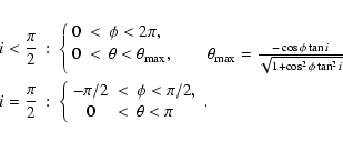
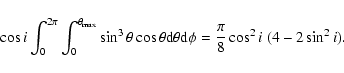 |
(A.14) |
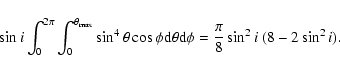 |
(A.15) |
Finally, we obtain the rather simple result
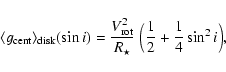 |
(A.16) |
In conclusion, the centrifugal acceleration averaged over the stellar disk
depends on two terms. The first one, constituting a minimum value, depends on
![]() alone
(which cannot be measured) and a second term depends on (
alone
(which cannot be measured) and a second term depends on (![]() sini)2
(which can be measured).
sini)2
(which can be measured).
In order to obtain a suitable approximation for the centrifugal correction
based on the measurable quantity (![]() sini)2, we will use appropriate means.
Since the probability density function for the distribution of the
inclination angle i is given by
sini)2, we will use appropriate means.
Since the probability density function for the distribution of the
inclination angle i is given by ![]() itself (see, e.g.,
Chandrasekhar & Münch 1950), the mean and standard-deviation (i.e., square-root of the
variance) of
itself (see, e.g.,
Chandrasekhar & Münch 1950), the mean and standard-deviation (i.e., square-root of the
variance) of ![]() is given by
is given by
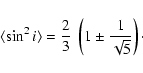 |
(A.17) |
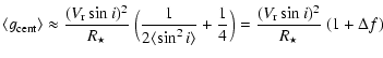 |
|||
| (A.18) |
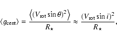
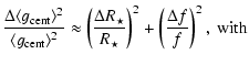
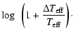
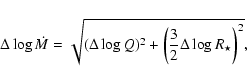
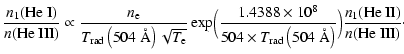
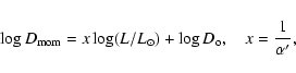
![\begin{figure}
\par\includegraphics[width=8.8cm,clip]{4006.fap}
\end{figure}](/articles/aa/full/2004/07/aa4006/img342.gif)