A&A 413, 861-878 (2004)
DOI: 10.1051/0004-6361:20031522
A. Müller - M. Camenzind
Landessternwarte Koenigstuhl, 69117 Heidelberg, Germany
Received 30 July 2003 / Accepted 22 September 2003
Abstract
Relativistic emission lines generated by thin accretion disks
around rotating black holes are an important diagnostic tool
for testing gravity near the horizon. The iron K-line is of
special importance for the interpretation of the X-ray emission
of Seyfert galaxies, quasars and galactic X-ray binary systems.
A generalized kinematic model is presented which includes radial drifts
and non-Keplerian rotations for the line emitters. The resulting
line profiles are obtained with an object-oriented ray tracer operating
in the curved Kerr background metric. The general form of the
Doppler factor is presented which includes all kinds of poloidal
and toroidal motions near the horizon. The parameters of the model
include the spin parameter, the inclination, the truncation and outer
radius of the disk, velocity profiles for rotation and radial drift,
the emissivity profile and a multi-species line-system.
The red wing flux is generally reduced when radial drift is included as
compared to the pure Keplerian velocity field.
All resulting emission line profiles can be classified as triangular,
double-horned, double-peaked, bumpy and shoulder-like. Of
particular interest are emission line profiles generated by truncated
standard accretion disks (TSD). It is also shown that the emissivity law
has a great influence on the profiles. The characteristic shoulder-like
line profile observed for the Seyfert galaxy MCG-6-30-15 can
be reproduced for suitable parameters.
Key words: galaxies: active - galaxies: Seyfert - accretion - relativity - black hole physics - line: profiles
Emission lines originating from regions where the influence of curved space-time can not be neglected are found in
accreting black hole systems like Active Galactic Nuclei (AGN), microquasars and Galactic Black Hole Candidates (GBHC).
These astrophysical systems exhibit hot plasma falling into the deep potential well of black holes. The ion species in the plasma
still have some electrons on lower shells so that there are several transitions between electron states that generate emission lines
in the X-ray range. The most prominent line is the Fe K![]() line at 6.4 keV rest frame energy (near-neutral iron). Additionally, the Fe K
line at 6.4 keV rest frame energy (near-neutral iron). Additionally, the Fe K![]() line
at 7.06 keV and rarely Ni K
line
at 7.06 keV and rarely Ni K![]() at 7.48 keV and Cr K
at 7.48 keV and Cr K![]() at 5.41 keV can be applied to fit X-ray emission line systems. The fluorescence process and its
transition energies depend on the ionization state of the species. One can distinguish hot and cold regimes of line emission which can be
described by an ionization parameter (Ballantyne et al. 2001). Generally, X-ray astronomers observe a multi-component emission line complex
of these species. The Fe K
at 5.41 keV can be applied to fit X-ray emission line systems. The fluorescence process and its
transition energies depend on the ionization state of the species. One can distinguish hot and cold regimes of line emission which can be
described by an ionization parameter (Ballantyne et al. 2001). Generally, X-ray astronomers observe a multi-component emission line complex
of these species. The Fe K![]() line dominates the line system due to its high relative strength and is often indicated in unreduced
global X-ray spectra.
line dominates the line system due to its high relative strength and is often indicated in unreduced
global X-ray spectra.
Broad X-ray emission lines originate from the hot inner parts of accreting black hole systems, typically from radii comparable to the radius of marginal stability. Naturally, these lines hint for a proximity of hot and cold material: hot material can be found in an optically thin corona, a place where cold seed photons are Comptonized to hard radiation. It is expected that the corona becomes optically thick at super-Eddington accretion rates and is dominated by Comptonization. This latter scenario seems to hold for narrow-line Seyfert-1 galaxies (NLS1s), whereas classical broad-line Seyfert-1 galaxies (BLS1s) accrete at sub-Eddington to Eddington rates.
Relatively cold material hides in the radiatively-efficient, geometrically thin and optically thick accretion disk, the so called standard disk, hereafter SSD (Shakura-Sunyaev Disk) (Shakura & Sunyaev 1973). The resulting structure equations for this standard disk have been generalized to the relativistic case later (Novikov & Thorne 1974). The hard coronal input radiation usually described by a power law illuminates the cold disk. As a consequence, the surface of the disk is ionized in a thin layer. In a fluorescence mechanism the hard radiative input is absorbed (threshold at 7.1 keV) and re-emitted in softer fluorescence photons. But in the dominant competitive process, the auger effect, the excited ions emit auger electrons and enrich the environment with hot electrons. One of the first applications of this X-ray fluorescence was performed at the microquasar Cyg X-1 (Fabian et al. 1989). These observations were supplemented by radio-quiet AGN, e.g. Seyfert galaxies, showing the same X-ray reflection signatures (Pounds et al. 1990; Tanaka et al. 1995; Reynolds & Nowak 2003).
But there are also sources exhibiting narrow X-ray emission lines. The narrow lines do not show distortion by relativistic effects. It has been proposed that narrow X-ray emission lines can be explained by reflection at the large-scale dusty torus (Turner et al. 1997). Here, the narrow line is overimposed on broad line profiles. This interpretation has been applied to some sources, like Seyfert galaxies, e.g. MCG-6-30-15 (Wilms et al. 2001), MCG-5-23-16 (Dewangan et al. 2003) and Quasars, e.g. Mrk 205 (Reeves et al. 2001).
The absence of the line feature in several Sefert-1 galaxies (Pfefferkorn et al. 2001) can be explained by global
accretion models. The first possible interpretation is that the inner edge of the disk seems to be far away from the black hole.
If the fluorescence process is still possible in that distance, the skewness of the X-ray emission line vanishes and becomes rather
Newtonian-like. In even larger distances, it is supposed that the emission line feature disappears completely because irradiation and
fluorescence is reduced. Accretion theory states that this scenario holds for low
accretion rate: then the transition radius between standard accretion disk and optically thin disk is large (Esin et al. 1997). The mass
determinations for Seyfert black holes confirm this interpretation while being in the intermediate
range of 106 to 108
![]() .
These lighter supermassive black holes seem to accrete very weakly.
.
These lighter supermassive black holes seem to accrete very weakly.
X-ray spectra of AGN and X-ray binaries are dominated by broad Comptonized continua. The properties of these spectra are discussed in the next section. The first step for astronomers is to reduce the observed data files and to extract the line profile by subtracting this global continuum emission. This procedure is already complicated because the intrinsic curvature of the Comptonized radiation is still topic of an ongoing debate.
The resulting emission line profile serves for diagnostics and to constrain essential parameters of the accreting black hole system.
So, astronomers found an X-ray imprint of black holes and can derive properties concerning the relative position from
the inner accretion disk (standard disk) to the observer, the inclination i or the rotational state of the black hole,
the Kerr rotational parameter a, the extension of the geometrically thin and optically thick standard disk, like inner radius
![]() and outer radius
and outer radius
![]() ,
the velocity field of the plasma, separated in toroidal
,
the velocity field of the plasma, separated in toroidal ![]() ,
poloidal
,
poloidal
![]() and radial
and radial ![]() components and the relative position of hot corona to cold accretion disk.
components and the relative position of hot corona to cold accretion disk.
Let us follow up the theoretical steps from black hole theory needed here until one gets simulated emission line profiles: Sect. 3 introduces the metric of rotating black holes, the Kerr geometry, and provides the standard co-ordinate system in Boyer-Lindquist form. Then, the generalized GR Doppler factor is presented. The derivation of this quantity and its signification in GR ray tracing is elaborated, too.
In Sect. 4, realistic plasma kinematics resulting from hydrodynamic and magnetohydrodynamic accretion theory is discussed. The Kerr geometry has special features that are valid independently from the accretion model! This is accessable by analytical investigations.
Another basic ingredient to calculate emission lines and spectra in general is the emissivity law that determines the
emission behaviour of the line emitting region. In Sect. 5, alternative emissivity shapes besides
th classical single power law are applied.
![\begin{figure}
\par\rotatebox{0}{\includegraphics[height=6.62cm,width=8.8cm,clip]{H4692F1.ps}}
\end{figure}](/articles/aa/full/2004/03/aah4692/img58.gif) |
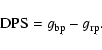
Figure 1: Prototype X-ray spectrum of a type-1 AGN (illustration idea taken from Fabian 1998). The spectrum is dominated by the global Comptonized continuum. At low energies, there is the soft excess, in principle a composition of some black bodies belonging to the disk divided into rings. At energies around 1 keV, one can recognize a complex of absorption dips, originating from the warm absorbers. The reflection component consists of a broad bump peaking around 20 keV and the prominent fluorescence emission line complex around 6.4 keV. |
| Open with DEXTER | |
Ray racing provides in a first step disk images. It may be possible to resolve these images observationally in near future. In any case, disk images as presented in Sect. 6 are very instructive unrevealing GR effects and influence of plasma dynamics.
In Sect. 7, the calculation and basic properties of the emission lines are discussed.
In the final Sect. 8, the parameter space of relativistic emission lines is investigated and suitable criteria to fix line features are presented. One can apply these criteria to observed line profiles and derive a classification in the line jungle.
The data quality increased conspicuously with the launch of the space-based X-ray observatories Chandra and XMM-Newton. The challenge in interpreting X-ray spectra of AGN and XRBs is to correctly reduce the data and subtract the continuum. Afterwards one can discuss the formation of other spectral components, such as emission lines.
X-ray spectra of Seyfert galaxies have been investigated for several years. These types of AGN were the first objects that gave
evidence for rotating black holes (Tanaka et al. 1995) and confirmed the paradigm of the AGN engine: an accreting supermassive black hole producing
high multi-wavelength luminosity. Only a few years later, high-resolution observatories allowed the
extraction of iron K emission lines in more distant objects, Quasars (Yaqoob et al. 1999). In the course of the unification scheme of AGN, the
different AGN types are considered as different evolution phases of a prototype AGN with some pecularities that mainly arise by differencies
in orientation of the accretion disk, accretion rate and black hole mass. Especially, the discrimination between Seyferts and Quasars has become
somewhat arbitrary. Only the amount of radiation, ![]()
![]() for Seyferts and 1013 to
for Seyferts and 1013 to
![]() for Quasars, is
the main difference between these two subclasses. Concerning the iron emission line feature, it can be stated that Quasars exhibit increased ionization
of the standard disk surface due to enhanced central luminosity. Therefore, weaker emission line signatures are expected (Reynolds & Nowak 2003).
for Quasars, is
the main difference between these two subclasses. Concerning the iron emission line feature, it can be stated that Quasars exhibit increased ionization
of the standard disk surface due to enhanced central luminosity. Therefore, weaker emission line signatures are expected (Reynolds & Nowak 2003).
The dichotomy phenomenon caused by disk orientation and dust torus obscuring, a generalization that can be applied to Seyferts and Quasars, is well-known: one can distinguish type-1 (low inclination) and type-2 AGN (high inclination). Hence, it is for observational reasons only possible to study relativistic emission lines of AGN of type 1.
X-ray spectra of Seyfert galaxies in the range from 0.1 to several 100 keV show many features as illustrated in Fig. 1:
overlaying the complete X-ray range there is a continuum originating from Comptonized radiation. This is the direct radiation that
reaches the observer coming from a hot corona (
![]() keV). The photon number flux per unit energy is usually modelled with a power
law distribution,
keV). The photon number flux per unit energy is usually modelled with a power
law distribution,
![]() .
The soft input radiation from the cold accretion disk is
reprocessed via unsaturated inverse Compton scattering by ultra-relativistic electrons in the corona.
Figure 2 depicts in a
simple way one probable geometry of an accreting black hole systems that hold especially for AGN and microquasars, known as "sphere+disk
geometry''. Matter has angular momentum and therefore spirales down in a flat and cold standard disk. The argument for the
flatness is because of vertical collapse due to efficient radiation cooling. The relative scale heigth H/r of these standard disks
is only 10-3 (Shakura & Sunyaev 1973). The matter within this cold disk emits a multi-color blackbody
spectrum. This is simply the superposition of a sequence of Planck spectra, e.g. rings each with a temperature
.
The soft input radiation from the cold accretion disk is
reprocessed via unsaturated inverse Compton scattering by ultra-relativistic electrons in the corona.
Figure 2 depicts in a
simple way one probable geometry of an accreting black hole systems that hold especially for AGN and microquasars, known as "sphere+disk
geometry''. Matter has angular momentum and therefore spirales down in a flat and cold standard disk. The argument for the
flatness is because of vertical collapse due to efficient radiation cooling. The relative scale heigth H/r of these standard disks
is only 10-3 (Shakura & Sunyaev 1973). The matter within this cold disk emits a multi-color blackbody
spectrum. This is simply the superposition of a sequence of Planck spectra, e.g. rings each with a temperature ![]() .
The innermost ring
is the hottest one,
.
The innermost ring
is the hottest one,
![]() .
The accretion rate determines the transition radius and this one fixes the
temperature of the inner edge of the disk. At high accretion rates, the inner edge is significantly hot so that a soft excess can be observed around 1 keV. At small accretion rates the soft excess lacks (Esin et al. 1997). The cold and thin accretion disk delivers the soft seed photons that are Comptonized
in the hot, optically thin corona. The topology of the corona is still one of the essential open questions in X-ray spectroscopy. Different
assumptions such as slab and patchy corona models have been made (Reynolds & Nowak 2003). The observed hard spectra suggest rather "sphere+disk geometries'' because
slab and patchy corona models are more efficiently radiative-cooled by seed photons from the cold disk. The reverberation mapping technique may enlighten
the spatial position of corona to accretion disk. Theoretically, it will be task of upcoming relativistic MHD simulations to unreveal the corona-disk
geometry depending on accretion rate and radiative cooling. Apparently, it turns out that the coronal emissivity is significantly enhanced at the inner edge of the standard disk (Merloni & Fabian 2003) and
that MHD dissipation plays a crucial role to invalidate the zero-torque boundary condition. Then, magnetically-induced torques at radii comparable to
the radius of marginal stability are expected to increase dissipation. This mechanism may provide the higher disk emissivities
.
The accretion rate determines the transition radius and this one fixes the
temperature of the inner edge of the disk. At high accretion rates, the inner edge is significantly hot so that a soft excess can be observed around 1 keV. At small accretion rates the soft excess lacks (Esin et al. 1997). The cold and thin accretion disk delivers the soft seed photons that are Comptonized
in the hot, optically thin corona. The topology of the corona is still one of the essential open questions in X-ray spectroscopy. Different
assumptions such as slab and patchy corona models have been made (Reynolds & Nowak 2003). The observed hard spectra suggest rather "sphere+disk geometries'' because
slab and patchy corona models are more efficiently radiative-cooled by seed photons from the cold disk. The reverberation mapping technique may enlighten
the spatial position of corona to accretion disk. Theoretically, it will be task of upcoming relativistic MHD simulations to unreveal the corona-disk
geometry depending on accretion rate and radiative cooling. Apparently, it turns out that the coronal emissivity is significantly enhanced at the inner edge of the standard disk (Merloni & Fabian 2003) and
that MHD dissipation plays a crucial role to invalidate the zero-torque boundary condition. Then, magnetically-induced torques at radii comparable to
the radius of marginal stability are expected to increase dissipation. This mechanism may provide the higher disk emissivities
![]() as recently observed in Seyfert galaxy MCG-6-30-15 (Wilms et al. 2001).
as recently observed in Seyfert galaxy MCG-6-30-15 (Wilms et al. 2001).
Here it is assumed that the corona is almost identical with an advection-dominated torus that forms by feeding from the standard disk. An alternative may
be the quasi-spherical rather Bondi-accreting Advection-Dominated Accretion Flow (ADAF) (Narayan & Yi 1994) that forms under other circumstances in accretion
theory, e.g. depending on the accretion rate. The transition region where the standard disk adjoins the hot torus is unstable. Hot corona and cold disk
may constitute a sandwich configuration where the inner edge of the cold disk oscillates in radial direction (Gracia 2003). This ADAF-SSD transition region seems to
depend on the efficiency of different cooling channels as can be found in hydrodynamic simulations (Manmoto & Kato 2000; Gracia 2002).
More recent pseudo-Newtonian hydrodynamic simulations incorporating radiation cooling via synchrotron radiation, bremsstrahlung and
Comptonization with the consideration of conduction in a two-component plasma suggest disk truncation (Hujeirat & Camenzind 2000). This means
that the accretion disk can cut off even at radii larger than the radius of marginal stability,
![]() .
Truncation of standard disks
(TSD) in general softens the argument for observed evidences of rapidly spinning black holes. This is because truncated disks do not extend to
.
Truncation of standard disks
(TSD) in general softens the argument for observed evidences of rapidly spinning black holes. This is because truncated disks do not extend to
![]() inwardly. However the decreasing
inwardly. However the decreasing
![]() for faster spinning black holes was always the argument for evidence of Kerr black
holes (Iwasawa et al. 1996).
for faster spinning black holes was always the argument for evidence of Kerr black
holes (Iwasawa et al. 1996).
![\begin{figure}
\par\rotatebox{0}{\includegraphics[height=4.8cm,width=8.8cm,clip]{H4692F2.ps}}
\end{figure}](/articles/aa/full/2004/03/aah4692/img68.gif) |
Figure 2: Illustration of topological elements in the innermost region of accreting black hole systems. The size and morphology of these elements depend on accretion rate, black hole mass and radiative cooling. |
| Open with DEXTER | |
Particularly, the cooling time-scale of synchrotron radiation is typically in the millisecond domain and cools very fast the hot accretion flow. The
Truncated Disk - Advective Torus (TDAT) scenario (Hujeirat & Camenzind 2000) produces a hot inner torus that is not stable either. It is destablized by accretion and
matter free-falls into the black hole. But a small fraction of matter can escape the black hole and is transported along magnetic field lines in polar
regions. This drives outflows that consist of disk winds on one hand and of ergospheric Poynting fluxes on the other hand. This outflow is supposed to
feed the large-scale jets of AGN or the blobs of microquasars. In a unified view, the total accretor mass, M, and the total mass accretion rate,
![]() ,
are strongly favoured to determine the spectral state and the jet injection rate and the continuity of the outflow. Relativistic emission
lines may serve as a diagnostic tool to fix these parameters.
,
are strongly favoured to determine the spectral state and the jet injection rate and the continuity of the outflow. Relativistic emission
lines may serve as a diagnostic tool to fix these parameters.
![\begin{figure}
\par\rotatebox{0}{\includegraphics[height=5.09cm,width=8.8cm,clip]{H4692F3.ps}}
\end{figure}](/articles/aa/full/2004/03/aah4692/img70.gif) |
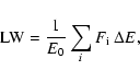
Figure 3: Radial behaviour of the Boyer-Lindquist functions at extreme Kerr (a=1.0) in the equatorial plane. Relativistic units were used. |
| Open with DEXTER | |
The continuum of the hot corona reveals an intrinsical curvature and cuts off at the high-energy branch at several hundreds of keV. The cut-off at
![]() indicates the plasma temperature in the corona (Rybicki & Lightman 1979). At the low energy branch, some sources show a soft excess with a bumpy profile.
This can be identified with a multi-color blackbody originating from the cold Compton-thick accretion disk. At 1.0 keV there is a complex structure of
warm absorbers, typically a combination of adjacent absorption edges of a variety of species
(C V, O VII, O VIII,
Ne IX etc.). These dips and their potentially relativistic broadening are still topic of an ongoing debate (Lee 2001; Mason et al. 2003).
The reflection component consists of a system of emission lines, most prominently the iron K
indicates the plasma temperature in the corona (Rybicki & Lightman 1979). At the low energy branch, some sources show a soft excess with a bumpy profile.
This can be identified with a multi-color blackbody originating from the cold Compton-thick accretion disk. At 1.0 keV there is a complex structure of
warm absorbers, typically a combination of adjacent absorption edges of a variety of species
(C V, O VII, O VIII,
Ne IX etc.). These dips and their potentially relativistic broadening are still topic of an ongoing debate (Lee 2001; Mason et al. 2003).
The reflection component consists of a system of emission lines, most prominently the iron K![]() at 6.4 keV typically, and a
broad bump peaking at 20 to 30 keV. The reflection bump is a consequence of hard radiation from the corona hitting the cold accretion disk
that is then reflected to the observer (Reynolds 1996). The origin of the iron K
at 6.4 keV typically, and a
broad bump peaking at 20 to 30 keV. The reflection bump is a consequence of hard radiation from the corona hitting the cold accretion disk
that is then reflected to the observer (Reynolds 1996). The origin of the iron K![]() line is well understood: at typical temperatures of 105 to 107 keV in the inner accretion disk, iron is ionized but not completely stripped; the K- and L-shell are still populated. First, iron is excitied
by photo-electric absorption. The threshold lies at
line is well understood: at typical temperatures of 105 to 107 keV in the inner accretion disk, iron is ionized but not completely stripped; the K- and L-shell are still populated. First, iron is excitied
by photo-electric absorption. The threshold lies at ![]() 7.1 keV so that only hard X-ray photons from the corona can release this primary process.
Then, there are two competing processes: the dominant process (66% probability) is the Auger effect where the excitation energy is emitted with an
Auger electron. This mechanism is non-radiative and enriches the disk plasma with electrons. The second and here essential process is fluorescence
(34% probability): one electron of the L-shell undergoes the transition to the K-shell accompanied by the emission of the iron K
7.1 keV so that only hard X-ray photons from the corona can release this primary process.
Then, there are two competing processes: the dominant process (66% probability) is the Auger effect where the excitation energy is emitted with an
Auger electron. This mechanism is non-radiative and enriches the disk plasma with electrons. The second and here essential process is fluorescence
(34% probability): one electron of the L-shell undergoes the transition to the K-shell accompanied by the emission of the iron K![]() fluorescence photon with 6.4 keV rest frame energy
fluorescence photon with 6.4 keV rest frame energy![]() . The emission line energy and the existence of the fluorescence line in
general depend on the ionization state of the material (Ross et al. 1999).
. The emission line energy and the existence of the fluorescence line in
general depend on the ionization state of the material (Ross et al. 1999).
The significance of other elements contributing to the reflection component is rather low, because the abundance, relative strength and fluorescence yield is low
compared to that of iron (Reynolds 1996). At most, the iron K![]() at 7.06 keV or nickel at 7.48 keV (Wang et al. 1999) and chromium at 5.41 keV could contribute
marginally. Besides, the accretion disk has only a thin ionization layer. The line producing layer has only the depth of 0.1 to 1% of the disk
thickness (Matt et al. 1997). Therefore the contributions of ionized iron from deeper regions - or even a radiation transfer problem from lower ionized
slabs - can be neglected due to high optical depths.
at 7.06 keV or nickel at 7.48 keV (Wang et al. 1999) and chromium at 5.41 keV could contribute
marginally. Besides, the accretion disk has only a thin ionization layer. The line producing layer has only the depth of 0.1 to 1% of the disk
thickness (Matt et al. 1997). Therefore the contributions of ionized iron from deeper regions - or even a radiation transfer problem from lower ionized
slabs - can be neglected due to high optical depths.
The Kerr metric describes rotating uncharged black holes. This vacuum solution of the Einstein field equations (Kerr 1963) generalizes the static
Schwarzschild solution. The line element fullfills the standard form of stationary and axisymmetric space-times
 |
(1) |
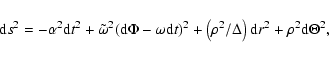 |
(2) |
The Boyer-Lindquist co-ordinates are pseudo-spherical. The expressions above are called frame-dragging frequency or potential for angular
momentum ![]() ,
cylindrical radius
,
cylindrical radius
![]() ,
lapse function or redshift factor
,
lapse function or redshift factor ![]() and some geometrical functions
and some geometrical functions ![]() and
and ![]() .
.
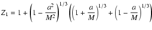
The rotation of the black hole can be parametrized by its specific angular momentum a, the so called Kerr parameter. Relativistic units
G=M=c=1 are used unless otherwise stated. Then, the natural length-scale is the gravitational radius,
![]() ,
and a varies
between -1 and 1. The interval
,
and a varies
between -1 and 1. The interval
![]() involves retrograde rotation between black hole and disk,
the interval
involves retrograde rotation between black hole and disk,
the interval ![]() means prograde rotation. From black hole theory, it is generally possible that a takes all values in this interval, but
accretion theory suggests that there is mainly one type of black holes: rotating Kerr black holes near its maximum rotation (
means prograde rotation. From black hole theory, it is generally possible that a takes all values in this interval, but
accretion theory suggests that there is mainly one type of black holes: rotating Kerr black holes near its maximum rotation (
![]() ).
This is because black holes of mass M are spun up to
).
This is because black holes of mass M are spun up to
![]() by accreting a mass
by accreting a mass ![]() .
At least the supermassive
black holes in AGN that accrete for long times are expected to rotate very rapidly,
.
At least the supermassive
black holes in AGN that accrete for long times are expected to rotate very rapidly, ![]() .
It is possible to extract angular momentum from black
holes via Blandford-Znajek (Blandford & Znajek 2000) and Penrose processes (Penrose & Floyd 1971). But these effects may not be efficient enough to slow down the black hole rotation significantly.
.
It is possible to extract angular momentum from black
holes via Blandford-Znajek (Blandford & Znajek 2000) and Penrose processes (Penrose & Floyd 1971). But these effects may not be efficient enough to slow down the black hole rotation significantly.
Figure 3 illustrates the radial dependence of the Boyer-Lindquist functions in the equatorial plane (
![]() )
at the maximum value of
black hole rotation, a=1. One can see the frame-dragging frequency
)
at the maximum value of
black hole rotation, a=1. One can see the frame-dragging frequency ![]() that increases significantly at smaller radii and reaches
that increases significantly at smaller radii and reaches
![]() in relativistic units at the horizon. This behaviour shows that dragging of inertial frames is
important when reaching the ergosphere. Another essential feature is the steep decrease of the redshift factor
in relativistic units at the horizon. This behaviour shows that dragging of inertial frames is
important when reaching the ergosphere. Another essential feature is the steep decrease of the redshift factor ![]() .
This is mainly the cause
that emission is strongly suppressed when the distance becomes smaller than approximatly the radius of marginal stability,
.
This is mainly the cause
that emission is strongly suppressed when the distance becomes smaller than approximatly the radius of marginal stability,
![]() ,
which satisfies
,
which satisfies
| (9) | |||
 |
|||
 |
Our object-oriented code KBHRT (Kerr Black Hole Ray Tracer) (Müller 2000) programmed in C++ is used to derive in the first step the image of a relativistic disk and in the second step to calculate the line flux by integrating over this image and weighting with the relativistic generalized Doppler factor and the radial disk emissivity profile. The imaging of the disk is not observationally possible because one can not (yet) resolve these distant accreting black hole systems. But these images show nicely the influence of curved space-time on photon paths. The flux is indeed the observationally accessible information and can be determined afterwards.
The code which is based on a C-code (Fanton et al. 1997) calculates the photon path by integrating the GR geodesics equation using the complete set of integrals of
motion. Besides the canonical conservative quantities like mass, energy and angular momentum, the Kerr geometry exhibits a fourth one: the Carter
constant (Carter 1968). This quantity is associated with the radial and poloidal photon momentum. The second order null geodesics equation reduces by means
of these four conservatives to a set of four first order ordinary differential equations which can easily be integrated via elliptical integrals or
Runge-Kutta schemes. The code is very fast because the position on the disk (r, ![]() ,
,
![]() )
is folded directly onto the observers screen (x, y)
without following the path stepwise between these two 2D objects (see Fig. 4). This is an alternative to the first historical method
using transfer functions (Cunningham 1975) which is still in use (Speith et al. 1995; Bromley et al. 1997) or direct shooting, a method that follows the complete ray from
locus of emission to observer.
The constraint of dealing only with flat disks that lay infinitely thin in the equatorial plane is a good approximation to the vertical collapsed
geometrically thin standard disks, however it is a restriction of our code. One recent issue shows the direction of future work, where the ray
tracing code has to be coupled to hydrodynamical or MHD accretion models (Armitage & Reynolds 2003). This coupling allows to study the variable emission near
black holes.
)
is folded directly onto the observers screen (x, y)
without following the path stepwise between these two 2D objects (see Fig. 4). This is an alternative to the first historical method
using transfer functions (Cunningham 1975) which is still in use (Speith et al. 1995; Bromley et al. 1997) or direct shooting, a method that follows the complete ray from
locus of emission to observer.
The constraint of dealing only with flat disks that lay infinitely thin in the equatorial plane is a good approximation to the vertical collapsed
geometrically thin standard disks, however it is a restriction of our code. One recent issue shows the direction of future work, where the ray
tracing code has to be coupled to hydrodynamical or MHD accretion models (Armitage & Reynolds 2003). This coupling allows to study the variable emission near
black holes.
![\begin{figure}
\par\rotatebox{0}{\includegraphics[height=4.82cm,width=8.8cm,clip]{H4692F4.ps}}
\end{figure}](/articles/aa/full/2004/03/aah4692/img104.gif) |
Figure 4: Schematical representation of a Kerr ray tracer. The light rays start at the screen ( back tracking) and hit the disk surface in the equatorial plane. On the screen the lensed image is formed as seen by a distant observer. Our solver folds directly from equatorial plane to screen. |
| Open with DEXTER | |
The KBHRT code encapsulates all relevant tools to visualize relativistic disks and emission lines. One can study the distribution of the generalized Doppler factor allover the disk or the emission itself.
The generalized Doppler factor is defined by
 |
(10) |
| |
= | ||
| = | (11) |
| |
= | ||
| = | ![$\displaystyle \gamma\left[\frac{1}{\alpha}(1-\omega\lambda)-v^{\rm (r)}\frac{\s...
...c{\sqrt{\Theta}}{\rho}-v^{\rm (\Phi)}\frac{\lambda}{\tilde{\omega}}\right]\cdot$](/articles/aa/full/2004/03/aah4692/img117.gif) |
(12) |
![\begin{displaymath}\frac{\mathcal{R}_{\rm0}}{E^{2}}=r^{4}+(a^{2}-\lambda^{2}-\ma...
...}+2\left[\mathcal{C}+(\lambda-a)^{2}\right]r-a^{2}\mathcal{C}.
\end{displaymath}](/articles/aa/full/2004/03/aah4692/img128.gif) |
(14) |
 |
(17) |
 |
(18) |
![\begin{figure}
\par\rotatebox{0}{\includegraphics[height=6.9cm,width=8.8cm,clip]{H4692F5.ps}}
\end{figure}](/articles/aa/full/2004/03/aah4692/img136.gif) |
Figure 5:
Simulated disk image at inclination of
|
| Open with DEXTER | |
In Fig. 5, the simulated distribution of the Doppler factor g from Eq. (13) on a disk with parameters typical
for Seyfert-1 galaxies (
![]() )
is shown. First, one discovers the usual separation in blueshifted and redshifted segments due to rotation of the disk.
The left-to-right symmetry is compared to the
Newtonian case distorted. The left side of the disk rotates towards the observer and this radiation is beamed due to special relativistic effects:
the matter rotation velocity becomes comparable to the speed of light. This fact can be derived from Fig. 6, illustrating the prograde and
retrograde velocity component,
)
is shown. First, one discovers the usual separation in blueshifted and redshifted segments due to rotation of the disk.
The left-to-right symmetry is compared to the
Newtonian case distorted. The left side of the disk rotates towards the observer and this radiation is beamed due to special relativistic effects:
the matter rotation velocity becomes comparable to the speed of light. This fact can be derived from Fig. 6, illustrating the prograde and
retrograde velocity component,
![]() ,
in the ZAMO frame. The Keplerian profile of
,
in the ZAMO frame. The Keplerian profile of
![]() holds only until reaching the radius of marginal
stability,
holds only until reaching the radius of marginal
stability,
![]() .
For smaller radii, one has to model this velocity component. The simplest way is to assume free-falling matter. In Fig. 6
the drift radius starts already at
.
For smaller radii, one has to model this velocity component. The simplest way is to assume free-falling matter. In Fig. 6
the drift radius starts already at
![]() .
Then the test particle falls on geodesics onto the black hole. The velocity field is a complicated
superposition of
.
Then the test particle falls on geodesics onto the black hole. The velocity field is a complicated
superposition of
![]() and
and
![]() .
Besides, the plot depicts that the component
.
Besides, the plot depicts that the component
![]() as observed by the ZAMO reaches a magnitude that is comparable to the speed of light: symmetrically in both cases, prograde and retrograde rotation, the maximum rotation velocity
is about 0.4c! Additionally, in both cases, at the horizon, this velocity component drops down to zero.
as observed by the ZAMO reaches a magnitude that is comparable to the speed of light: symmetrically in both cases, prograde and retrograde rotation, the maximum rotation velocity
is about 0.4c! Additionally, in both cases, at the horizon, this velocity component drops down to zero.
For completeness, the distribution of g down to the event horizon of the black hole is calculated to illustrate mainly the effect of gravitational
redshift. Certainly, a disk that touches the horizon is unphysical and would not be stable, unless in the case of maximum Kerr, a=1.0, where all
characteristic black hole radii coincide to
![]() .
Near the horizon the g-factor (Eq. (13)) significantly drops
down and vanishes at the horizon itself (or equivalently, the redshift z becomes infinity): the curvature of the black hole grasps everything
that is near, even light.
Figure 7 now shows the Doppler factor to the fourth power. In our approach, this is an essential ingredient for any emission
originating from the vicinity of a black hole (ray tracing using transfer functions has a weight to the third power after all). This weight to the
fourth power shows the relevance of the generalized Doppler factor. The g-factor significantly decreases inwards and becomes zero at the event horizon.
The g-factor to the fourth power shows therefore a dramatic tininess around the black hole. This feature
is called the central shadow of the black hole (Falcke et al. 2000). Likewise, one remarks a very bright region on the approaching part of the
disk (beaming). For midly and highly inclined disks there is a chance to measure this clear brightness step, e.g. with sub-mm VLBI in the Galactic Center.
This may be a method to prove the existence of the supermassive black hole with
.
Near the horizon the g-factor (Eq. (13)) significantly drops
down and vanishes at the horizon itself (or equivalently, the redshift z becomes infinity): the curvature of the black hole grasps everything
that is near, even light.
Figure 7 now shows the Doppler factor to the fourth power. In our approach, this is an essential ingredient for any emission
originating from the vicinity of a black hole (ray tracing using transfer functions has a weight to the third power after all). This weight to the
fourth power shows the relevance of the generalized Doppler factor. The g-factor significantly decreases inwards and becomes zero at the event horizon.
The g-factor to the fourth power shows therefore a dramatic tininess around the black hole. This feature
is called the central shadow of the black hole (Falcke et al. 2000). Likewise, one remarks a very bright region on the approaching part of the
disk (beaming). For midly and highly inclined disks there is a chance to measure this clear brightness step, e.g. with sub-mm VLBI in the Galactic Center.
This may be a method to prove the existence of the supermassive black hole with
![]() (Schödel et al. 2002) associated with the source Sgr A* by its radio emission. In near future, direct imaging of black holes may be possible!
(Schödel et al. 2002) associated with the source Sgr A* by its radio emission. In near future, direct imaging of black holes may be possible!
![\begin{figure}
\par\rotatebox{0}{\includegraphics[height=6cm,width=8.8cm,clip]{H4692F6.ps}}
\end{figure}](/articles/aa/full/2004/03/aah4692/img141.gif) |
Figure 6:
Radial dependence of the velocity component
|
| Open with DEXTER | |
![\begin{figure}
\par\rotatebox{0}{\includegraphics[height=7.63cm,width=8.8cm,clip]{H4692F7.ps}}
\end{figure}](/articles/aa/full/2004/03/aah4692/img144.gif) |
Figure 7:
Distribution of the Doppler factor g4 over the disk. The inner disk edge touches at
|
| Open with DEXTER | |
The generalized Doppler factor g depends on the plasma motions
(here written in the ZAMO frame),
![]() .
The usual issue forgets
about the radial and poloidal components and derives line profiles
from emitting plasma with only Keplerian motion, i.e.
pure rotation. Recent non-radiative 3D-MHD
pseudo-Newtonian simulations (Balbus & Hawley 2002) again confirm this inflow and, additionally, the poloidal motion
of disk winds. Therefore a more complicated plasma kinematics near the event horizon of Kerr black holes
is investigated in this section. The behaviour of the velocity components
.
The usual issue forgets
about the radial and poloidal components and derives line profiles
from emitting plasma with only Keplerian motion, i.e.
pure rotation. Recent non-radiative 3D-MHD
pseudo-Newtonian simulations (Balbus & Hawley 2002) again confirm this inflow and, additionally, the poloidal motion
of disk winds. Therefore a more complicated plasma kinematics near the event horizon of Kerr black holes
is investigated in this section. The behaviour of the velocity components
![]() ,
,
![]() and
and
![]() at the horizon is presented in detail below.
at the horizon is presented in detail below.
The radial velocity component will be determined by the accretion process. In this paper, it is considered that the radial drift starts
at a certain radius, the truncation radius ![]() ,
that can even be greater than the radius for marginal stability
,
that can even be greater than the radius for marginal stability
![]() .
Truncation is an essential feature of radiative accretion theory. This is motivated by radiative hydrodynamical accretion models of Hujeirat & Camenzind (2000),
discussed in Sect. 2. The correct free-fall behaviour in the Kerr geometry starting at radius
.
Truncation is an essential feature of radiative accretion theory. This is motivated by radiative hydrodynamical accretion models of Hujeirat & Camenzind (2000),
discussed in Sect. 2. The correct free-fall behaviour in the Kerr geometry starting at radius ![]() can be
studied by introducing the radial velocity component
can be
studied by introducing the radial velocity component
![]() is in a normalized ZAMO frame (indicated by round brackets)
is in a normalized ZAMO frame (indicated by round brackets)
 |
(21) |
This provides the radial drift
| (26) | |||
A realistic approach to model the radial drift is to fix the
conservatives E and J when reaching the truncation radius ![]() with the values that they take at this radius.
Then, the particle will fall freely into the black hole. The disk is
truncated at
with the values that they take at this radius.
Then, the particle will fall freely into the black hole. The disk is
truncated at
![]() ,
the truncation radius
gives the conservatives,
,
the truncation radius
gives the conservatives,
![]() and
and
![]() .
Otherwise, the
radius of marginal stability fixes the conservatives to
.
Otherwise, the
radius of marginal stability fixes the conservatives to
![]() and
and
![]() .
.
![\begin{figure}
\par\rotatebox{0}{\includegraphics[height=4.96cm,width=8.8cm,clip]{H4692F8.ps}}
\end{figure}](/articles/aa/full/2004/03/aah4692/img172.gif) |
Figure 8:
Distribution of specific angular momentum,
|
| Open with DEXTER | |
![\begin{figure}
\par\rotatebox{0}{\includegraphics[height=5.26cm,width=8.8cm,clip]{H4692F9.ps}}
\end{figure}](/articles/aa/full/2004/03/aah4692/img173.gif) |
Figure 9:
Radial distribution of prograde (solid curve),
|
| Open with DEXTER | |
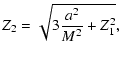
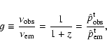
It is not possible to give arbitrary values for
constant
![]() ,
that means to fix arbitrary
,
that means to fix arbitrary ![]() .
As has been
discussed in torus solutions on the Kerr geometry (Abramowicz et al. 1978),
there is only an allowed interval of
.
As has been
discussed in torus solutions on the Kerr geometry (Abramowicz et al. 1978),
there is only an allowed interval of
![]() for the specific angular momentum, where ms denotes the
orbit of marginal stability and mb the marginally bound orbit.
This allowed interval
for the specific angular momentum, where ms denotes the
orbit of marginal stability and mb the marginally bound orbit.
This allowed interval
![]() is depicted
in Fig. 8 for a Kerr parameter of a=0.8. The general distribution
of the specific angular momentum in the Kerr geometry is represented by the curve.
The drift radius has to be chosen so that its according specific angular momentum,
is depicted
in Fig. 8 for a Kerr parameter of a=0.8. The general distribution
of the specific angular momentum in the Kerr geometry is represented by the curve.
The drift radius has to be chosen so that its according specific angular momentum,
![]() ,
just lays inbetween the two horizontal lines. These lines belong to the specific angular momenta
at the radius of marginal stability,
,
just lays inbetween the two horizontal lines. These lines belong to the specific angular momenta
at the radius of marginal stability,
![]() ,
and at the marginally bound radius,
,
and at the marginally bound radius,
![]() .
The physical reason for this restriction is, that
.
The physical reason for this restriction is, that ![]() satisfies the condition
satisfies the condition
 |
(28) |
Let us now consider the toroidal velocity component,
![]() .
From the Carter momenta it follows that
.
From the Carter momenta it follows that
 |
(31) |
 |
(32) |
![\begin{displaymath}\frac{\Theta}{E^{2}}=\frac{\mathcal{C}}{E^{2}}-\left[a^{2}\le...
...1\right)+\lambda^{2}{\rm cosec}^{2}\theta\right]\cos^{2}\theta
\end{displaymath}](/articles/aa/full/2004/03/aah4692/img186.gif) |
(33) |
In general, the disk emissivity is the quantity that has to be folded into the flux integral to evaluate the observed flux from accretion
disks. One applies the emissivity as kind of profile function that has a radial and potentially an angular dependence. The
resulting spectra (continuum flux, line flux) have therefore no physical flux units but arbitrary units.
![\begin{figure}
\par\rotatebox{0}{\includegraphics[height=5.82cm,width=8.8cm,clip]{H4692F10.ps}}
\end{figure}](/articles/aa/full/2004/03/aah4692/img187.gif) |
Figure 10:
Radial velocity component in the ZAMO for different radial drift models, that means different rotation state of black hole, a, and
drift radius, |
| Open with DEXTER | |
![\begin{figure}
\par\rotatebox{0}{\includegraphics[height=6.98cm,width=8cm,clip]{H4692F11.ps}}
\end{figure}](/articles/aa/full/2004/03/aah4692/img188.gif) |
Figure 11: Illustration of different radial emissivity models. |
| Open with DEXTER | |
The classical approach to model emissivities of accretion disks arose in the relativistic generalization of (non-relativistic) SSDs (Page & Thorne 1974; Novikov & Thorne 1974).
Here, the radial emissivity profile follows a single power law with slope index
![]()
 |
(34) |
The classical ansatz, ![]() ,
was generalized later to a single power law index different from 3.0. The index
,
was generalized later to a single power law index different from 3.0. The index ![]() may vary locally on
the standard disk because different illumination from the hot corona and complex structure of the ionization layer on the disk can cause changes
in the emissivity:
may vary locally on
the standard disk because different illumination from the hot corona and complex structure of the ionization layer on the disk can cause changes
in the emissivity: ![]() becomes a fit parameter in X-ray spectroscopy. Another aspect is, that at
becomes a fit parameter in X-ray spectroscopy. Another aspect is, that at
![]() the disk may be truncated.
The inner accretion disk topology depends mainly on the total mass accretion rate as investigated in hydrodynamical accretion theory.
For high accretion rate, the disk extends nearly to the black hole horizon
and the ADAF (Narayan & Yi 1994) is small. For low accretion rate, the ADAF is
larger: a spheroidal evaporated hot region is attached to the standard disk and forms a sandwich configuration. A variable accretion rate is
responsable for the different spectral states (very high, high, intermediate, low, quiescent) and radially oscillating transition radius between
SSD and ADAF (Esin et al. 1997; Gracia 2002).
the disk may be truncated.
The inner accretion disk topology depends mainly on the total mass accretion rate as investigated in hydrodynamical accretion theory.
For high accretion rate, the disk extends nearly to the black hole horizon
and the ADAF (Narayan & Yi 1994) is small. For low accretion rate, the ADAF is
larger: a spheroidal evaporated hot region is attached to the standard disk and forms a sandwich configuration. A variable accretion rate is
responsable for the different spectral states (very high, high, intermediate, low, quiescent) and radially oscillating transition radius between
SSD and ADAF (Esin et al. 1997; Gracia 2002).
In the TSD scenario that emerges only in radiative accretion theory, it is possible that
the matter then decouples from the standard disk in free-falling clouds. This plasma packages drift radially inwards and are advected from the black
hole. This is major motivation of our new plasma velocity field model presented in Sect. 4. This phenomenon justifies an emissivity
profile that does not decrease as sharp at radii comparable to
![]() .
.
Furthermore, one can test so-called double power laws or broken power laws where at a certain radius the power law index jumps to another value.
In a simple approach, it is easy to modify the classical emissivity profile in the first step by a cut-power law.
The most simple model would envisage a direct vertical cut in the emissivity profile. This may be over-simplified because it is expected that the
emissivity is enhanced at the inner truncation due to stronger illumination by the corona. An even more adequate model considers the
single power law with a modification by an exponential factor that suppresses the emission at smaller radii. Then, the emissivity profile
decreases more smoothly at the truncation radius. Physically, this is motivated by pseudo-Newtonian, radiative two-component hydrodynamics
accretion disk models in 2.5D axisymmetry (Hujeirat & Camenzind 2000) where Comptonization, synchrotron radiation, bremsstrahlung and
ion/electron conduction are
considered. These simulations have shown that disk truncation at radii
![]() seems to hold. It is supposed that this
scenario is realized in AGN, miqroquasars and GBHCs.
seems to hold. It is supposed that this
scenario is realized in AGN, miqroquasars and GBHCs.
Then, the radial emissivity in cut-power law form satisfies
But there are alternatives to model the emissivity profile. In a new approach, a localized emissivity realized
by a Gaussian emissivity profile is assumed
Gaussian emissivity profiles serve for modelling emission from a ring. In principle, the ring is the Greens function of the axisymmetric emission problem in the Kerr geometry. One can simply imagine that any spectral shapes originating from extended axisymmetric and flat emitters are composed of small rings, e.g. infinitely narrow Gaussians. Hence, one can produce a relativistic emission line profile by superimposing the flux data of several rings. Therefore, the Gaussian emissivity profile is well-suited to study different emitting regions.
Figure 11 illustrates all radial emissivities presented here in direct comparison.
![\begin{figure}
\par\rotatebox{0}{\includegraphics[height=6.28cm,width=8.8cm,clip]{H4692F12.ps}}
\end{figure}](/articles/aa/full/2004/03/aah4692/img199.gif) |
Figure 12:
Influence of radial drift. Upper hemisphere: pure Keplerian rotation
|
| Open with DEXTER | |
![\begin{figure}
\par\rotatebox{0}{\includegraphics[height=9cm,width=8.8cm,clip]{H4692F13.ps}}
\end{figure}](/articles/aa/full/2004/03/aah4692/img200.gif) |
Figure 13:
The upper disk shows the distribution of the g-factor over a narrow ring with radial drift starting at
|
| Open with DEXTER | |
With these preparations, the investigation of the emission distributed over the disk is straight-forward. One very interesting case is to study
the influence of the radial drift
![]() ,
as presented in Sect. 4, Eq. (24).
This new ansatz to model the velocity field results mainly in an enhancement of the gravitational redshift process (compare Fig. 12).
,
as presented in Sect. 4, Eq. (24).
This new ansatz to model the velocity field results mainly in an enhancement of the gravitational redshift process (compare Fig. 12).
Another instructive example are high-inclined disks. Surely, this can not be applied to AGN type-1 and AGN type-2 are obscured by the large-scale dust torus, so that there is few chance to observe broad X-ray emission lines from type-2 AGN. But maybe this can be applied to stellar black holes in suitable orientation that can be found in microquasars and GBHCs. Besides, these studies are interesting to understand GR effects in this part of the parameter space.
A narrow ring laying directly around a Kerr black hole horizon is examined. Figure 13 now shows firstly the distribution of the generalized Doppler
factor g from Eq. (13) under consideration of a Keplerian velocity component,
![]() ,
and a drift component,
,
and a drift component,
![]() that is
switched on at truncation radius
that is
switched on at truncation radius
![]() .
Generally, for highly inclined disks the beaming of the approaching part is very strong. This illustrates
the deep blue spot at the left disk segment in Fig. 13.
The left approaching part of the disk exhibits a clear brightness step as can be investigated in the emission distributed over the disk. Apparently,
this is a consequence of the g-factor jumping from high values in the beaming feature to very small values at gravitational redshift feature respective
the horizon. If observers may find a possibility to look at high-inclined standard disks of cosmic black hole candidates, this step would be a
distinct observable feature confirming the Kerr geometry
.
Generally, for highly inclined disks the beaming of the approaching part is very strong. This illustrates
the deep blue spot at the left disk segment in Fig. 13.
The left approaching part of the disk exhibits a clear brightness step as can be investigated in the emission distributed over the disk. Apparently,
this is a consequence of the g-factor jumping from high values in the beaming feature to very small values at gravitational redshift feature respective
the horizon. If observers may find a possibility to look at high-inclined standard disks of cosmic black hole candidates, this step would be a
distinct observable feature confirming the Kerr geometry![]() .
.
Let us start with the calculation of the line flux from the rendered disk images. Traditionally in such calculations, it has been assumed that
the emitting volumes are embedded into the surface of the disk and determine the generalized Doppler factor for each pixel in the image. So,
in principle, one has to integrate over the disk images (that show the emission on each pixel), because a distant observer is not able to
resolve the emitting disk. Physically, the observed spectral flux is evaluated generally by
 |
(38) |
| (40) |
Line profiles are simulated that depend in general on the parameter set
![]() ,
with the Kerr parameter a, the inclination angle of the disk i, the inner
,
with the Kerr parameter a, the inclination angle of the disk i, the inner
![]() and outer edge
and outer edge
![]() of the thin standard disk, the plasma
velocity field in the ZAMO frame
of the thin standard disk, the plasma
velocity field in the ZAMO frame
![]() as elaborated in Sect. 4 and the emissivity law
as elaborated in Sect. 4 and the emissivity law
![]() that can
depend on one, two or three parameters itself, as has been shown in Sect. 5.
that can
depend on one, two or three parameters itself, as has been shown in Sect. 5.
Therefore, one deals with a rather huge parameter space that results in a variety of emission line shapes. Consideration of astro-chemistry makes it
even more difficult, because different species and transitions (Fe K![]() ,
Fe K
,
Fe K![]() ,
Ni K
,
Ni K![]() ,
Cr K
,
Cr K![]() etc.) can contribute to
the observed X-ray line feature at approximately 6.5 keV.
etc.) can contribute to
the observed X-ray line feature at approximately 6.5 keV.
Generally, there are three effects (Fabian et al. 1989) that influence the emission line profile![]() : the Doppler effect, already known from classical Newtonian emitting disks, forms a characteristic double horn structure
at medium to high inclinations. At low inclinations, the profile is triangular. The Doppler feature is for relativistic accretion disks distorted.
: the Doppler effect, already known from classical Newtonian emitting disks, forms a characteristic double horn structure
at medium to high inclinations. At low inclinations, the profile is triangular. The Doppler feature is for relativistic accretion disks distorted.
Beaming is a special relativistic effect. The rotating matter moves relativistically fast and the radiation is collimated (beamed) in direction of
motion. Beaming intensifies the blue wing of emission lines with respect to the red wing. This effect is extraordinary important for disks with inner
edges close to the event horizon because there the toroidal velocity as seen by ZAMOs is comparable to the speed of light. At the horizon itself, the
toroidal velocity steeply decreases to become zero at ![]() as shown in Fig. 6.
as shown in Fig. 6.
Gravitational redshift is a general relativistic effect. Matter and radiation near the black hole feels the strong curvature of space-time and looses energy when escaping this highly-curved region. The consequence is a shift of all photons that succeed in escaping the black holes sphere of action to the red branch of the spectrum. This effect results in an elongated red tail of the line. Besides, it lowers the relic red Doppler peak with respect to the blue wing.
The frame-dragging effect in the Kerr space-time forces anything to co-rotate. In particular, at the rotating horizon anything co-rotates
with the angular velocity
![]() dictated by the black hole, compare Eq. (30).
This means, that photons that do not rotate in the black holes direction may be forced to turn back. In Schwarzschild space-times, a=0,
rotating matter is forced to stop rotation at the horizon, building up a boundary layer.
dictated by the black hole, compare Eq. (30).
This means, that photons that do not rotate in the black holes direction may be forced to turn back. In Schwarzschild space-times, a=0,
rotating matter is forced to stop rotation at the horizon, building up a boundary layer.
![\begin{figure}
\par\includegraphics[height=6cm,width=6cm,clip]{H4692F14.ps}
\end{figure}](/articles/aa/full/2004/03/aah4692/img217.gif) |
Figure 14:
Three effects form the line profile. This simulated profile of an iron K line has typical parameters for Seyfert-1 s. The observer is intermediately inclined, the plasma rotates
only Keplerian and typical disk sizes
|
| Open with DEXTER | |
The parameters used to fit an relativistic emission line profile are numerous. In general, the strongest influence on both, broadness and topology, has the inclination of the disk. At low inclinations, the observer does not feel anything of the rotation of the disk and stares onto a nearly face-on oriented disk. There is no significant velocity component towards the observer. The emission line profile is triangular. This changes dramatically at high inclinations: the observer sees the approaching and receeding part of the rotating accretion disk. One can easily fix the inclination in a first approximation by determining the high-energy cut-off at the blue wing of the observed line. The emission line profile is double-horned.
Another aspect is the rotation of the black hole. For physical reasons, it seems clear that the Schwarzschild solution is ruled out. From stellar evolution theory it is known that stellar black holes formed by gravitational collapse of a rotating progenitor stars. Angular momentum can not radiated away by emission of gravitational waves. Therefore, at least stellar black holes are supposed to rotate. Even though the formation process of supermassive black holes is still enigmatic, one can assume that they form by merging of stellar Kerr black holes (hierarchical growth) or other rotating constituents. Then, it is very likely that black holes in general carry angular momentum. And even if black holes do not rotate from the beginning of their formation, the accretion mechanism makes sure that the Kerr solution is the approbiate metric: matter carries angular momentum and winds up the black hole spin when accreted (compare Sect. 3).
But the precise rotation state is unsure: it is not clear whether to take a Kerr parameter of 0.5 or 0.998. It may be a good approach to assume high
rotation near extreme Kerr (
![]() )
because these "elder black holes'' accrete already for a long time and are wind-up strongly. Besides, the
relativistic iron lines suggest that the emission originates from the innermost regions of Seyfert galaxies. A Kerr parameter of a = 0.5 is associated
with an orbit of marginal stability of 4.23
)
because these "elder black holes'' accrete already for a long time and are wind-up strongly. Besides, the
relativistic iron lines suggest that the emission originates from the innermost regions of Seyfert galaxies. A Kerr parameter of a = 0.5 is associated
with an orbit of marginal stability of 4.23 ![]() .
This may be to far away to cause the measured gravitational redshift
effects. Disk truncation softens this argument as elaborated in Sect. 2.
.
This may be to far away to cause the measured gravitational redshift
effects. Disk truncation softens this argument as elaborated in Sect. 2.
As can be seen in the equation of the generalized Doppler factor (13), the velocity field of the radiation emitting matter is very important for
the resulting emission line profiles. Typically, Keplerian motion (see Eq. (16)) has been taken into account (Fabian et al. 2000). Here, only the
component
![]() is non-vanishing whereas
is non-vanishing whereas
![]() and
and
![]() are zero. But it is certainly essential to
incorporate a radial drift, e.g. a free-fall motion that is comparable to the modulus of the Keplerian
motion when reaching the orbit of marginal stability. Here the correct fully relativistic free-fall formula in the Kerr geometry, Eq. (24), is adapted.
are zero. But it is certainly essential to
incorporate a radial drift, e.g. a free-fall motion that is comparable to the modulus of the Keplerian
motion when reaching the orbit of marginal stability. Here the correct fully relativistic free-fall formula in the Kerr geometry, Eq. (24), is adapted.
Poloidal components may also contribute. There is strong evidence that the jets of AGN and the "blobs'' of GBHCs are magnetically driven and form
in the direct neighborhood of the black holes horizon. The interaction of the (ergospheric) accretion disk with the black hole magnetosphere drives
torsional Alfv
![]() n waves and finally an outflow (wind) that is collimated on larger scales to form jets. Certainly, the jets of Seyferts are weak
and this argument holds rather for another type of AGN, the Quasars. Besides, to adequately consider
poloidal motion, the ray tracer has to be modified to a volume ray tracer that renders the emission of 3D objects. But this has to be coupled to
radiative MHD on the Kerr geometry, which is still an unresolved problem.
n waves and finally an outflow (wind) that is collimated on larger scales to form jets. Certainly, the jets of Seyferts are weak
and this argument holds rather for another type of AGN, the Quasars. Besides, to adequately consider
poloidal motion, the ray tracer has to be modified to a volume ray tracer that renders the emission of 3D objects. But this has to be coupled to
radiative MHD on the Kerr geometry, which is still an unresolved problem.
Recently, the variable iron line profiles from pseudo-Newtonian MHD accretion theory have been calculated (Armitage & Reynolds 2003). This model mimics the Schwarzschild geometry and shows nicely the dependence of the line flux from accretion but does still not incorporate relativistic effects of a Kerr black hole. This issue hints into the right direction of emission line simulations: coupling of accretion theory and X-ray spectroscopy. Another progress has been done to simulate non-radiative accretion flows on the Kerr geometry (De Villiers & Hawley 2003). The next step will be to connect Relativity and radiation transfer to study radiatively cooled accretion flows on the background of the Kerr geometry. Here, in our first investigation, poloidal velocity components of the plasma are neglected. Firstly, the influence of radial drift and alternative emissivity models are studied.
One further important aspect is the disk size, especially the inner edge. The outer edge is rather irrelevant for classical emissivities,
![]() (Reynolds & Nowak 2003). The inner and outer radius of the disk are fixed and afterwards the image of this disk is determined. The
historical approach is based on the famous SSD model and considers a thin and cold standard disk that extends outwards to several hundreds
gravitational radii (
(Reynolds & Nowak 2003). The inner and outer radius of the disk are fixed and afterwards the image of this disk is determined. The
historical approach is based on the famous SSD model and considers a thin and cold standard disk that extends outwards to several hundreds
gravitational radii (![]()
![]() )
and inwards to the marginally stable orbit,
)
and inwards to the marginally stable orbit,
![]() .
For a rapidly rotating black hole (a = 0.998),
.
For a rapidly rotating black hole (a = 0.998),
![]() is very close to the horizon
is very close to the horizon
![]() ! Then gravitational redshift influences strongly the radiation from the
inner disk edge. The accretion disk is supposed to be not as close to the black hole. This is motivated by pseudo-Newtonian radiative hydrodynamics
simulations that show for typical accretion rates of Seyfert galaxies,
! Then gravitational redshift influences strongly the radiation from the
inner disk edge. The accretion disk is supposed to be not as close to the black hole. This is motivated by pseudo-Newtonian radiative hydrodynamics
simulations that show for typical accretion rates of Seyfert galaxies,
![]() ,
that the disk is truncated
at
,
that the disk is truncated
at
![]() .
Typical truncation radii
.
Typical truncation radii ![]() are 10 to 15
are 10 to 15 ![]() ,
depending on the Kerr parameter a and the allowed stripe introduced in Figs. 8 and 9.
,
depending on the Kerr parameter a and the allowed stripe introduced in Figs. 8 and 9.
In this section, all types of line topologies emerging in our simulations are presented. From the plain line form, one can derive the following nomenclature of relativistic emission lines
Double-horned line shapes are somewhat standard profiles, because many astrophysical objects exhibit these typical form. Everything needed
for that is a Keplerian velocity field, intermediate inclination,
![]() ,
and a standard single power law to reproduce a line profile with
two Doppler boosted horns, where the blue one is beamed as usual.
,
and a standard single power law to reproduce a line profile with
two Doppler boosted horns, where the blue one is beamed as usual.
The double-peaked profiles are well-known from the Newtonian case of higher-inclined radiating disks. Here, the width of the relic Doppler
peaks is lower as compared to double-horned profiles. Mainly, this characteristic shape is a consequence of the space-time that is sufficiently
flat, so that the typical red tail from gravitational redshift lacks. This can be theoretically reproduced by shifting the inner edge of the disk
outwards. The simulations with stepwise shifting show nicely the "motion'' of the red tail until it decreases as sharp as the blue edge. A relatively
flat space-time is already reached around
![]() corresponding to 0.25 AU for a typical Seyfert galaxy with
corresponding to 0.25 AU for a typical Seyfert galaxy with
![]() .
Weakly accreting Seyfert galaxies with distant inner disk edges may fit this scenario.
.
Weakly accreting Seyfert galaxies with distant inner disk edges may fit this scenario.
Bumpy profiles are mainly caused by steep emissivity profiles. These emissivities cut away the emission from outer disk regions, especially the beaming segment on the disk as depicted in Fig. 5. Therefore, the line profile lacks the characteristic sharp blue beaming peak. The recent observation of Seyfert galaxy MCG-6-30-15 in the low state (Wilms et al. 2001) serves as an example of bumpy shapes.
Shoulder-like profiles exhibit a typically curved red wing. This feature is very sensitive to the parameters chosen. Our simulations showed,
that only relatively narrow Gaussian, broken or cut-emissivities could produce such a distinct feature. The motivation to produce red shoulders arose
from another observation of the Seyfert-1 galaxy
MCG-6-30-15 (Fabian et al. 2002), now in the high state, showing such an extraordinary line shape. Blue shoulders can be produced by significant outflows, e.g.
non-vanishing poloidal plasma velocity components (Müller 2000). Small shoulder-like features attached to the blue wing are typically interpreted as other species
different from Fe K![]() such as Fe K
such as Fe K![]() (Fabian et al. 2002) or Ni K
(Fabian et al. 2002) or Ni K![]() (Wang et al. 1999). These transitions have rest frame energies above 7 keV.
(Wang et al. 1999). These transitions have rest frame energies above 7 keV.
Frequently, X-ray astronomers observe narrow but apparently separated lines that are superimposed to broad line profiles. The interpretation often given is that the two components originate from largely separated region: the broad line forms in the vicinity of the black hole whereas the narrow one is a reflection of X-rays (coming from the central engine) at the large dust torus located on the kpc scale in AGN. Indeed, the dust harbors the relevant species Fe, Ni, etc. Therefore, these features should not be observed at microquasars (and stellar black holes in general) in default of a dust torus configuration. In simulations, it is possible to produce these narrow peak composites by adding an additional narrow Gaussian line profile without relativistic broadening.
After this topological classification, one can start to analyze the line characteristics numerically. Figure 16 illustrates a few
line criteria that can be proposed to fix the line shape features. The utilisation of these criteria may simplify the comparison of observed and
theoretically derived emission line profiles. Taking the absissa as a guideline, the minimum energy of the line,
![]() ,
the energy of
the red relic Doppler peak (if visible),
,
the energy of
the red relic Doppler peak (if visible),
![]() ,
the energy of the blue relic Doppler peak (if visible),
,
the energy of the blue relic Doppler peak (if visible),
![]() ,
and finally the maximum
energy of the line,
,
and finally the maximum
energy of the line,
![]() ,
are introduced. The two Doppler peaks may serve to determine their energetic distance, the Doppler
Peak Spacing:
,
are introduced. The two Doppler peaks may serve to determine their energetic distance, the Doppler
Peak Spacing:
![\begin{figure}
\par\rotatebox{-90}{\includegraphics[height=8.8cm,width=4cm,clip]...
...{-90}{\includegraphics[height=8.8cm,width=4cm,clip]{H4692F15e.ps}}
\end{figure}](/articles/aa/full/2004/03/aah4692/img238.gif) |
Figure 15: A selection of topology types of relativistic emission lines. From top to bottom: triangular, double-horned, double-peaked, bumpy and shoulder-like. Line flux in normalized arbitrary units is plotted over g-factor. |
| Open with DEXTER | |
Another essential criterion that is even accessible by observation is the line width, in principle the total area of the emission
line weighted by the energy where the line peaks, E0. In many cases, E0 may coincide with
![]() because beaming determines the maximum
flux at the blue peak. The line width is evaluated numerically
because beaming determines the maximum
flux at the blue peak. The line width is evaluated numerically
Now, only a few selected parameter studies are presented because as mentioned before the parameter space is huge. The first phenomenon to explore is
the frame-dragging effect or equivalently the depence of the line shape on the Kerr parameter a. Figure 18
shows only three lines at constant inclination angle,
![]() ,
and classical emissivity power law,
,
and classical emissivity power law, ![]() ,
with variable Kerr parameter
a=0.999999 (maximum Kerr),
a=0.5 (intermediate case) and a=0.1 (close to Schwarzschild). The plasma kinematics is exclusively determined by Keplerian rotation. The inner disk
edge is always coupled to the according horizon radius (Eq. (25)) and the outer edge is chosen so that the net area of the emitting
disk is always constant. Then, the line profiles are compared and one can state that the flux grows with increasing a. This is because
,
with variable Kerr parameter
a=0.999999 (maximum Kerr),
a=0.5 (intermediate case) and a=0.1 (close to Schwarzschild). The plasma kinematics is exclusively determined by Keplerian rotation. The inner disk
edge is always coupled to the according horizon radius (Eq. (25)) and the outer edge is chosen so that the net area of the emitting
disk is always constant. Then, the line profiles are compared and one can state that the flux grows with increasing a. This is because
![]() decreases with increasing a and the emissivity
decreases with increasing a and the emissivity
![]() hence increases slightly extending to lower radii. This feature is
therefore somewhat artificial, but may be justified by enhanced dissipation at the inner disk edge. In this case, the emissivity profile is supposed
to contribute even for radii
hence increases slightly extending to lower radii. This feature is
therefore somewhat artificial, but may be justified by enhanced dissipation at the inner disk edge. In this case, the emissivity profile is supposed
to contribute even for radii
![]() .
One can also state a changing line topology in this study: the ratios of the relic Doppler peak fluxes,
.
One can also state a changing line topology in this study: the ratios of the relic Doppler peak fluxes, ![]() ,
as introduced in Eq. (44),
,
as introduced in Eq. (44),
![]() and
and
![]() ,
suggest that beaming is enhanced when the the black hole
rotates faster. This is plausible by considering the increasing toroidal velocity,
,
suggest that beaming is enhanced when the the black hole
rotates faster. This is plausible by considering the increasing toroidal velocity,
![]() respectively
respectively ![]() ,
with decreasing radius.
,
with decreasing radius.
In Fig. 17 demonstrates line dampening by the shadow of the black hole. Here the radial drift model is applied, too, but
a pure Keplerian velocity field does not change the following argument. The Gaussian emissivity shape provides a suitable tool to easily fix a small
emitting ring laying around the horizon. The applied Gaussian emissivity peaks at
![]() and
vanishes in principle for radii
and
vanishes in principle for radii
![]() .
Therefore, the line form is nearly symmetric. This examples depicts that even if line formation
could happen within some
.
Therefore, the line form is nearly symmetric. This examples depicts that even if line formation
could happen within some
![]() ,
the line feature would be strongly suppressed by gravitational redshift. As analytically
proven in Sect. 3, the g-factor vanishes at the horizon. Therefore, the powers of g (third or fourth, depending on ray tracing technique)
folded into the flux integral reduce the observed flux. The consequence is a high-redshifted and damped emission line. As can be deduced from
Fig. 17, a Fe K
,
the line feature would be strongly suppressed by gravitational redshift. As analytically
proven in Sect. 3, the g-factor vanishes at the horizon. Therefore, the powers of g (third or fourth, depending on ray tracing technique)
folded into the flux integral reduce the observed flux. The consequence is a high-redshifted and damped emission line. As can be deduced from
Fig. 17, a Fe K![]() line would peak at an observed energy of approximately only 3.4 keV. The line is significantly shifted to lower
energies due to gravitational redshift. Obviously, it would be hard to observe this weak line. But in any case, the fluorescence process is supposed to be
not possible in this proximity to the black hole because the accretion flow is too hot. The line dampening due to gravitational redshift is a strong
competitive effect against models with steep emissivity single power laws as proposed in Wilms et al. (2001).
line would peak at an observed energy of approximately only 3.4 keV. The line is significantly shifted to lower
energies due to gravitational redshift. Obviously, it would be hard to observe this weak line. But in any case, the fluorescence process is supposed to be
not possible in this proximity to the black hole because the accretion flow is too hot. The line dampening due to gravitational redshift is a strong
competitive effect against models with steep emissivity single power laws as proposed in Wilms et al. (2001).
![\begin{figure}
\par\rotatebox{0}{\includegraphics[height=8cm,width=8cm,clip]{H4692F16.ps}}
\end{figure}](/articles/aa/full/2004/03/aah4692/img252.gif) |
Figure 16:
Illustration of line criteria to determine characteristics of a typical emission line profile. The position of the relic Doppler peaks
(if existing) can be used to fix their flux ratio (Doppler Peak Ratio, |
| Open with DEXTER | |
![\begin{figure}
\par\rotatebox{-90}{\includegraphics[height=8.8cm,width=5.7cm,clip]{H4692F17.ps}}
\end{figure}](/articles/aa/full/2004/03/aah4692/img253.gif) |
Figure 17:
Relativistic emission line forming directly in front of the horizon. The parameters were chosen to
|
| Open with DEXTER | |
To demonstrate the influence of radial drift, a line set originating from a disk at three different inclination angles,
![]() ,
around a Schwarzschild black hole that extends from
,
around a Schwarzschild black hole that extends from
![]() to
to
![]() with only Keplerian plasma motion is reproduced (Fabian et al. 2000). The same parameters are adapted but the inner disk edge is chosen to be at the horizon. Then,
a component
with only Keplerian plasma motion is reproduced (Fabian et al. 2000). The same parameters are adapted but the inner disk edge is chosen to be at the horizon. Then,
a component
![]() ,
e.g. a radial drift that starts at
,
e.g. a radial drift that starts at
![]() is considered. The emissivity law is chosen to a single power law with
is considered. The emissivity law is chosen to a single power law with ![]() without inner cut-off to demonstrate the influence of emitting radially drifting plasma for
without inner cut-off to demonstrate the influence of emitting radially drifting plasma for
![]() .
Figure 19 depicts the
result. A comparison of both line sets confirms that the blue edges remain almost constant. But radial drift starting already at the radius of marginal
stability,
.
Figure 19 depicts the
result. A comparison of both line sets confirms that the blue edges remain almost constant. But radial drift starting already at the radius of marginal
stability,
![]() in Schwarzschild, suppresses the red relic Doppler peak by enhanced gravitational redshift effects. The red wings are
in all three cases more smeared out with radial drift than in the case where only rotation is considered. For observation, this means that radial drift
produces longer and more intense red tails of the emission line.
in Schwarzschild, suppresses the red relic Doppler peak by enhanced gravitational redshift effects. The red wings are
in all three cases more smeared out with radial drift than in the case where only rotation is considered. For observation, this means that radial drift
produces longer and more intense red tails of the emission line.
Now, the relativistic emission line profiles resulting from the new truncated accretion disk model presented here is investigated.
The radial drift superimposed to the Keplerian motion as introduced in Sect. 4 and the new emissivity model with Gaussian
shapes as has been shown in Sect. 5 are implemented.
The missing link to this approach is the coupling of the Gaussian emissivity to the radial drift. This model can be justified by the
following scenario: radiative accretion disks are truncated by efficient radiative cooling. This means that matter at the inner edge (at
![]() )
of the standard disk evaporates and matter clouds start to fall freely into the hole. This can be modelled with the radial velocity component
)
of the standard disk evaporates and matter clouds start to fall freely into the hole. This can be modelled with the radial velocity component
![]() as introduced in Eq. (24). At the horizon of the black hole, the plasma is mostly advected into the Kerr black hole and passes the horizon with the speed of
light (analytically derived in Eq. (27)
and illustrated in Fig. 10). The emissivity is modelled in a consistent manner:
the illumination of the inner edge of the standard disk is expected to be increased because the disk exposes a larger surface to the primary X-ray
source, e.g. a hot inner torus, an ADAF or generally speaking a corona. Therefore, the emissivity is higher than elsewhere on the accretion disk.
This can be modelled by Gaussian emissivities that decrease very steeply to both wings of the emissivity shape. This is plausible, too, because
at smaller radii there is only free-falling material that is optically thin and besides it is too hot to permit the fluorescence transition.
At larger radii, the emissivity is expected to decrease, too, because the the surface of the disk becomes too cold for fluorescence. Hence,
one can motivate to link the Gaussian profile of the emissivity to the drift radius. In a first step, broad Gaussians with constant
width,
as introduced in Eq. (24). At the horizon of the black hole, the plasma is mostly advected into the Kerr black hole and passes the horizon with the speed of
light (analytically derived in Eq. (27)
and illustrated in Fig. 10). The emissivity is modelled in a consistent manner:
the illumination of the inner edge of the standard disk is expected to be increased because the disk exposes a larger surface to the primary X-ray
source, e.g. a hot inner torus, an ADAF or generally speaking a corona. Therefore, the emissivity is higher than elsewhere on the accretion disk.
This can be modelled by Gaussian emissivities that decrease very steeply to both wings of the emissivity shape. This is plausible, too, because
at smaller radii there is only free-falling material that is optically thin and besides it is too hot to permit the fluorescence transition.
At larger radii, the emissivity is expected to decrease, too, because the the surface of the disk becomes too cold for fluorescence. Hence,
one can motivate to link the Gaussian profile of the emissivity to the drift radius. In a first step, broad Gaussians with constant
width,
![]() ,
are applied in all three cases depicted in Fig. 20. The black hole rotation state is
constant, a=0.1. The drift radius varies from
,
are applied in all three cases depicted in Fig. 20. The black hole rotation state is
constant, a=0.1. The drift radius varies from
![]() and is inserted in both, radial drift
(Eq. (24)) and Gaussian emissivity (Eq. (36)). Figure 20 now shows that the line flux increases
with increasing drift radius. The calculated line width, in principle the area below the line, even grows by a factor of 2, if one compares
and is inserted in both, radial drift
(Eq. (24)) and Gaussian emissivity (Eq. (36)). Figure 20 now shows that the line flux increases
with increasing drift radius. The calculated line width, in principle the area below the line, even grows by a factor of 2, if one compares
![]() with
with
![]() .
This is because the Gaussian width remains constant whereas the emitting ring (limited by Gaussian
emissivity) grows in surface area. But a changing line topology can be derived, too. The red shoulder is elongated at
.
This is because the Gaussian width remains constant whereas the emitting ring (limited by Gaussian
emissivity) grows in surface area. But a changing line topology can be derived, too. The red shoulder is elongated at
![]() because of
enforced gravitational redshift for smaller drift radii respectively truncation closer to the black hole. Besides, the simulation yields a slight
variation in the line form. This can be proven with the quantity
because of
enforced gravitational redshift for smaller drift radii respectively truncation closer to the black hole. Besides, the simulation yields a slight
variation in the line form. This can be proven with the quantity ![]() ,
the Doppler Peak Ratio which is independent from absolute flux values.
This is the ratio of the flux from the blue Doppler peak versus the red Doppler peak. Surely, this can only be calculated if the two Doppler peaks
exist. These
,
the Doppler Peak Ratio which is independent from absolute flux values.
This is the ratio of the flux from the blue Doppler peak versus the red Doppler peak. Surely, this can only be calculated if the two Doppler peaks
exist. These
![]() are
are
![]() ,
,
![]() and
and
![]() .
So, the red shoulder drops down with increasing
.
So, the red shoulder drops down with increasing ![]() and
the blue flux peak increases by the growth of the emitting region.
and
the blue flux peak increases by the growth of the emitting region.
![\begin{figure}
\par\rotatebox{-90}{\includegraphics[height=8.8cm,width=5.7cm,clip]{H4692F18.ps}}
\end{figure}](/articles/aa/full/2004/03/aah4692/img265.gif) |
Figure 18:
Investigation of the dependence on the Kerr parameter a. The plasma motion is only Keplerian, the inclination is
|
| Open with DEXTER | |
![\begin{figure}
\par\rotatebox{-90}{\includegraphics[height=8.8cm,width=5.7cm,clip]{H4692F19.ps}}
\end{figure}](/articles/aa/full/2004/03/aah4692/img266.gif) |
Figure 19:
Reproduction of the line set with variable inclination,
|
| Open with DEXTER | |
![\begin{figure}
\par\rotatebox{-90}{\includegraphics[height=8.8cm,width=5.79cm,clip]{H4692F20.ps}}
\end{figure}](/articles/aa/full/2004/03/aah4692/img267.gif) |
Figure 20:
Relativistic emission lines with radial drift model and Gaussian emissivity. The drift radius |
| Open with DEXTER | |
An alternative to the above issue, is to replace the Gaussian emissivity by the cut-emissivity profile as introduced in Eq. (35).
This radial shape ressembles to the coronal emissivity profiles recently presented (Merloni & Fabian 2003). For comparative reasons, all other parameters as
in the example with Gaussian emissivity are maintained and only the emissivity is changed to a cut-power law with constant
![]() and the
same truncation radii set,
and the
same truncation radii set,
![]() .
The behaviour at larger radii corresponds to the standard single power law
.
The behaviour at larger radii corresponds to the standard single power law ![]() r-3.0. The
inferred emissivities are shown in Fig. 21.
The resulting line profiles with these cut-emissivity shapes can be investigated in Fig. 22.
For the three lines itself, the allover topologies are almost identical, even
r-3.0. The
inferred emissivities are shown in Fig. 21.
The resulting line profiles with these cut-emissivity shapes can be investigated in Fig. 22.
For the three lines itself, the allover topologies are almost identical, even ![]() remains constant. But the ratio of the relic Doppler peaks slightly
increases with
remains constant. But the ratio of the relic Doppler peaks slightly
increases with ![]() :
:
![]() ,
,
![]() and
and
![]() .
This effect is mainly caused by the fall of the red
wing driven by the radial drift. Remarkable is the fact that the blue edge stays absolutely constant. Comparing Figs. 20 and 22, the blue edges remain constant. But, it is stressed that at the parameters chosen the Gaussian emissivity produces shoulder-like
line shapes whereas the cut-power law emissivity produces double-horned profiles.
.
This effect is mainly caused by the fall of the red
wing driven by the radial drift. Remarkable is the fact that the blue edge stays absolutely constant. Comparing Figs. 20 and 22, the blue edges remain constant. But, it is stressed that at the parameters chosen the Gaussian emissivity produces shoulder-like
line shapes whereas the cut-power law emissivity produces double-horned profiles.
![\begin{figure}
\par\rotatebox{0}{\includegraphics[height=4.5cm,width=8.8cm,clip]{H4692F21.ps}}
\end{figure}](/articles/aa/full/2004/03/aah4692/img272.gif) |
Figure 21:
Cut-emissivity with
|
| Open with DEXTER | |
The reduction of the red wing flux caused by including radial drift is a generic feature. Figure 23 confirms this. Here two lines are compared
where in one case a pure Keplerian velocity field applies and in the second case the radial drift model is used. This study reveals immediately the influence
of including plasma drift. In this example, the drift starts at
![]() .
One can see that the red part of the line drops down when drift is operating.
The interpretation is that the gravitational redshift is enhanced by the drift, compare Eq. (13), and results in a lower red wing flux. This statement holds in principle for all
simulated lines where the drift model is compared to its pure Keplerian counterpart.
.
One can see that the red part of the line drops down when drift is operating.
The interpretation is that the gravitational redshift is enhanced by the drift, compare Eq. (13), and results in a lower red wing flux. This statement holds in principle for all
simulated lines where the drift model is compared to its pure Keplerian counterpart.
![\begin{figure}
\par\rotatebox{0}{\includegraphics[height=4.5cm,width=8.8cm,clip]{H4692F22.ps}}
\end{figure}](/articles/aa/full/2004/03/aah4692/img274.gif) |
Figure 22:
Relativistic emission lines with radial drift model and cut-power law emissivity. The drift radius |
| Open with DEXTER | |
Finally, a more complicated line profile with a few species in application to a recent observation of Seyfert-1 galaxy MCG-6-30-15 in the high state (Fabian et al. 2002) is demonstrated. The characteristic shoulder-like shape of this observation can be reproduced theoretically with the following plausible parameters:
![\begin{figure}
\par\rotatebox{-90}{\includegraphics[height=8.8cm,width=5.17cm,clip]{H4692F23.ps}}
\end{figure}](/articles/aa/full/2004/03/aah4692/img276.gif) |
Figure 23:
Direct confrontation of relativistic emission lines with and without radial drift model. A single-power law emissivity with |
| Open with DEXTER | |
It has been demonstrated that radial drift, a non-vanishing radial velocity component, is a vital ingredient in modelling relativistic emission line
profiles. Accretion theory demands on such more complicated non-Keplerian velocity fields. However, our approach is just a phenomenological model
motivated by simulations of accreting black hole systems. Some analytical features, as the asymptotical behaviour at the black hole horizon are
independent of these models. One main consequence is, that the radial ZAMO velocity becomes the speed of light at the horizon whereas the toroidal
ZAMO velocity vanishes there. Another essential feature in accreting and radiating black hole systems is the steep decrease of the generalized Doppler
factor causing a shadow of the black hole. Hence, any emission near black holes is strongly suppressed. This is the competing dominant effect that
suppresses as well steep emissivity profiles within the marginally stable orbit.
![\begin{figure}
\par\rotatebox{0}{\includegraphics[height=4.6cm,width=8.8cm,clip]{H4692F24.ps}}
\end{figure}](/articles/aa/full/2004/03/aah4692/img277.gif) |
Figure 24:
Suggestion of a multi-species line system fitting the XMM-Newton observation of MCG-6-30-15 (Fabian et al. 2002). A line
complex consisting of Fe K |
| Open with DEXTER | |
The truncated standard disk (TSD) hypothesis induced by radiative pseudo-Newtonian hydrodynamics is a new aspect in accretion theory that also
influences the models for X-ray spectroscopy, especially the formation of broad relativistic emission lines. Future fully relativistic and
radiative MHD is expected to confirm this. Then, a coupling of 3D ray tracing techniques and plasma dynamics are inevitable to explain the morphology
and variablity of relativistic emission lines, particularly the iron K![]() line. Besides, one hope is that these demanding simulations will
enlighten the open question of the corona topology. The answer is essential to understand X-ray irradiation of thin accretion disks.
line. Besides, one hope is that these demanding simulations will
enlighten the open question of the corona topology. The answer is essential to understand X-ray irradiation of thin accretion disks.
Alternative disk emissivity models, such as cut-power laws and Gaussian emissivities can serve as valuable tools to study the huge parameter space of the line zoo. The localized emissivity studies with Gaussian emissivity laws prove that emission from regions neighboring the black hole horizon is massively suppressed by the low generalized Doppler factor. Additionally, the exponentially decreasing cut-power law may be a suitable profile function to model the disk emissivities with higher magnetically driven dissipation at the inner disk edge.
A first classification of the variety of relativistically broadened emission lines succeeds by a topological criterion: the lines can be divided in families with triangular, double-horned, double-peaked, bumpy and shoulder-like line form. It turns out that this first step constrains the parameter space significantly.
Unfortunately, it is still not feasible to solve the fully covariant radiation transport problem. Therefore, one deals always with some restrictions in the accretion models: either the approach is fully relativistic, but neglects radiation or the model incorporates radiation processes, but mimics relativity only to a certain degree by pseudo-Newtonian potentials. The future of accretion theory points towards radiative 3D-GRMHD. Until this will be possible, one has to extract few informations from "simpler'' models with limitations done in the past (such as pseudo-Newtonian models, non-radiative issues, less dimensions etc.) and puzzle this input to an understanding of black hole accretion physics.
Acknowledgements
Part of this work was supported by the Deutsche Forschungsgemeinschaft, DFG (Sonderforschungsbereich 439).
![$\displaystyle \frac{\alpha_{\rm em}}{\gamma\left[(1-\omega\lambda)-\alpha{v^{\r...
...a}}{\rho}-\alpha{v^{\rm (\Phi)}}\frac{\lambda}{\tilde{\omega}}\right]_{\rm em}}$](/articles/aa/full/2004/03/aah4692/img120.gif)
![$\displaystyle \frac{\alpha_{\rm em}}{\gamma\left[1-\alpha{v^{\rm (r)}}\frac{\sq...
...v^{\rm (\theta)}}\frac{\sqrt{\Theta}}{\rho}-\lambda\Omega\right]_{\rm em}}\cdot$](/articles/aa/full/2004/03/aah4692/img121.gif)
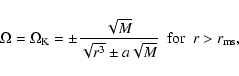
![\begin{displaymath}
\frac{\mathcal{R}}{E^{2}}=\left[(r^{2}+a^{2})-a\lambda\right...
...}}{E^{2}}+(\lambda-a)^{2}+r^{2}\frac{m^{2}}{E^{2}}\right]\cdot
\end{displaymath}](/articles/aa/full/2004/03/aah4692/img150.gif)
![\begin{displaymath}
\epsilon(r)\propto \exp\left[-\frac{R_{\rm t}}{r}\alpha\right] \ r^{-\beta},
\end{displaymath}](/articles/aa/full/2004/03/aah4692/img192.gif)
![\begin{displaymath}
\epsilon(r)\propto \exp\left[-\frac{(r-R_{\rm t})^{2}}{\sigma_{\rm r}^{2}}\right]\cdot
\end{displaymath}](/articles/aa/full/2004/03/aah4692/img195.gif)