A&A 413, 1045-1063 (2004)
DOI: 10.1051/0004-6361:20031582

Abundances of Na, Mg and Al in nearby metal-poor stars

T. Gehren¹ - Y. C. Liang^1,2 - J. R. Shi^1,2 - H. W. Zhang^1,2,3 - G. Zhao^1,2

1 - Institut für Astronomie und Astrophysik der Universität München, Scheinerstr. 1, 81679 München, Germany
2 - National Astronomical Observatories, Chinese Academy of Sciences, Beijing 100012, PR China
3 - Department of Astronomy, School of Physics, Peking University, Beijing 100871, PR China

Received 17 June 2003 / Accepted 7 October 2003

Abstract
To determine the population membership of nearby stars we explore abundance results obtained for the light neutron-rich elements ²³Na and ²⁷Al in a small sample of moderately metal-poor stars. Spectroscopic observations are limited to the solar neighbourhood so that gravities can be determined from H IPPARCOS parallaxes, and the results are confronted with those for a separate sample of more metal-poor typical halo stars. Following earlier investigations, the abundances of Na, Mg and Al have been derived from NLTE statistical equilibrium calculations used as input to line profile synthesis. Compared with LTE the abundances require systematic corrections, with typical values of +0.05 for [Mg/Fe], -0.1 for [Na/Fe] and +0.2 for [Al/Fe] in thick disk stars where [Fe/H] $\sim -0.6$. In more metal-poor halo stars these values reach +0.1, -0.4, and +0.5, respectively, differences that can no longer be ignored.

After careful selection of a clean subsample free from suspected or known binaries and peculiar stars, we find that [Na/Mg] and [Al/Mg], in combination with [Mg/Fe], space velocities and stellar evolutionary ages, make possible an individual discrimination between thick disk and halo stars. At present, this evidence is limited by the small number of stars analyzed. We identify a gap at [Al/Mg] $\sim -0.15$ and [Fe/H] $\sim -1.0$ that isolates stars of the thick disk from those in the halo. A similar separation occurs at [Na/Mg] $\sim -0.4$. We do not confirm the age gap between thin and thick disk found by Fuhrmann. Instead we find an age boundary between halo and thick disk stars, however, with an absolute value of 14 Gyr that must be considered as preliminary. While the stellar sample is by no means complete, the resulting abundances indicate the necessity to revise current models of chemical evolution and/or stellar nucleosynthesis to allow for an adequate production of neutron-rich species in early stellar generations.

Key words: line: formation - line: profiles - stars: fundamental parameters - stars: abundances - stars: late-type

1 Introduction

Traces of an early Galactic evolution can be found in the spectra of low-mass stars. Such stars are in a core hydrogen-burning stage which guarantees that chemical elements seen in their atmospheres are respresentative of the gas out of which they formed. Whenever the stellar parameters make possible the determination of stellar ages, the observed element abundances can put constraints on evolutionary time scales and the conditions under which stellar populations emerged. In particular the light metals Na, Mg, and Al are synthesized in nuclear burning stages that occur during the advanced evolution of massive stars. The extra neutrons in the ²³Na and ²⁷Al nuclei are a sign of the C- and Ne-burning processes that have been calculated under various assumptions (see Arnett 1996). Similar as the evolution of s- and r-process isotopes these nuclei may disclose information about the nature and the physical parameters of the first stellar generations, whether Population III or II.

Na, Mg and Al are in principle easy to observe in unevolved stars of spectral types F and G, because they have spectral lines of different strength and excitation in the visual wavelength region. Yet recent investigations of metal-poor stars have not converged toward a consistent picture (see Tomkin et al. 1985, 1992; Edvardsson et al. 1993; Timmes et al. 1995; McWilliam et al. 1995; Pilachowski et al. 1996; McWilliam 1997; Carretta et al. 2000; Chen et al. 2000; Fulbright 2000; Prochaska et al. 2000). Part of the problems connected with the interpretation of observed data seems to be owed to a large scatter of the resulting abundance ratios, and this can be due to a significant weakness in methodical approach, the assumption of local thermodynamic equilibrium (LTE) in the stellar atmospheres.

Large computers and even larger telescopes have made it relatively easy to obtain data for stars that could not be observed with high-resolution spectrographs only a decade ago. Since then most efforts have been focused on observing faint stars that are extremely metal-poor, mostly in hope to detect stars as near as possible to the oldest stellar population III. The results have opened a new empirical approach to the earliest Galactic nucleosynthesis, but they have not settled the basic questions: what type of stars were the first in the evolution of the Galaxy? What were the initial properties of the first stellar generations, and how did special elements and isotopes enter the chemical evolution of the Milky Way? Fuhrmann (1998, 2002) has repeatedly and almost convincingly argued that the local population of metal-poor dwarfs represents essentially the thick disk, and that halo stars constitute only an extremely tiny fraction of the local stellar mass which may or may not have been accreted from external star clusters or galaxies. Fuhrmann (2000) and Bernkopf et al. (2001) find that if there is any difference at all, the ages of both halo and thick disk stars must be very similar, i.e. beyond 12 Gyr. In fact, the identification and population membership of single stars has always remained somewhat arbitrary, in that kinematics or metal abundance or age alone never gave a conclusive answer. The most problematic identifier is the metal abundance because we learnt that there may exist low-abundance stars that kinematically would fit to thick disk velocities (Norris et al. 1985), and quite generally there may be a significant overlap of the populations in some, if not all, of the three parameters.

The status of the Galactic halo component is fairly uncertain. Its contribution to Galactic mass and its origin are far from being understood. Before following any more speculations it therefore seems worthwhile looking for further empirical signs of population membership. While metal abundance in general is admittedly a bad measure of the Galactic evolution time, metal abundance ratios could be used instead, if the origin of certain elements could be properly assigned to processes of nucleosynthesis and corresponding stellar masses and time scales. Consequently, it takes a longer evolutionary time to produce s-process elements than is necessary for r-process nucleosynthesis because the involved stellar masses are different. Equally, the production of $\alpha$-elements is followed on a shorter time scale than that of iron, again due to the stellar masses involved in supernovae of type II and Ia, respectively. The question arises: will there be a definite abundance ratio which allows the individual discrimination of a halo star from a thick disk star? There appears to be empirical evidence for [Eu/Mg] being such an element ratio that allows a well-defined distinction between [Eu/Mg] $\sim 0.0$ in stars of the disk populations (including the thick disk) and [Eu/Mg] $\sim 0.3$ in halo stars (Mashonkina et al. 2003). This is particularly interesting because both elements are thought to be produced in massive stars shortly before or during the SN II explosion. Since europium is hard to observe in metal-poor stars other elements might be preferred, and the abundances of ²³Na, ²⁴Mg and ²⁷Al could provide such a discriminator.

Our investigation starts with a definition of our stellar samples and the reason for a separation between the mildly metal-poor sample and the extremely metal-poor halo stars. In the following section we will also discuss the observations and the extraction of echelle spectra, followed in Sect. 3 by a short presentation of the stellar parameters, temperature and gravity, microturbulence and iron abundance and the methods involved. Section 4 explains the conditions and models for which spectral line synthesis was obtained. NLTE line formation will emerge as the most important factor of the analyses. It will become evident, how much NLTE and LTE abundance results differ. This section will also show the element abundance results including a discussion of the abundance ratios and their comparison with recent analyses of other groups. The kinematic properties of the stars are described together with a very preliminary determination of stellar ages in Sect. 5. Although we are still far from a sound interpretation in terms of Galactic evolution and population membership, the final section adds a number of interesting conclusions.

   
2 Observations and data reduction

2.1 The stellar samples

Our approach towards a representative abundance investigation is aimed at analyzing a limited sample of 162 high-proper motion stars (Carney & Latham 1987; Sandage & Fouts 1987) with sub-solar metal abundances indicated by broad-band colour excess $\delta (U-B)$. The stellar positions of the basic set of observations to be carried out at the 2.2 m telescope on top of Calar Alto are restricted towards declinations $\delta > -10\hbox{$^\circ$ }$. V magnitudes are selected to be brighter than 10.5 in order to permit a reasonable S/N ratio. Since our interest is focused on turnoff stars, we observe only stars with 0.35 < B-V < 0.72; and finally, the resulting absolute magnitudes based on H IPPARCOS observations are selected to lie between 3.0 and 5.5.

	Figure 1: Colour-magnitude diagram of 162 unevolved near-turnoff stars fulfilling the selection criteria, based on H IPPARCOS parallaxes. Filled circles refer to observed stars, open circles to the rest of the sample. Star-like symbols document the metal-poor comparison sample. Symbol sizes increase with the $\delta (U-B)$ excesses in the three intervals [0.10 ...0.14], [0.14 ...0.20] and >0.20.
Open with DEXTER

This sample contains but a very few extremely metal-poor stars. Thus we have extended our analysis to include as many metal-poor stars as possible that do not fit the above selection criteria. Spectra for these stars were taken from recent observations carried out mostly for different purposes. The results obtained for the second sample will serve as a control of the properties obtained for the less metal-poor stars of disk and halo components. The stellar samples are displayed in Fig. 1, which gives an account of the type of stars involved. The sample shown in Fig. 1 will not be complete in that it is not volume-limited. It is essentially flux-limited, with colour excess and availability of H IPPARCOS parallaxes providing the most important restrictions.

2.2 Spectroscopic observations

High-resolution spectra analyzed in our present investigation were obtained from two sources. Data for 38 moderately metal-poor stars were observed with the FOCES fiber optics echelle spectrograph fed by the 2.2 m telescope of the DSAZ at Calar Alto Observatory during August 2001, whereas spectra of 14 metal-poor halo stars were observed with the UVES echelle spectrograph mounted at the ESO VLT2 during March 2001. Throughout this paper the two samples will always be distinguished.

The FOCES observations of the stars in the northern hemisphere all cover a spectral range from 3700 to 9800 Å on a total of 97 spectral orders. The spectra were exposed on a 2048² CCD chip with $24~\mu$m pixel size, providing a spectral resolution of $R \sim 40~000$ per 2 pixel resolution element. Basic observational data are given in the upper part of Table 1. For nearly all stars the total exposure time was divided into 3 single exposures to allow redundant data extraction. Unfortunately, due to substantial extinction from sky haze and only medium seeing properties some of the exposures do not show the expected signal. Yet most of the combined spectra display a $S/N \sim 200$ near  ${\rm H}\alpha$. UVES observations cover a spectral range between 3300 and 6650 Å with gaps of $\sim$100 Å around 4570 Å due to the beam splitter and near 5580 Å at the edge of the butted CCD. The spectral resolution is around R = 60 000. These observations were originally intended to show a high signal in the blue (see Mashonkina et al. 2003). Consequently the green/red spectra have a S/N near 300 in most of the single exposures. Again, 3 exposures were taken for each of the stars, for which the data are found in the bottom section of Table 1.

Data extraction followed the standard automatic IDL program environment designed for the FOCES spectrograph (Pfeiffer et al. 1998), but with slight modifications also applicable to the UVES data. All echelle images including flatfield and ThAr were corrected for bias and scattered light background. Objects and ThAr exposures were extracted and corrected for flatfield response. Finally, bad pixels were detected and as far as possible removed by comparison of the 3 single exposures. This was particularly simple because most of the exposures were obtained in a time sequence. After wavelength calibration each of the spectra underwent a correlation with the solar spectrum to determine the radial velocity, before the single exposures were co-added without wavelength shift, thus ignoring any possible variations of radial velocity. This procedure could have been improved applying independent resampling of the single exposures before co-adding. However, it turned out that all velocity variations were well below a detectable level of 0.3 km s^-1, whereas the subsequent spectrum analyses did not give any sign of kinematically broadened absorption lines. Thus we preferred to trade the disadvantage of a small velocity error against the advantage of co-adding single spectra without resampling.

Table 1: Spectra obtained with the FOCES echelle spectrograph at the Calar Alto 2.2 m telescope in August 2001 (top section), and with the UVES echelle spectrograph at the ESO VLT telescope in March 2001 (bottom section). Columns are mostly self-explanatory. Parallaxes (mas), their errors $\sigma$, and proper motions (mas/y) are taken from the H IPPARCOS catalogue (ESA 1997). N and $t_{\rm exp}$ refer to the number of spectra taken and the total exposure time (s).

2.3 Notes on data reduction

	Figure 2: Sample spectra of the velocity-corrected SB2 stars including HD 99383. The two components have been marked for the Cr I 201 line at 5254.98 Å. The flux axis is on an arbitrary scale, compressed to show approximately the same dynamic range for each star. The solar flux spectrum of Kurucz et al. (1984) is shown for comparison.
Open with DEXTER

Table 1 shows that all of our stars belong to the solar environment, most of them traversing inside a sphere of 100 pc radius. The SB2 comments in the rightmost column refer to a simple inspection of the extracted spectra which leads to the detection of 6 double-lined binaries with well-resolved line pairs. Two of the stars are also found to have substantial emission in the Ca II H and K lines. We comment on these stars below. 6 Stars were subsequently found to be single-lined binaries by Latham et al. (2002), and one star, HD 99383, was reported by Nissen et al. (2002) as a double-lined binary, whereas our spectra do not indicate a second line system. Even without further statistics (see Latham et al. 2002) it is evident here that the local volume of high-proper motion stars contains a large fraction of binaries. Since the determination of stellar parameters from binary spectra requires much more observational effort, most of the stars marked as binaries in Table 1 have been removed from our sample. Out of 38+14 stars observed there will be analyses only for 27+11 stars with high enough signal, for which no conclusive spectral signs of binarity are found. The following notes for some of the stars give an account of known spectral peculiarities.

HD 133621, HD 134113: Orbital solutions by Latham et al. (2002) were recognized only after the observing runs.

HD 141335 (G224-81): Orbital solution by Goldberg et al. (2002) was recognized only after the observing runs. Spectrum is double-lined with the second component offset by $\sim$28 km s^-1 to the red (see Fig. 2). Mg I b lines show unusually strong wings with a clear asymmetry to the red.

HD 142267: Noted by Hünsch et al. (1999) as a weak X-ray emitter. Nidever et al. (2002) list it as a possible radial velocity variable, but with questionable evidence from only 2 observations. Ca II H+K seem to be slightly filled in, but the absorption line spectra are unconspicuous.

BD+68$^\circ$ 901: Core emission in the Ca II H+K lines (see Fig. 3). The spectrum looks normal.

	Figure 3: Relatively strong emission in the cores of the Ca II H+K lines is found in the (normalized) spectra of BD+68$^\circ$ 901 and HD 224930 (the flux of the latter is offset by -0.1).
Open with DEXTER

HD 173084: Known as visual binary star with separation of 0.36 arcsec. Double-lined spectrum with a velocity offset of ${\sim}{-}16$ km s^-1 (see Fig. 2).

HD 184855 (G92-15), HD 210631 (G18-35), G217-8, HD 10443 (G71-27): All four stars now have orbital solutions published by Latham et al. (2002).

G261-10: Double-lined spectroscopic binary with second component shifted towards ${\sim}{-}17$ km s^-1 (see Fig. 2). This star is on the list of Latham et al. (2002), but with no indication of RV variation.

HD 198300 (G230-49): Noted by Smith & Churchill (1998) because of faint Ca II H+K emission, which is not well documented on our spectra.

HD 200580: Only recently identified as a visual binary using speckle interferometry (Mason et al. 2001). The angular distance of the two stellar components is only 0.13 arcsec.

HD 221950: Cited by Clausen et al. (1997) as a photometric primary star, the spectrum shows a clear double-lined structure with velocity separation of ${\sim}{-}71$ km s^-1 and components of similar strength. Ca II H+K display a filled-in core with significant asymmetry. As seen in Fig. 2, the lines of both components are significantly broader than typical line widths of other stars observed with the same instrument settings. Explained by rotation alone, the additional line widths would fit to $V\sin i \sim 11.5$ km s^-1.

HD 224930: Spectroscopic binary (Underhill 1963), secondary component is approximately 3 mag fainter. Ca II H+K lines with core emission (see Fig. 3).

HD 29907: Single-lined spectroscopic binary (Lindgren & Ardeberg 1996).

CD-52$^\circ$ 2174: Double-lined spectroscopic binary with second component shifted by ${\sim}{-}13$ km s^-1 (see Fig. 2).

BD-3$^\circ$ 2525: Clearly double-lined spectroscopic binary with ${\sim}{-}17$ km s^-1 separation. Greenstein & Saha (1986) have published an orbit for a single-lined binary. Latham et al. (1988) revised the binary orbit and reported the double-lined structure of the spectra (see Fig. 2).

HD 99383: Nissen et al. (2002) list this star as a double-lined spectroscopic binary. As indicated in Fig. 2, there is no second line system found in our spectra.

Of all known binary stars only HD 200580, HD 224930, and HD 29907 have been retained for spectroscopic analysis, and we will pay special attention to the abundance results of these stars. The other spectroscopic binaries will be analyzed separately. The second line system in double-lined binary spectra is not always detected very easily. Using a correlation analysis with reference to the solar flux spectrum of Kurucz et al. (1984) the spectral binary structure becomes more evident. A small part of the SB2 spectra is displayed in Fig. 2, where the two components have been marked for the Cr I 201 line near 5255 Å. Note that the spectrum of HD 99383 is clearly single-lined in our exposures. However, the lines appear slightly broader than those of CD-52$^\circ$2174 or BD-3$^\circ$2525.

The existence of stellar chromospheres has been confirmed for solar-type members of the thin disk, but also for metal-poor subdwarfs (Smith & Churchill 1998). Our blue spectra seem to show chromospheric H+K line reversals for many of the stars analyzed here, all of them with B-V < 0.75. Although the relatively low signal does not allow to confirm this for individual stars, it is seen more clearly in the mean spectra of both samples.

   
3 Atmospheric models and stellar parameters

Stellar atmospheric models have been calculated for the individual stars using plane-parallel one-dimensional stratifications of temperature and pressure. Our constraint of convective equilibrium is based on the mixing-length approach with a mixing-length parameter $\ell/H_{\rm p} = 0.5$ (Fuhrmann et al. 1993). Since the spectrum analysis is carried out differentially with respect to the Sun, the solar reference data are based on the same type of atmospheric model. Although a differential analysis does not rule out systematic errors - in particular, when large differences in basic parameters are encountered - this way of comparing abundances for a large sample of stars seems to us more adequate than the use of so-called absolute oscillator strengths.

Plane-parallel atmospheres are very unspecific in modeling kinematic properties of the emitting gas flows. This is immediately evident from the solar granulation, and the unsatisfactory situation must be improved with the introduction of the microturbulence velocity. The concept of micro- and macroturbulence is far from hydrodynamic reality but surprisingly successful in describing the total integrated flux blocked by an absorption line, and also the overall profile shape of the emerging line flux. However, it is limited to symmetric profiles. The present status of horizontally homogeneous atmospheres is also limited by the application of local thermodynamic equilibrium (LTE). This introduces an inconsistency between the atmospheric structure and the formation of absorption lines, which is not too important in stars near the main sequence, but it may become more influential in slightly evolved stars of reduced metal abundance. Except for these considerations our models include the physics that provide the transport of energy using essentially 5 free parameters to fit the observed line spectra. These are: effective temperature $T_{\rm eff}$, surface gravity $\log g$, microturbulence velocity $\xi_{\rm t}$, metal abundance [Fe/H], and $\alpha$-element abundance ratio [$\alpha$/Fe], where the last 3 parameters enter the opacity distribution functions (ODF), which determine the optical depths. We use the ODF data provided by Kurucz (1992), but rescaled by $\Delta\rm [Fe/H] = -0.16$ to account for a meteoritic iron abundance $\log\varepsilon_{\rm Fe,\odot} = 7.51$ (Anders & Grevesse 1989). Transfer and constraint equations are fully linearized with respect to temperature and pressure. Our use of ODFs is restricted to the calculation of the model atmosphere. The NLTE formation of absorption lines instead uses a full opacity sampling (see Sect. 4).

Table 2: Metal lines used to determine element abundances. f values and damping constants have been determined from solar spectrum fits.

The most important problem is therefore the determination of the basic stellar parameters. Both $T_{\rm eff}$ and $\log g$ have a strong influence on the final abundances. Effective temperatures are derived from fitting the wings of the Balmer line profiles ${\rm H}\alpha$ and ${\rm H}\beta$ (Fuhrmann et al. 1993, 1994). We do not apply the broadening theory recently published by Barklem et al. (2000), because it does not reproduce the temperature of the Sun, which would have spoiled the differential nature of our investigation. Instead we use the resonance broadening as described by Ali & Griem (1965, 1966). Our results are in reasonable agreement with data obtained using the Infrared Flux Method (Alonso et al. 1995, 1996). The difference between our temperature scale and that obtained with the IFM for 7 stars in common between 5000 and 6200 K is $\Delta T_{\rm eff}= +40 \pm 78$ K. As mentioned in the introduction, all stars in our sample have trigonometric parallaxes observed with H IPPARCOS (1997). Therefore we evaluate the surface gravities $\log g$ with the help of $[g] = [{M/L}]+4[T_{\rm eff}]$, where the square brackets have a similar meaning as in the definition of [Fe/H]. While the stellar luminosities require the knowledge of the visual magnitude, the interstellar extinction (which is negligible for most of our stars), the bolometric correction (BC) as tabulated by Alonso et al. (1995), and the parallax, the resulting value of $\log g$ depends also on the stellar mass. The masses have been estimated from the evolutionary tracks of the $\alpha$-enhanced stellar models calculated by VandenBerg et al. (2000), with interpolation of abundances (see also Sect. 5.2). The resulting values for BC, $M_{\rm bol}$, and $M/M_\odot$ are given in Table 3. Apart from systematic shifts in the theoretical $M_{\rm V}$ vs. $\log T_{\rm eff}$ diagram, the mass uncertainty introduced by effective temperature errors is between 0.02 and 0.05 $M_\odot$. This transforms into a relatively small error of $\sigma(\log g) < 0.03$, to which the parallax error has not yet been added. The final error of the surface gravity then will be around 0.05 for most of the stars.

Two other stellar parameters, the "metal'' abundance [Fe/H] and the microturbulence $\xi_{\rm t}$, are evaluated in close interaction. For this purpose a list of selected Fe II lines is used to synthesize line profiles for given $T_{\rm eff}$ and $\log g$. These lines are found, together with the line data determined from the solar spectrum, at the end of Table 2. We mention here that Fe II lines are synthesized under the assumption of LTE. The choice of the line list follows the requirement of minimum blends and the need to detect them (or at least a subset thereof) in extremely metal-poor stars. These lines have been used in a closed loop iteration to determine [Fe/H] with minimum scatter for a given $\xi_{\rm t}$. The final internal accuracy of the metal abundance is around $\sigma$([Fe/H]) $\sim 0.05$ and $\sigma(\xi_{\rm t}) \sim 0.1$ km s^-1.

Stellar atmospheres on the subgiant branch or near the bottom of the giant branch depend on the specification of another abundance parameter, [$\alpha$/Fe], which determines a significant fraction of the free electron pool at cooler surface temperatures. [$\alpha$/Fe] is dominated by all $\alpha$ elements with a low enough ionization energy (which excludes oxygen and neon). This requires the knowledge of abundance ratios, of which [Mg/Fe] is determined by NLTE analyses, whereas [Si/Fe] or [Ca/Fe] were estimated assuming values lower than for [Mg/Fe]. Fortunately, the determination of [$\alpha$/Fe] is not crucial for our analysis since none of the stars in Table 3 is in the critical range of temperatures and gravities. Therefore, all our atmospheric models are calculated assuming [$\alpha$/Fe] = [Mg/Fe]. The final atmospheric model parameters are iterated whenever [Mg/Fe] or $\xi_{\rm t}$ deviate from the initial determination during the subsequent abundance analysis.

	Figure 4: Typical example of collision-dominated Na I population departure coefficients $b_n = N_n^{\rm NLTE}/N_n^{\rm LTE}$ in the moderately metal-poor star HD 148816. The kinetic equilibrium calculations are described in the text.
Open with DEXTER

  
4 NLTE line formation

Deviations from local thermodynamic equilibrium (LTE) in stars are generally expected in gaseous stratifications in which the kinetic equilibrium is determined by non-local interaction processes such as radiation transfer. Since collisions always act as sources of thermalization, the dominance of radiative processes is to be measured against collisional interactions. Typically, in hot stars the radiation field outperforms electronic collisions by an order of magnitude, whereas in cool stellar atmospheres the radiation field is much weaker, and collisions play a more important role. Therefore it is by no means evident why stars with atmospheres as cool as the Sun should be affected by NLTE conditions. However, as explored by Baumüller et al. (1997, 1998) and Zhao et al. (1998, 2000), two reasons for deviations from LTE are found in the atmospheres of metal-poor FG-type stars even near the main sequence. The collision rates are reduced due to a decrease of the electron density with metal abundance, because a large fraction of the electron donors at temperatures below 7000 K consists of metals instead of hydrogen. The radiation field is absorbed by a smaller fraction of metal atoms and ions (predominantly in the near UV), and as a result the photoionization rates tend to increase with falling metal abundance. Both effects are particularly important in such stars for ions far from their ionization maximum, such as most of the neutral metals with ionization energies below 8 eV. These elements are more than 90% ionized, and the neutral atoms become a minority that is sensitively reacting on particle interactions. On the other hand, the kinetic equilibrium of majority ions as Ca II or Ba II is often balanced by line transitions (see Mashonkina et al. 1999).

While collisions between atoms and electrons or heavier particles seem to be very similar for the different atomic species, photoionization rates not only depend on the radiation field (and the line blocking), but at least as much on the atomic properties. Whereas atoms such as Na I have very small photoabsorption cross-sections and hence photoionization rates, the situation is completely different for atoms of Mg I, Al I, and even Fe I. Their atomic structure provides them with particularly strong photoabsorption cross-sections, and their photoionization rates can be very large.

Table 3: Final stellar parameters and abundances of the program stars. For the description of stellar masses and ages see Sect. 5.

Quite generally, in cool metal-poor stellar atmospheres, atoms of the first kind cascade recombining electrons down to their ground state because there is no efficient ionization. Simultaneously, the reduced electronic collisions cannot maintain a thermal excitation equilibrium. Displayed in Fig. 4, the level populations of this type of atom are above those of thermal equilibrium in the region of line formation associated with that level. Consequently, the increased opacities in the line cores and inner wings produce a line optical depth scale that is significantly shifted to the outer layers, and the line source functions are larger than the Planck function. Both effects work in opposite directions, but the result is dominated by the increased optical depth scale, and the Na I D lines are intrinsically deeper in NLTE calculations than in LTE. Therefore a reduced NLTE element abundance is necessary to fit an observed line profile.

Although sodium is not the only example for such a downward cascade in a neutral metal, the opposite case of enhanced photoabsorption cross-sections seems to be more common. Examples for photoionization-dominated neutral metals have been given above. At present, these atomic species present a considerable challenge to the theory of atomic interactions and their kinetic equilibrium. The reason for that is evident in the solar spectrum, where the strongest absorption edges in the near UV are not produced by the hydrogen atom despite of its extremely high abundance. It is the Al I ground state with its low ionization energy of only 5.98 eV that produces the deepest cut in the solar flux at 2070 Å, followed by the Mg I $3\rm p^3$P$^{\rm o}$ ionization edge at 2510 Å. While the other low-excitation levels of Mg I, $\rm 3s^1$S and $\rm 3p^1$P$^{\rm o}$ have also strong photoabsorption cross-sections, all other bf opacity sources in the near UV are less important. Fe I is, however, a notable exception. According to Bautista's (1997) calculations its large number of low-excitation levels each has a photoabsorption cross-section significantly in excess of what is found in more simple atomic configurations. Here, the high number of large photoionization rates up to levels of 4 or 5 eV excitation energy produces an important sink to the population of neutral iron. A typical example of photoionization-dominated departure coefficients is given in Fig. 5.

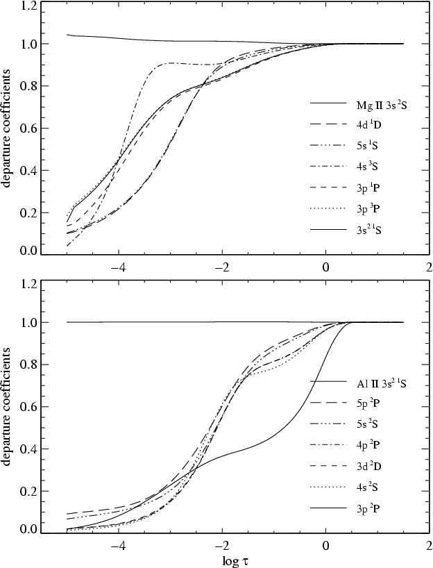	Figure 5: Typical example of photoionization-dominated Mg I departure coefficients in the moderately metal-poor disk star HD 157089 (top) and the Al I departure coefficients in G69-8 (bottom). In spite of hydrogen collisions all neutral energy levels are strongly underpopulated.
Open with DEXTER

The strength of these absorption edges gives rise to different degrees of depopulation of neutral metal levels. In terms of statistical equilibrium this is due to the inefficiency of both electronic ionization and excitation to compensate for the large photoionization rates whenever simple calculations as those of van Regemorter (1962) or Seaton (1962) are employed. To avoid an unrealistic excitation/ionization balance - this can be controlled by comparison of line formation results for different absorbing levels and ionization stages - an additional source of thermalizing interactions is often included: collisions by neutral hydrogen atoms. For lack of any other theory, hydrogen collisions are treated in a very simple way. Originally it was proposed by Drawin (1968, 1969) for optically allowed transitions in rare gases. It essentially includes the dependence on excitation energy and transition probability, with all other possible effects integrated into a scaling factor $S_{\!\!\rm H}$. The scaling factor is intended to represent the whole ion, and it can only be determined empirically. Large scaling factors drive the excitation equilibrium towards thermal conditions (LTE) whereas small factors produce the largest NLTE effects. It is the determination of this factor which is most discussed in the literature, and there have been proposed deviations from the simple constant multiplication factor such as excitation-dependent scaling (Zhao et al. 1998). A few general results have emerged,

• Empirical evidence beyond any doubt requires the existence of some additional source of thermalization in cool metal-poor stars, where electron donators such as iron, magnesium, silicon or even sodium are significantly underabundant.
• Although it is only an order-of-magnitude approximation we regard the representation of electron collisions in van Regemorter's formula as more reliable than any other type of theory for thermalization interaction, so the existence of hydrogen collisions is the single acceptable solution to compensate large radiative rates.
• The existence of photospheric Rydberg transitions of Mg I and Al I in the infrared solar spectrum implies that hydrogen collisions must be inefficient at highly excited levels in order to allow for population inversion.
• Since hydrogen collisions are needed to compensate for the large photoionization rates - in particular of near-ground state levels, their strength must be determined in reaction to the strength of the photoionization rates and cannot be set to zero.

In particular in photoionization-dominated atoms the compensation between radiative and collisional processes can be judged by determining the dependence of element abundances that fit the observed profiles of lines with increasing excitation energy. Both in LTE and with badly chosen hydrogen collision scaling factors in NLTE the line spectra will not result in a common abundance but display a sometimes strongly excitation-dependent behaviour. This is different from the dependence in case of a wrong temperature because it does not necessarily depend monotonously on excitation energy. However, the empirical choice of $S_{\!\!\rm H}$ requires the separate (and thus iterative) determination of microturbulence.

4.1 Atomic models

Our present investigation is based on the atomic properties documented in a number of earlier reports (Baumüller et al. 1996, 1997, 1998; Zhao et al. 1998, 2000), where most of the problems have been described in more detail. It deviates from these results in that our atomic models have been redesigned. The number of levels was extended to include all known terms plus some hydrogenic terms near the ionization edge. All bf radiative cross-sections have been included from close-coupling calculations of Butler (1993) and Butler et al. (1993). At the same time the opacity distribution function background has been replaced by an opacity sampling method. The reason for this change lies in the extremely strong UV blocking factors introduced by the ODF method, which do not fit to the observed solar spectrum. The change from ODF to OS background opacities was also performed to remove the corresponding background opacity dependence on the NLTE elements themselves. Therefore, compared with earlier published data, the new models produced slightly different population departure coefficients, which in turn required a new empirical determination of the hydrogen collision factors $S_{\!\!\rm H}$. The full analysis of all observed spectra including the solar spectrum of Kurucz et al. (1984) allows the choice of a reasonable compromise which, iterated together with all basic stellar parameters, led to the values of $S_{\!\!\rm H}= 0.05$ for Mg I and Na I, whereas Al I required a smaller value of $S_{\!\!\rm H}= 0.002$. These numbers differ from those used before because the photoionization rates were considerably enhanced with reduced OS background opacities. There is also no longer an advantage in assuming an excitation-dependent collision factor as in Baumüller et al. (1996) or Zhao et al. (1998). Stronger thermalization would not fit to a common mean abundance scale including all lines analyzed here (see below). In particular, LTE abundances always produce significant differences between resonance or low-excitation and subordinate lines of all three elements.

All calculations have been carried out with a revised version of the DETAIL program (Butler & Giddings 1985) using accelerated lambda iteration following the extremely efficient method described by Rybicki & Hummer (1991, 1992). As described in Sect. 3, the analyses for all stars were iterated until basic stellar parameters and single line NLTE abundances were consistent. In spite of substantial changes in the atomic models, the basic properties of the Na, Mg and Al abundances are still the same as in our previous analyses.

   
4.2 Spectrum synthesis

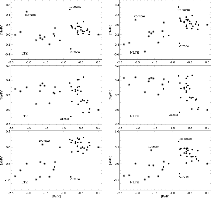	Figure 6: Abundance ratios [X/Fe] for both LTE (left) and NLTE (right) analyses. Filled circles refer to our moderately metal-poor sample, star-like symbols to the extremely metal-poor comparison stars. Some apparently peculiar stars are marked (see text). Differences between LTE and NLTE abundance ratios are displayed in Fig. 12.
Open with DEXTER

Our analysis rests on between 6 and 8 lines for each of the elements considered. Since our results are based on a differential analysis with respect to the Sun, Table 2 lists the relevant line data with their final solar fit values. The Fe II lines have been synthesized under LTE conditions only, because they are not affected by NLTE departures. For Na I, Mg I and Al I, profile synthesis has been performed for both LTE and NLTE, however, the data in Table 2 refer only to the NLTE analysis. Our fit to the solar line spectrum requires some priority as far as the line data are concerned. Thus the primary choice of input data are the oscillator strengths, while the damping constants have been adjusted to fit the line wings. The resulting values of the van der Waals damping constants are mostly near to those calculated according to Anstee & O'Mara's (1991, 1995) tables, though they are systematically lower by 0.1 to 0.3 dex. This is similar to the damping constant fits for neutral iron lines (Gehren et al. 2001). We note here that, accepting Anstee & O'Mara's damping constants without change, some of the oscillator strengths would have to be modified substantially in order to produce a solar line profile fit.

Doppler broadening of the line profiles follows the usual assumption of random atmospheric motions represented by microturbulent velocities. Clearly, this representation by a single parameter, $\xi_{\rm t}$, is at its limit when high-resolution spectra are analyzed. There can be no doubt that lines of the Fe II multiplet 42 are formed under conditions quite different from those of the other multiplets. Similar problems are found among the lines of the other elements. As a result, we have fitted the observed metal line profiles with a maximum of accuracy, however, being aware that there remains an uncertainty in the profile shapes that is equivalent to some 0.05 dex in abundance results. In fact, this may be the limiting accuracy obtainable in a plane-parallel atmospheric model. We note that this uncertainty is significantly smaller than most of the NLTE effects found in the metal-poor stars.

Spectrum synthesis is performed interactively using the IDL/Fortran-based SIU software package of Reetz (1993). It was designed to use large databases including relevant data for ion and molecular lines. Once that model atmosphere and NLTE calculations are available, all spectrum synthesis calculations, whether LTE or NLTE, are performed in real time and displayed on the screen for further evaluation. All parameters can be adjusted, which is particularly important for the external broadening of line profiles encountered by macroturbulence, rotation, or the spectrograph entrance slit. Interactive spectrum synthesis with SIU allows for a full consideration of profile blends, hyperfine structure and isotopic splitting, where abundances for each element can be adjusted individually. Consequently, all abundance results presented here are derived from profile fits using level populations, either calculated from Saha/Boltzmann distributions or from NLTE. For most of the lines in metal-poor stars, profile fits can be established with a simple Gaussian external broadening function.

4.3 Element abundances

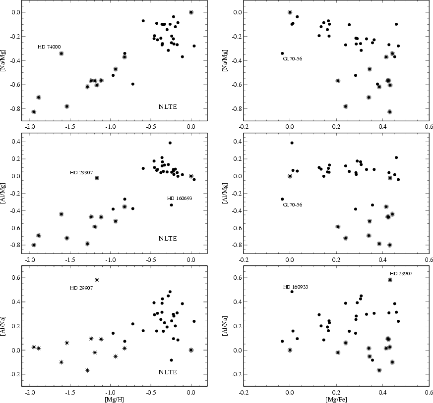	Figure 7: Abundance ratios [X/Y] for NLTE analyses as a function of [Mg/H] (left) and of [Mg/Fe] (right). Symbols are the same as in Fig. 6.
Open with DEXTER

Profile synthesis calculations were applied to all stars listed in Table 3. Line data were provided from solar profile fits, where LTE and NLTE cases were treated separately. With the exception of G242-4, for which the blue spectrum was of poor quality, this table presents both LTE and NLTE abundances averaged over all available lines. For most stars single line abundance errors are significantly reduced whenever NLTE calculations are involved. The final abundance scatter of single lines is between 0.02 and 0.09 for [Mg/Fe] in individual stars with a mean value of $\langle\sigma$[Mg/Fe] $\rangle = 0.040 \pm 0.017$ for all stars. For [Na/Fe] the corresponding values lie between 0.01 and 0.06 with $\langle\sigma$[Na/Fe] $\rangle = 0.026 \pm 0.014$ for all stars, and the data for [Al/Fe] are between 0.01 and 0.11, with $\langle\sigma$[Al/Fe] $\rangle = 0.039 \pm 0.035$. The highest abundance scatter is seen in the Mg and Al lines of HD 200580, for which the visual binary status seems to guarantee a composite spectrum. For that star the apparent mean abundances are enhanced, with [Na/Fe] = $0.36 \pm 0.03$, $\rm [Mg/Fe] = 0.46 \pm 0.08$, and [Al/Fe] = $0.67 \pm 0.10$.

No dependence of abundances on excitation energy is observed for the individual stars, because the final NLTE collision factors $S_{\!\!\rm H}$ have been optimized to avoid this. Although this is no guarantee for consistency of the abundance analysis, it is significantly better than if LTE were assumed. The basic results for LTE and NLTE are displayed in Fig. 6 demonstrating the enormous differences between LTE and NLTE line profile fit abundances.

Clearly, these differences are minor when [Mg/Fe] is concerned, with a limiting adjustment of ${\sim}{+}0.1$ dex for the extremely metal-deficient stars. Thus the overall run of [Mg/Fe] abundance ratios is changed only gradually. This is completely different for [Na/Fe] and [Al/Fe]. NLTE corrections for Na I increase from $\Delta\log\varepsilon_{\rm Na,NLTE-LTE} \sim 0.0$ at moderate metal deficiencies in the old thin disk to -0.4 in the extremely metal-poor stars. This confirms the results of Baumüller et al. (1998) obtained with slightly different atomic data and spectroscopic observations. By nature of the atomic interaction processes, the NLTE corrections for Na are largest for the resonance line doublet, which is the only spectral feature identified in the extremely metal-poor subdwarfs. The NLTE corrections for Al I are even stronger ranging from $\Delta\log\varepsilon_{\rm Al,NLTE-LTE} = +0.2$ for near-solar metal abundances to +0.5 in the extremely metal-poor subset which, formulated in the traditional chemical evolution picture, would transform Al from a straight "secondary'' element to a near "primary'' one.

Figure 6 may be used to identify stars that are not following the general abundance trends. As can be recognized from the comments in Sect. 2, such stars are no longer a minority in the whole stellar sample. The removal from spectral abundance analysis of roughly a third of the original star list due to binarity highlights the problems that are encountered. The remaining star list (Table 3) still includes the visual or single-lined binaries HD 29907, HD 200580, and HD 224930. It also includes metal-poor stars that do not give immediate evidence for a binary system but show X-ray emission (HD 142267) or emission cores in the Ca II H+K lines (BD+68$^\circ$ 901 and, again, HD 224930). Moreover, it includes a peculiar halo star, HD 74000, well known for its extreme nitrogen overabundance (Carbon et al. 1987) and its peculiar [Ba/Fe] and [Eu/Fe] ratios (Mashonkina et al. 2003), which together indicate that this star is probably not representative of a standard evolutionary scenario. Some of these stars, in particular HD 29907, HD 74000 and HD 200580, are immediately identified in Fig. 6. Each of them carries an extreme [Na/Fe] and/or [Al/Fe] ratio with no peculiarity found in [Mg/Fe]. G170-56 is a different case. Radial velocity variations of this star are not confirmed in Latham et al.'s (2002) list of observations (their Table 2), where any possible variation (<1 km s^-1 over a baseline of 15 yr) is hidden in the measurement error. With a quite unusual solar Mg/Fe ratio, both Na and Al are extremely underabundant.

4.4 Comparison with other analyses

Most of the analyses of other groups found in the literature are based on the assumption that LTE is a sufficient approximation of the thermodynamic state of the stellar atmospheres.

Cowan et al. (2002) reanalyzed a typical halo giant, BD+17$^\circ$ 3248, with an overall metal deficiency of $\rm [Fe/H] = -2.09$. They note a discrepancy when fitting the Na I D lines and the excited doublets at 5685 and 8190 Å which is typical for LTE results, as is their strong underabundance of Al derived from the resonance lines. The latter is found already in the work of Ryan et al. (1996), who admit that their values may be affected by departures from LTE.

Fulbright (2000, 2002), in his PhD thesis, analyzed a large number of metal-poor stars, of which 15 stars are in common with our present sample. His temperature scale differs from ours by $\Delta T_{\rm eff}= -177 \pm 104$ K, with a systematic trend running from -65 K for stars with near-solar metal abundance to -410 K for the extremely metal-poor star BD-4$^\circ$ 3208. Part of this large difference may be due to his use of overshooting model atmospheres which tend to produce an enhanced temperature stratification. The adjustment of effective temperatures until Fe I lines of different excitation energies fit to a common abundance value, is unsuitable to determine $T_{\rm eff}$. It is similar to the assumption of an LTE Fe II/Fe I ionization equilibrium to determine $\log g$. Therefore, his abundances of neutral ions, such as Na I and Al I should come out at values that are lower than ours. However, various approximations or assumptions interfere, and his abundance trends for ²³Na and ²⁷Al are buried in a scatter that our results do not reproduce. His sample may contain much more binaries or peculiar stars than ours, and his line data - collected from different sources - are responsible for at least some of the scatter.

Chen et al. (2000) published abundance data for a large sample of old (thin) disk stars with an admixture of thick disk members. Since their metal abundances are mostly well above [Fe/H] = -1, their [Na/Fe] ratios are only marginally affected by NLTE effects. They were aware of that [Al/Fe] is slightly more affected by deviations from LTE, even at thin disk metal abundances. In their Al/Fe ratios, calculated as all the other abundances under the assumption of LTE, the NLTE abundance corrections of ${\sim}{+}0.2$ are missing.

Thick disk stellar abundances have been investigated by Prochaska et al. (2000). They present results for a preliminary subsample of 10 stars with [Fe/H] between -0.43 and -1.09. Their admittedly small sample seems to present a similar gap in [Fe/H] between -0.7 and -1.0, slightly broader than seen in our data in Fig. 6. Their Na/Mg and Al/Mg ratios are derived under the assumption of LTE using only the subordinate lines of these elements (which are also part of our line list). The stars in their list all show a high [Al/Fe] ratio of $\sim$0.4, which is very similar to our data for thick disk stars derived under NLTE conditions. The [Na/Fe] data are around 0.1, also similar to our thick disk results under NLTE. The striking similarity can be understood, since both Na and Al results for excited lines differ only by a small amount (-0.1 or +0.1) between LTE and NLTE (see Fig. 12). The analysis is thus approximately on the same scale as ours, but includes only the thick disk.

Following Baumüller et al. (1998), Carretta et al. (2000; see also Gratton et al. 1999) seem to be the only group that applied NLTE calculations to sodium. Their results are very much in agreement with ours in that their NLTE corrections lead to a small metallicity-dependent increase of the [Na/Fe] ratios. Their scatter for medium-to-extreme metal-deficiency is, however, roughly two times the one we find. In view of the small sample we have analyzed here, it is not obvious whether that difference is significant.

   
5 Kinematic properties and stellar ages

Table 4: Kinematic data of the program stars. Velocities are in km s^-1. Radial velocities are own measurements, except for binaries. LSR velocities are calculated for a solar motion of $(U,V,W)_\odot$ = (10.0, 5.2, 7.2) km s^-1. Preliminary population membership assignments in the rightmost column are for thin disk (D), thick disk (T) and halo (H). See last section for an explanation.

In the last sections we have repeatedly referred to the population membership of single stars without specifying how we discriminate between different populations. We are of course fully aware of that such a discussion requires more than the interpretation of abundance ratios alone.

5.1 Galactic space velocities

Following the work of Roman (1950), the original classification of stellar populations was based much more on kinematics than on anything else. It is therefore of high priority to check if kinematic properties and abundance ratios have more in common than a coarse change of mean metal abundance itself. Although it was a general belief that metal-poor stars belong to the halo, and metal-rich stars to the disk, represented by populations II and I, respectively, the detection of the thick disk by Gilmore & Reid (1983) changed the simple picture of a spherical and a highly flattened stellar subsystem completely. Fuhrmann (2002) argues that in fact halo stars may constitute an extremely small minority of all Galactic stars, where most of the stars with intermediate kinematics instead belong to the thick disk.

The determination of Galactic kinematics, which are represented in the (U,V,W) system with respect to the Local Standard of Rest (LSR), is therefore an important aspect. In reference to the LSR we have adopted a solar motion of $(U,V,W)_\odot = (10.0,~5.2,~7.2)$ km s^-1 (see Binney & Merrifield 1998). For all stars except the known binaries we have entered our own radial velocity measurements, combined with H IPPARCOS parallaxes and proper motions. Table 4 provides the resulting space velocities including the total velocities calculated with reference to the LSR. The last column comments the population membership in a preliminary way which is based on a combination of kinematic properties, stellar ages and metal abundance ratios (predominantly [Al/Mg]) described in the discussion. For a number of stars the results are highly uncertain, and we will come back to these below.

The first inspection of the table shows that quite a number of stars in the sample seem to have kinematic properties that are far from the expected standard of any population. This is seldom a problem with a discrimination between thin and thick disk, because in particular the thin disk W velocities tend to be significantly smaller than those of the other populations. However, the most important discrimination between thick disk and halo cannot exclusively be based on the W velocity component. There are stars like HD 29907 with extreme high-velocity kinematics and very low metal abundance. However, the extreme velocity consists mostly of a radial component, the W velocity could even fit a thin disk star, and the metal deficiency is not extended to Al. Other stars such as HD 148816 or G170-56 even have retrograde Galactic orbits, but their metal abundance is near [Fe/H] = -0.8, their [Al/Mg] and [Na/Mg] ratios are far from typical for halo stars, and the [Mg/Fe] ratio of G170-56 is that of a typical solar-type thin disk star. HD 97320, in spite of its relatively low metal abundance of [Fe/H] = -1.24 and its [Mg/Fe] ratio of 0.41, kinematically fits more to thin disk properties. Thus, the remaining typical members of the halo population, originally included in our high-proper motion sample, are G188-22 and G242-4 (for which we unfortunately failed to determine the Al abundance). Most kinematic stellar properties are only loosely correlated with population membership. This holds at least for the U and W components, and for the $V_{\rm LSR}$ velocity. All these space velocities do not discriminate between thick disk and halo. The correlation between low V velocities and low [Al/Mg] ratios, however, is slightly more instructive.

The kinematic status of our sample is shown in the Toomre diagram presented in Fig. 8. Whereas we already learn from Fuhrmann's (1998) work that thin and thick disk are not easily identified kinematically, this seems to hold even more for the kinematic differences between thick disk and halo, in particular, since some stars may not belong to any of these populations. Stars like G170-56 or HD 29907 seem to have followed some peculiar history and may have been accreted from dwarf galaxies or star clusters. Yet, even comparing kinematics and abundance ratios alone, Fig. 9 suggests that the difference between thick disk and halo is relatively well described by the [Al/Mg] ratio and, less accurately, by the [Na/Mg] ratio. In both diagrams, the thin disk is separated in the upper right edge. The difference between thick disk and halo could be marked by a horizontal line corresponding to roughly [Al/Mg] = -0.15, and [Na/Mg] = -0.4. Together with special kinematical properties such as the V velocity component, the subdivision of the latter two components is already quite convincing.

	Figure 8: Toomre diagram of space velocities. Symbols are the same as in Fig. 6. As compared with our results, the diagram does not seem to offer a very good discrimination between populations.
Open with DEXTER

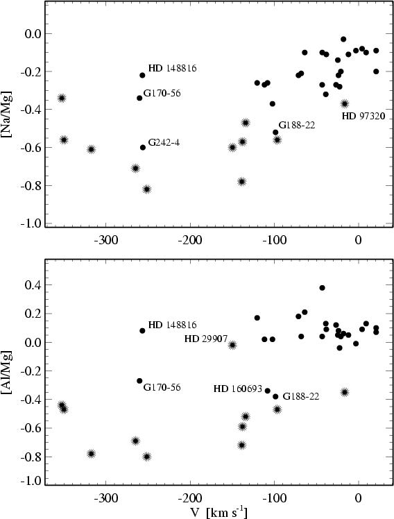	Figure 9: Correlation between abundance ratios and orbital V velocity component. Symbols are the same as in Fig. 6.
Open with DEXTER

   
5.2 Stellar ages

Another step towards the identification of single star population membership could be the age. Using the well-defined spectroscopic stellar effective temperatures together with the absolute magnitudes based on H IPPARCOS parallaxes (see Table 3) masses and approximate ages can be interpolated according to [Fe/H] and [$\alpha$/Fe] from adequate tracks of stellar evolution. Such calculations have recently become available through the work of VandenBerg et al. (2000), who updated and extended earlier work including new physics for the equation of state and opacities. There is no account for helium or metal diffusion at this time, but our most interesting objects may still be represented quite well differentially.

Using $T_{\rm eff}$ as coordinate of the HR diagram, there remains no need to introduce any empirical calibration to a colour index like B-V. Errors for most of the absolute magnitudes are small (exceptions are easily identified in Table 1). A typical result in Fig. 10 reproduces the interpolated stellar evolutionary track of HD 148816. The interpolation procedure is by no means simple, because changes between effective temperatures and ages for tracks of same composition but different masses are highly non-linear. Bergbusch & VandenBerg (1992) and VandenBerg et al. (2000) have proposed a suitable method that uses special morphological points, between which neighbouring evolutionary tracks may be safely interpolated. A similar approach was used here, so the interpolated final tracks always used $2\times 2\times 2$ tracks representing pairs of $M/M_\odot$, [Fe/H], and [$\alpha$/Fe], respectively.

We note that the knowledge of [$\alpha$/Fe] is as important as that of the other stellar parameters. Table 5 gives an account of the error propagation of the observed stellar parameters from which the unreliability of absolute stellar ages is immediately evident. Therefore we will only discuss comparative ages within the sample, where we have to remember that some of our parameters may in fact lead to uncertainties of the range indicated in the table. Compared with this the errors due to the interpolation method may be negligible.

Table 5: Error propagation of basic stellar parameters when interpolating tracks of stellar evolution for HD 148816. Variations are given with respect to the final parameters in Table 3.

Masses and ages determined in this way are given in the last two columns of Table 3. Except for errors in the analysis of our stellar spectra we have to consider two important influences we cannot at present assess in an adequate way. The first one concerns the true composition of $\alpha$-elements. We have not included oxygen in our analysis although oxygen is by far the most abundant $\alpha$-element. The ages derived here are based on the unjustified assumption that [O/Mg] = 0. A significantly higher [O/Mg] ratio could thus reduce the exceedingly high ages of the halo stars by as much as 3 Gyrs. The second concern is about helium and metal diffusion in stellar structure calculations. Such calculations have been started by VandenBerg et al. (2002, see also Richard et al. 2002), and will once again reduce stellar ages derived from isochrone fits. These considerations should clarify our notion of stellar ages in the current framework.

	Figure 10: Typical path of stellar evolution for HD 148816 (cross), linearly interpolated for mass, metal abundance and $\alpha$-element overabundance to run through the spectroscopically derived position. Age dots are indicated every 2 Gyrs. Dashed lines represent loci of constant radius. Note the increased age discrimination beyond the point of core hydrogen exhaustion.
Open with DEXTER

Taken at face value, all the stellar ages - in particular those of the halo stars - seem to be very high. Excluding the four stars with ages above 18 Gyrs because they are either too near to the main sequence (HD 31128, HD 34328 and CD-51$^\circ$ 4628) or show peculiar abundances (HD 74000), the mean age of the halo is still $16.3 \pm 1.1$ Gyr, uncomfortably high in view of recent estimates of the age of the universe based on the WMAP observations (13.4 Gyrs; Spergel et al. 2003). Therefore the question arises: is there a possible large systematic error in the spectroscopic analysis that drives the ages to such high values? In fact, there could be some doubt about

• the effective temperature. As outlined in Sect. 3, we have used a Balmer line broadening theory which has recently been challenged by Barklem et al. (2000). They have introduced a new broadening theory including van der Waals broadening for hydrogen lines. Their resulting line profiles are significantly stronger for stars in the temperature range between 5600 and 6000 K. Consequently, a lower temperature would be indicated in particular for metal-poor stars. Using the new broadening theory, which also gives slightly inferior profile fits, our effective temperatures would have to be lowered by 150 to 250 K.

  Lower effective temperatures would lead to an average increase of the stellar ages between 1 and 3 Gyr (see Table 5), which is at variance with the assumption that our ages are already too high.

• the $\alpha$-element overabundance [$\alpha$/Fe]. Although our errors in the spectroscopic analyses are probably as low as 0.05 (see Sect. 4.2), we have already mentioned the role of the $\alpha$-elements that have not been analyzed (oxygen and neon). If there is any trend at all, then it means that [O/Mg] > 0, which would lead to a slightly larger value with $\Delta$[$\alpha$/Fe]  $\sim 0.1 \ldots 0.2$.

  This could lead to a statistical decrease of the stellar ages of ${\sim} 1 \ldots 2$ Gyr.

Based on systematic errors of the spectroscopic analyses alone, it would then be difficult to argue in favour of significantly lower ages of our stellar sample. As was outlined above, there is no reason to follow the well-known re-calibration procedure of the temperature scale. Neither are we using an uncertain calibration that is tied to observed (broad-band) colours nor is a temperature scale that is based on the hydrogen line broadening theory of Ali & Griem (1965) suspected to be systematically low. If the oxygen abundance in metal-poor stars is around [O/Mg] ${\sim}{+}0.1$, as is indicated in the paper of Carretta et al. (2000), our ages obtained from fitting the evolutionary tracks would have to be corrected for roughly -1 Gyr. This reduces the mean age of our halo stars to a value of $\sim$15.5 Gyrs, which is still uncomfortably high. Thus it will be the introduction of diffusion processes to calculations of stellar evolution that may give a substantial decrease to the ages of the oldest stars in our sample. This is immediately evident from Fig. 2 of VandenBerg et al. (2002), and the corresponding reduction could be as much as -3 Gyrs.

In Fig. 11 we finally show the distribution of abundance ratios with stellar ages. Comparison with Figs. 7 and 9 confirms that ages, kinematic parameters and [Mg/Fe] are equivalent variables against which the stellar abundance ratios can be evaluated. This is not trivial, because these three variables are not very well correlated. Therefore, only [Mg/Fe] brings out the different systematic trend of [Na/Mg] and [Al/Mg] in Fig. 7.

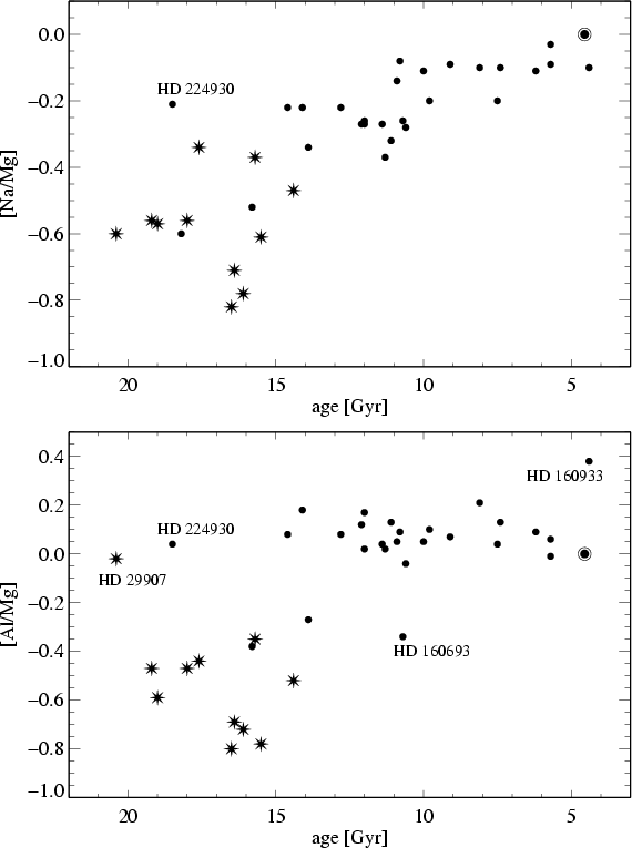	Figure 11: Correlation between abundance ratios and stellar ages. Symbols are the same as in Fig. 6.
Open with DEXTER

   
6 Discussion and conclusions

The small number of stars analyzed here already allows a surprising variety of results to be noted. This depends on an a posteriori reselection of the "typical'' sample stars. Whereas our criteria for this process can be formulated clearly, we admit that such an iterative selection method may not be fully accepted. Our justification is the existence of a surprisingly large fraction of stars with peculiarities such as

• binaries of types SB1 and SB2,
• active chromospheres,
• peculiar abundances or abundance ratios.

Since deviating abundance ratios lead to the most questionable rejection process, we identify here only one such object, HD 74000, known since long for its extreme nitrogen overabundance. In our analysis this is accompanied by exceptional abundances of both Na and Al. The origin of such an abundance pattern will therefore not be discussed here. Mashonkina et al. (2003) have shown that there are other halo stars with similar properties and somewhat peculiar r-process abundances.

As a result our original sample of 38+14 stars, already reduced to 27+11 stars in Sect. 2, will be reduced once more to exclude from the discussion of a clean sample the binaries HD 200580, HD 224930, HD 29907, and the peculiar star HD 74000. Figures 6 to 9, and 11 should therefore be corrected correspondingly.

6.1 NLTE and abundances

The abundance analyses of all elements included here have once again clearly indicated the importance of NLTE when analyzing the stellar spectra. This does not only hold for the abundance analyses themselves, which often are performed only as equivalent width analyses, irrespective of whether the synthesized profiles have anything in common with the observed spectra. Taking care of accurate profile fits, our abundance results are summarized in Fig. 12, which outlines the increase of the differences between LTE and NLTE analyses with decreasing metal abundance, as predicted. We emphasize here again, that our NLTE calculations are conservative in that we have used the typical free parameter, the collision factor $S_{\!\!\rm H}$, to force the abundances of all lines analyzed to a common value (minimizing abundance scatter). Moreover, the full system of equations and parameters simultaneously fits the solar spectrum.

It is also important to realize that the "scatter'' seen in Fig. 12 is not an artefact of an uncertain abundance determination. Carefully identifying the outliers such as G170-56 with an Al abundance difference of 0.6, it becomes evident that the difference between LTE and NLTE abundances is not only a matter of stellar parameters such as $T_{\rm eff}$, $\log g$, and perhaps [Fe/H], but it also depends on the Al abundance itself. Therefore any table giving such correction values would have to be multi-dimensional.

	Figure 12: Difference of element abundance ratios calculated under NLTE and LTE assumptions and displayed in Fig. 6 (see text).
Open with DEXTER

There are, however, some general trends. Most important is the opposite behaviour of Na and Al, which is of course a result of the different atomic structure, Na I being overpopulated by cascades of recombining electrons, whereas Al I is strongly depopulated by photoionization. These effects have been discussed in Sect. 4, and populations of these types are seen in Figs. 4 and 5. In the cool region of the metal-poor HR diagram all abundances of Na and Al must be corrected for the NLTE departures.

   
6.2 Population membership of individual stars

One of the more ambitious goals of this investigation is to identify single stars as members of a population. It is not clear at present, whether the very concept of populations tells us much about Galactic evolution or perhaps only summarizes a few mean properties acquired during various proto-Galactic or later merging processes. It has been noted repeatedly that kinematic data alone do not allow the unambiguous identification of a stellar population. In particular the overlap between halo and thick disk stars has not yet been fully evaluated, and Fig. 9 does not suggests a clear limit of V velocities either. The original classification of populations by their space velocities is therefore almost exclusively of statistical value. The work of Edvardsson et al. (1993), mainly confined to what we still address as the thin disk, has shown that the overall metal abundance represented by [Fe/H] is an insufficient indicator of most criteria of Galactic evolution. This is probably due to inhomogeneous star formation, which may be an order of magnitude more important for the short time intervals encountered during the evolution of thick disk or halo. Figure 6 therefore does not reveal too much of a population structure except that it helps to identify some outliers, here in particular G170-56.

Figure 7 instead allows to note some more important abundance trends. One is the gradual decline of [Na/Mg] with [Mg/Fe], irrespective of the stars being thin or thick disk members. It is not seen as clearly in Figs. 9 or 11. Thus it is more a global correlation that represents nucleosynthesis under quite different conditions. It has to be confronted with the striking difference in [Na/Mg] when comparing (thick) disk with halo stars at the same [Mg/Fe] ratio. There is no such trend with [Mg/Fe] among the [Al/Mg] abundance ratios of the (thick) disk stars, all of which seem to have within a very small scatter the same [Al/Mg] ratio. Then, if ²³Na and ²⁷Al are secondary elements that require the pre-existence of metals, why are they not built up in the same way under disk evolution conditions which may provide the continuous enrichment of Fe/Mg by SNe Ia and thus increase the overall metal abundance? The [Al/Na] ratio emphasizes this problem, with even halo stars showing a solar abundance ratio, but the disk stars (with many of them belonging to the thick disk) cluster around [Al/Mg] = 0.3, although with considerable scatter.

The comparison of [Na/Mg] and [Al/Mg] in Fig. 7 could tell us that hydrostatic carbon and neon burning in (thick) disk stars result from two different sites of nucleosynthesis or at least different masses of the SN II progenitors. A similar scenario has been investigated by Tsujimoto et al. (2002) who have tried to account for the strong scatter of [Na/Mg] and [Al/Mg] ratios they found in the literature. Though that scatter is largely an artefact from the LTE assumption underlying all those analyses or from the various methods of determining stellar parameters, the overall trends seem to be well reproduced assuming the local propagation of synthesized material through adjacent SN shells, in which new stellar generations are initiated. While the yields of both Na and Al in type II supernovae are under debate (Woosley & Weaver 1995; Umeda et al. 2000), it seems that such a model environment for chemical evolution is able to explain the different abundance ratios of Na/Mg and Al/Mg for [Mg/H] > -2. Both [Na/Mg] and [Al/Mg] in the (generally more metal-poor) halo stars represent a significant even-odd effect, the amount of which is somewhere between the results of zero-metal supernovae of type II (Woosley & Weaver 1995) and the production factors of very massive population III stars (Heger & Woosley 2002). According to their investigation population III stars between 40 and 150 $M_\odot$ end in a black hole and do not contribute to chemical evolution. Whereas the synthesis of Na in the disk populations can be explained by gradual enrichment including SN Ia, the constant solar [Al/Mg] in both thin and thick disk remains a puzzle. Timmes et al. (1995) predict an [Al/Mg] ratio gradually increasing from -0.4 in the metal-rich halo to -0.3 in the early thick disk with a further increase to +0.2 at solar metallicity. Our high level of Al abundance ratios in the thick and thin disk, seen also in Edvardsson et al. (1993), is at variance with that prediction. It may require some fine-tuning of preferably discontinuous and/or time-dependent initial mass functions to produce our observed Al/Mg ratio.

	Figure 13: Gap in metal abundance [Fe/H] and abundance ratio [Al/Mg], where no star is found. Such a plot may help to identify population membership.
Open with DEXTER

Aside from chemical evolution considerations it is the [Al/Mg] abundance ratio that could open a second door to population membership identification in very much the same way as [Mg/Fe] was used to discriminate between thin and thick disk (Fuhrmann 1998). For this purpose we consult the correlations of [Al/Mg] with [Mg/Fe] (Fig. 7), the Galactic V velocity (Fig. 9), and the stellar ages (Fig. 11). We must admit that the gap in [Al/Mg] between -0.3 and 0.0 is not yet fully convincing because the sample is still very small, in particular in the range of metal abundances between $\rm [Fe/H] = -1.3$ and -0.8, which shows a similar gap. Such a gap in [Fe/H] is also found in the results of Prochaska et al. (2000). Whether the gap is really existing or only an artefact of small sample statistics, it is important to note that the [Al/Mg] abundance ratios of both disk and halo-type subsamples do not fill in. Thus, halo and disk populations appear to be well separated when they are plotted as a function of the metal abundance [Fe/H] (Fig. 13). In two of the diagrams (Figs. 7 and 9) there is considerable overlap between either [Mg/Fe] or velocity component V. It is only the overall metal abundance and perhaps the stellar ages that seem to separate halo and disk components in a similar way as the [Al/Mg] ratio. Assuming for the moment that the gap in [Al/Mg] were real, it is still necessary to identify the nature of a few outliers that seem to spoil the correlation. We have commented on the binary stars above, so we emphasize only that except for HD 29907 all bona fide halo stars are found between $\rm [Al/Mg] \sim -0.8$ and -0.4, where the scatter of the results is beyond any errors of the spectral analyses. Of course, even more metal-poor stars may show even lower [Al/Mg] ratios.

There are, however, three stars out of our less metal-poor sample that have [Al/Mg] ratios near the upper edge of the typical halo sample (G188-22, HD 160693) or even somewhat above (G170-56). Whereas G188-22 seems to have halo properties when kinematics and age are inspected, HD 160693 is a different case. Its [Mg/Fe] ratio documents that this star must have been formed from matter recycled only in SN II, but its age is roughly 4 to 5 Gyrs less than that of typical halo stars separating it from the halo in terms of Galactic evolution. HD 160693 could therefore be a former member of an accreted dwarf galaxy or globular cluster. G170-56 on the other side has a typical thin disk [Mg/Fe] ratio which requires that its formation must have been based on matter recycled in SN Ia. We note that stars like G170-56 are not found in the thick disk either. Therefore we should rule out its membership in both thick disk and halo. Its exceedingly low Na and Al abundances are certainly surprising in view of the retrograde Galactic orbit. Quite probably, also G242-4 would have to be attributed to the halo, although its Al abundance could not be analyzed here.

A number of additional comments refer to population membership. Most of them have to do with kinematical properties of the stars. A star like HD 97320 would never be classified as a halo star from kinematics alone; both abundance ratios and age clearly show that it must belong at least to a pre-disk origin. HD 148816 is the kinematical counterpart of HD 97320. With a retrograde orbit this star seems to have more in common with G170-56 than any other star in the sample, although its [Al/Mg] and [Na/Mg] are atypical for the high [Mg/Fe] ratio. At the same time HD 148816 has only a moderate metal deficiency of -0.78 which, for a halo star, would also be at an extreme end. In summary it seems that roughly two thirds of the remaining stars on our two lists can be attributed to the thick disk or halo populations, whereas some of the other stars cannot be classified in such a simple way. The important question whether our Galaxy can be composed of three homogeneous populations will have to await more results from future spectral analyses. At present the identification of population membership is based essentially in Fig. 13, where halo stars and disk stars seem well separated at $\rm [Fe/H] \sim -1.0$, $\rm [Al/Mg] \sim -0.15$. A similar boundary is found at [Na/Mg] $\sim -0.4$. The discrimination between thin and thick disk stars follows Fuhrmann (1998) using [Mg/Fe] = 0.25 as a boundary. This classification scheme is reproduced in the last column of Table 4.

6.3 The age coordinate

Stellar ages displayed in Fig. 11, are not only very high and therefore unrealistic as absolute data but also do not exhibit a clear separation between thick and thin disk as was suggested by Fuhrmann (2000). Fuhrmann notes an age gap between roughly 9 and 12 Gyrs, which in fact refers to the age interval that is most densely populated in our sample. This could in part be due to the use of different evolutionary tracks, but to first order one would expect a shift of ages. Figure 11 shows that the region of the proposed age gap between thin and thick disk is populated by a mixture of stars identified both as thin or thick disk. The age overlap is near 2 Gyrs, and it is hard to think of any simple combination of analysis errors that could produce it. Unfortunately, Fuhrmann's and our work have only one star in common, HD 204155, which is outside the critical age range. Even accepting a misidentification for many stars in that range, there would be no age gap.

The question arises therefore, whether the age itself is a good population identifier. It may be that the stars filling in the gap that Fuhrmann claims to have detected are (a) no members of our standard populations, and/or (b) did not appear in the small local volume of Fuhrmann's sample. In the first case, quite a large fraction of our stars must come from separate evolutionary processes such as merging or tidal disruption of galaxies or clusters; stars like that could also belong to the intermediate population with [Mg/Fe] around 0.2, which stands out from the trends in thin and thick disk. In the second case, Fuhrmann's small local volume, although statistically complete, might not be representative for more extended parts of the Milky Way. Of course, it would be much more likely that our sample is not representative.

We note, however, that the age limit between halo and thick disk population seems to be much better defined in Fig. 11. In our analysis it lies near 14 Gyr, but that value could be reduced when evolutionary tracks with diffusion will become available.

The results presented in this paper are therefore not yet robust enough to warrant further speculations. Work extending the data set is under way.

Acknowledgements

This project was supported by the Deutsche Forschungsgemeinschaft (DFG) under grants Ge 490/26-1, 490/27-1, 490/28-1 and 490/30-1, and by the National Natural Science Foundation of China (NSFC) under grants 10173014 and NKBRSF G1999075406. We gratefully mention the help of Keith Butler and Andreas Korn. Don VandenBerg kindly supported us making available his most recent calculations of stellar evolution.

References

 
• Ali, A. W., & Griem, H. R. 1965, Phys. Rev. A, 140, 1044 In the text  
• Ali, A. W., & Griem, H. R. 1966, Phys. Rev., 144, 366 In the text NASA ADS  
• Alonso, A., Arribas, S., & Martínez-Roger, C. 1995, A&A, 297, 197 In the text NASA ADS  
• Alonso, A., Arribas, S., & Martínez-Roger, C. 1996, A&AS, 117, 227 In the text NASA ADS  
• Anders, E., & Grevesse, N. 1989, Geochim. Cosmochim. Acta, 53, 197 In the text NASA ADS  
• Anstee, S. D., & O'Mara, B. J. 1991, MNRAS, 253, 549 In the text NASA ADS  
• Anstee, S. D., & O'Mara, B. J. 1995, MNRAS, 276, 859 In the text NASA ADS  
• Arnett, D. 1996, Supernovae and Nucleosynthesis (New Jersey: Princeton Univ. Press, Princeton) In the text  
• Barklem, P. S., Piskunov, N., & O'Mara, B. J. 2000, A&A, 363, 1091 In the text NASA ADS  
• Baumüller, D., & Gehren, T. 1996, A&A, 307, 961 In the text NASA ADS  
• Baumüller, D., & Gehren, T. 1997, A&A, 325, 1088 In the text NASA ADS  
• Baumüller, D., Butler, K., & Gehren, T. 1998, A&A, 338, 637 In the text NASA ADS  
• Bautista, M. A. 1997, A&AS, 122, 167 In the text NASA ADS  
• Bergbusch, P. A., & VandenBerg, D. A. 1992, ApJS, 81, 163 In the text NASA ADS  
• Bernkopf, J., Fiedler, A., & Fuhrmann, K. 2001, ASP Conf. Ser., 245, 207 In the text  
• Binney, J., & Merrifield, M. 1998, Galactic Astronomy (New Jersey: Princeton Univ. Press, Princeton) In the text  
• Butler, K. 1993, unpublished In the text  
• Butler, K., & Giddings, J. 1985, Newsletter on the analysis of astronomical spectra No. 9, University of London In the text  
• Butler, K., Mendoza, C., & Zeippen, C. J. 1993, J. Phys. B, 26, 4409 In the text NASA ADS  
• Carbon, D. F., Barbuy, B., Kraft, R. P., et al. 1987, PASP, 99, 335 In the text NASA ADS  
• Carney, B. W., & Latham, D. W. 1987, AJ, 93, 116 In the text NASA ADS  
• Carretta, E., Gratton, R. G., & Sneden, C. 2000, A&A, 356, 238 In the text NASA ADS  
• Chen, Y. Q., Nissen, P. E., Zhao, G., Zhang, H. W., & Benoni, T. 2000, A&AS, 141, 491 In the text NASA ADS  
• Clausen, J. V., Larsen, S. S., Garcia, J. M., et al. 1997, A&AS, 122, 559 In the text NASA ADS  
• Cowan, J. J., Sneden, C., Burles, S., et al. 2002, ApJ, 572, 861 In the text NASA ADS  
• Drawin, H. W. 1968, Z. Phys., 211, 404 In the text  
• Drawin, H. W. 1969, Z. Phys., 225, 483 In the text  
• Edvardsson, B., Anderson, J., Gustafsson, B., et al. 1993, A&A, 275, 101 In the text NASA ADS  
• ESA 1997, The Hipparcos and Tycho Catalogues, ESA SP-1200 In the text  
• Fuhrmann, K. 1998, A&A, 338, 161 In the text NASA ADS  
• Fuhrmann, K. 2000, in The First Stars. Proc. MPA/ESO Workshop, ed. A. Weiss, T. G. Abel, & V. Hill (Springer), 68 In the text  
• Fuhrmann, K. 2002, New Astr., 7, 161 In the text NASA ADS  
• Fuhrmann, K., Axer, M., & Gehren, T. 1993, A&A, 271, 451 In the text NASA ADS  
• Fuhrmann, K., Axer, M., & Gehren, T. 1994, A&A, 285, 585 In the text NASA ADS  
• Fulbright, J. P. 2000, AJ, 120, 1841 In the text NASA ADS  
• Fulbright, J. P. 2002, AJ, 123, 404 In the text NASA ADS  
• Gehren, T., Butler, K., Mashonkina, L., et al. 2001, A&A, 366, 981 In the text NASA ADS  
• Gilmore, G., & Reid, N. 1983, MNRAS, 202, 1025 In the text NASA ADS  
• Goldberg, D., Mazeh, T., Latham, D. W., et al. 2002, AJ, 124, 1132 In the text NASA ADS  
• Gratton, R. G., Carretta, E., Eriksson, K., et al. 1999, A&A, 350, 955 In the text NASA ADS  
• Greenstein, J. L., & Saha, A. 1986, ApJ, 304, 721 In the text NASA ADS  
• Heger, A., & Woosley, S. E. 2002, ApJ, 567, 532 In the text NASA ADS  
• Hünsch, M., Schmitt, J. H. M. M., Sterzik, M. F., et al. 1999, A&AS, 135, 319 In the text NASA ADS  
• Kurucz, R. L. 1992, Rev. Mex. Astron. Astrof., 23, 45 In the text NASA ADS  
• Kurucz, R. L., Furenlid, I., Brault, J., et al. 1984, Solar Flux Atlas from 296 to 1300 nm, Kitt Peak National Solar Observatory In the text  
• Latham, D. W., Mazeh, T., Carney, B. W., et al. 1988, AJ, 96, 567 In the text NASA ADS  
• Latham, D. W., Stefanik, R. P., Torres, G., et al. 2002, AJ, 124, 1144 In the text NASA ADS  
• Lindgren, H., & Ardeberg, A. 1996, A&AS, 119, 25 In the text NASA ADS  
• Mashonkina, L. I., Gehren, T., & Bikmaev, I. F. 1999, A&A, 343, 519 In the text NASA ADS  
• Mashonkina, L., Gehren, T., Travaglio, C., et al. 2003, A&A, 397, 275 In the text NASA ADS  
• Mason, B. D., Hartkopf, W. I., Holdenried, E. R., et al. 2001, AJ, 121, 3224 In the text NASA ADS  
• McWilliam, A., Preston, G. W., Sneden, C., et al. 1995, AJ, 109, 2757 In the text NASA ADS  
• McWilliam, A. 1997, ARA&A, 35, 503 In the text NASA ADS  
• Nidever, D. L., Marcy, G. W., Butler, R. P., et al. 2002, ApJS, 141, 503 In the text NASA ADS  
• Nissen, P. E., Primas, F., Asplund, M., et al. 2002, A&A, 390, 235 In the text NASA ADS  
• Norris, J., Bessell, M., & Pickles, A. J. 1985, ApJS, 58, 463 In the text NASA ADS  
• Pfeiffer, M., Frank, C., Baumüller, D., et al. 1998, A&AS, 130, 381 In the text NASA ADS  
• Pilachowski, C. A., Sneden, C., & Kraft, R. P. 1996, AJ, 111, 1689 In the text NASA ADS  
• Prochaska, J. X., Naumov, S. O., Carney, B. W., et al. 2000, AJ, 120, 2513 In the text NASA ADS  
• Reetz, J. K. 1993, priv. communication In the text  
• Richard, O., Michaud, G., & Richer, J. 2002, ApJ, 568, 979 In the text NASA ADS  
• Roman, N. 1950, ApJ, 112, 554 In the text NASA ADS  
• Ryan, S. G., Norris, J. E., & Beers, T. C. 1996, ApJ, 471, 254 In the text NASA ADS  
• Rybicki, G. B., & Hummer, D. G. 1991, A&A, 245, 171 In the text NASA ADS  
• Rybicki, G. B., & Hummer, D. G. 1992, A&A, 262, 209 In the text NASA ADS  
• Sandage, A., & Fouts, G. 1987, AJ, 93, 74 In the text NASA ADS  
• Seaton, M. J. 1962, in Atomic and Molecular Processes (New York: Acad. Press) In the text  
• Smith, G., & Churchill, C. 1998, MNRAS, 297, 388 In the text NASA ADS  
• Spergel, D. N., Verde, L., Peiris, H. V., et al. 2003 [astro-ph/0302209] In the text  
• Timmes, F. X., Woosley, S. E., & Weaver, T. A. 1995, ApJS, 98, 617 In the text NASA ADS  
• Tomkin, J., Lambert, D. L., & Balachandran, S. 1985, ApJ, 290, 289 In the text NASA ADS  
• Tomkin, J., Lemke, M., Lambert, D. L., et al. 1992, AJ, 104, 1568 In the text NASA ADS  
• Tsujimoto, T., Shigeyama, T., & Yoshii, Y. 2002, ApJ, 565, 1011 In the text NASA ADS  
• Umeda, H., Nomoto, K., & Nakamura, T. 2000, in The First Stars, ed. A. Weiss, T. Abel, & V. Hill (Heidelberg: Springer), 150 In the text  
• Underhill, A. B. 1963, Publ. Dom. Astr. Obs., 12, 159 In the text NASA ADS  
• VandenBerg, D. A., Swenson, F. J., Rogers, F. J., et al. 2000, ApJ, 532, 430 In the text NASA ADS  
• VandenBerg, D. A., Richard, O., Michaud, G., et al. 2002, ApJ, 571, 487 In the text NASA ADS  
• van Regemorter, H. 1962, ApJ, 136, 906 In the text NASA ADS  
• Woosley, S. E., & Weaver, T. A. 1995, ApJS, 101, 181 In the text NASA ADS  
• Zhao, G., Butler, K., & Gehren, T. 1998, A&A, 333, 219 In the text NASA ADS  
• Zhao, G., & Gehren, T. 2000, A&A, In the text