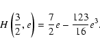
The 3:2 spin-orbit resonance between the rotational and orbital motions of Mercury (the periods are
A&A 413, 381-393 (2004)
DOI: 10.1051/0004-6361:20031446
N. Rambaux - E. Bois
Observatoire Aquitain des Sciences de l'Univers, Université Bordeaux 1, UMR CNRS/INSU 5804, BP 89, 33270 Floirac, France
Received 16 June 2003 / Accepted 13 August 2003
Abstract
The 3:2 spin-orbit resonance between the rotational and orbital motions of
Mercury (the periods are
![]() and
and
![]() days respectively) results from a functional dependance of the tidal friction
adding to a non-zero eccentricity and a permanent asymmetry in the equatorial
plane of the planet. The upcoming space missions, MESSENGER and
BepiColombo with onboard instrumentation capable of measuring the rotational
parameters stimulate the objective to reach an accurate theory of the rotational
motion of Mercury. For obtaining the real motion of Mercury, we have
used our BJV model of solar system integration including the coupled spin-orbit
motion of the Moon. This model, expanded in a relativistic framework, had been
previously built in accordance with the requirements of the Lunar Laser Ranging
observational accuracy. We have extended the BJV model by generalizing the
spin-orbit couplings to the terrestrial planets (Mercury, Venus, Earth, and Mars).
The updated model is called SONYR (acronym of Spin-Orbit N-BodY Relativistic model).
As a consequence, the SONYR model gives an accurate simultaneous integration of the
spin-orbit motion of Mercury. It permits one to analyze the different families
of rotational librations and identify their causes such as planetary interactions or the
parameters involved in the dynamical figure of the planet. The spin-orbit motion of
Mercury is characterized by two proper frequencies (namely
days respectively) results from a functional dependance of the tidal friction
adding to a non-zero eccentricity and a permanent asymmetry in the equatorial
plane of the planet. The upcoming space missions, MESSENGER and
BepiColombo with onboard instrumentation capable of measuring the rotational
parameters stimulate the objective to reach an accurate theory of the rotational
motion of Mercury. For obtaining the real motion of Mercury, we have
used our BJV model of solar system integration including the coupled spin-orbit
motion of the Moon. This model, expanded in a relativistic framework, had been
previously built in accordance with the requirements of the Lunar Laser Ranging
observational accuracy. We have extended the BJV model by generalizing the
spin-orbit couplings to the terrestrial planets (Mercury, Venus, Earth, and Mars).
The updated model is called SONYR (acronym of Spin-Orbit N-BodY Relativistic model).
As a consequence, the SONYR model gives an accurate simultaneous integration of the
spin-orbit motion of Mercury. It permits one to analyze the different families
of rotational librations and identify their causes such as planetary interactions or the
parameters involved in the dynamical figure of the planet. The spin-orbit motion of
Mercury is characterized by two proper frequencies (namely
![]() yrs and
yrs and
![]() yrs) and its 3:2 resonance presents a second synchronism which can be understood as
a spin-orbit secular resonance (
yrs) and its 3:2 resonance presents a second synchronism which can be understood as
a spin-orbit secular resonance (
![]() yrs). A new determination
of the mean obliquity is proposed in the paper. By using the SONYR model, we
find a mean obliquity of 1.6 arcmin. This value is consistent with the Cassini
state of Mercury. Besides, we identify in the Hermean librations the impact of
the uncertainty of the greatest principal moment of inertia (
yrs). A new determination
of the mean obliquity is proposed in the paper. By using the SONYR model, we
find a mean obliquity of 1.6 arcmin. This value is consistent with the Cassini
state of Mercury. Besides, we identify in the Hermean librations the impact of
the uncertainty of the greatest principal moment of inertia (
![]() )
on the obliquity and
on the libration in longitude (2.3 milliarcsec and 0.45 arcsec respectively for an increase of 1
)
on the obliquity and
on the libration in longitude (2.3 milliarcsec and 0.45 arcsec respectively for an increase of 1![]() on the
on the
![]() value). These determinations prove to be suitable for providing
constraints on the internal structure of Mercury.
value). These determinations prove to be suitable for providing
constraints on the internal structure of Mercury.
Key words: methods: numerical - celestial mechanics - planets and satellites: individual: Mercury
Before 1965, the rotational motion of Mercury was assumed to be
synchronous with its orbital motion. In 1965, Pettengill & Dyce discovered
a 3:2 spin-orbit resonance state by using Earth-based radar
observations (the Mercury's rotation period is
![]() days
while the orbital one is
days
while the orbital one is
![]() days). This surprising resonance
results from a non-zero eccentricity and a permanent asymmetry in
the equatorial plane of the planet. In addition, the 3:2 resonance strongly
depends on the functional dependance of the tidal torque on the rate of the
libration in longitude. Moreover the 3:2 resonance state is preserved by the
tidal torque (Colombo & Shapiro 1966). The main dynamical features of
Mercury have been established during the 1960s in some pioneer works such
as Colombo (1965), Colombo & Shapiro (1966), Goldreich & Peale (1966)
and Peale (1969). Goldreich & Peale (1966) notably studied the probability of
resonance capture and showed that the 3:2 ratio is the only possible one for a
significant probability of capture. In addition, in a tidally evolved system, the
spin pole is expected to be trapped in a Cassini state (Colombo 1966; Peale 1969,
1973). The orbital and rotational parameters are indeed matched in such a way
that the spin pole, the orbit pole, and the solar system invariable pole
remain coplanar while the spin and orbital poles precess. The reader may find in
Balogh & Campieri (2002) a review report on the present knowledge of Mercury
whose the interest is nowadays renewed by two upcoming missions:
MESSENGER (NASA, Solomon et al. 2001) and BepiColombo (ESA, ISAS,
Anselin & Scoon 2001).
days). This surprising resonance
results from a non-zero eccentricity and a permanent asymmetry in
the equatorial plane of the planet. In addition, the 3:2 resonance strongly
depends on the functional dependance of the tidal torque on the rate of the
libration in longitude. Moreover the 3:2 resonance state is preserved by the
tidal torque (Colombo & Shapiro 1966). The main dynamical features of
Mercury have been established during the 1960s in some pioneer works such
as Colombo (1965), Colombo & Shapiro (1966), Goldreich & Peale (1966)
and Peale (1969). Goldreich & Peale (1966) notably studied the probability of
resonance capture and showed that the 3:2 ratio is the only possible one for a
significant probability of capture. In addition, in a tidally evolved system, the
spin pole is expected to be trapped in a Cassini state (Colombo 1966; Peale 1969,
1973). The orbital and rotational parameters are indeed matched in such a way
that the spin pole, the orbit pole, and the solar system invariable pole
remain coplanar while the spin and orbital poles precess. The reader may find in
Balogh & Campieri (2002) a review report on the present knowledge of Mercury
whose the interest is nowadays renewed by two upcoming missions:
MESSENGER (NASA, Solomon et al. 2001) and BepiColombo (ESA, ISAS,
Anselin & Scoon 2001).
Our work deals with the physical and dynamical causes that contribute to induce librations around an equilibrium state defined by a Cassini state. In order to wholly analyze the spin-orbit motion of Mercury and its rotational librations, we used a gravitational model of the solar system including the Moon's spin-orbit motion. The framework of the model has been previously constructed by Bois, Journet & Vokrouhlický (BJV model) in accordance with the requirements of Lunar Laser Ranging (LLR thereafter) observational accuracy (see for instance a review report by Bois 2000). The approach of the model consists in integrating the N-body problem on the basis of the gravitation description given by the Einstein's general relativity theory according to a formalism derived from the first post-Newtonian approximation level. The model is solved by modular numerical integration and controlled in function of the different physical contributions and parameters taken into account. We have extended this model to the integration of the rotational motions of the terrestrial planets (Mercury, Venus, Earth, and Mars) including their spin-orbit couplings. The updated model is then called SONYR (acronym of Spin-Orbit N-bodY Relativistic model). As a consequence, using SONYR, the N-body problem for the solar system and the spin motion of Mercury are simultaneously integrated. Consequently we may analyze and identify the different families of Hermean rotational librations with the choice of the contributions at our disposal.
Starting with the basic spin-orbit problem according to Goldreich & Peale (1966), we have computed a surface of section for the Mercury's rotation showing its very regular behavior. We have calculated again the proper frequency for the spin-orbit resonance state of Mercury. Using our model, an important part of the present study deals with the main perturbations acting on the spin-orbit motion of Mercury such as the gravitational figure of the planet as well as the planetary effects and their hierarchy. A detailed analysis of the resulting rotational librations due to these effects is presented and described in the paper. A new determination of the Hermean mean obliquity is also proposed. Moreover, we identify in the Hermean librations the impact of the variation of the greatest principal moment of inertia on the instantaneous obliquity and on the libration in longitude. Such a signature gives noticeable constraints on the internal structure of Mercury.
According to Goldreich & Peale (1966), we consider the spin-orbit
motion of Mercury with its spin axis normal to the orbital plane.
The orbit is assumed to be fixed and unvariable (semi-major
axis a and its eccentricity e). The position of Mercury is determined by
its instantaneous radius r while its rotational orientation is specified by the
angle ![]() .
The orbital longitude is specified by the true anomaly f while the angle
.
The orbital longitude is specified by the true anomaly f while the angle
![]() measures the angle between
the axis of least moment of inertia of Mercury and the Sun-to-Mercury line
(see Fig. 1). According to these assumptions, the dynamical
problem of the spin-orbit motion of Mercury is reduced to a one-dimensional
pendulum-like equation as follows:
measures the angle between
the axis of least moment of inertia of Mercury and the Sun-to-Mercury line
(see Fig. 1). According to these assumptions, the dynamical
problem of the spin-orbit motion of Mercury is reduced to a one-dimensional
pendulum-like equation as follows:
| |
Figure 1:
Geometry of the spin-orbit coupling problem.
|
| Open with DEXTER | |
![\begin{figure}
\par\includegraphics[width=18cm]{fig2.eps} %\end{figure}](/articles/aa/full/2004/01/aa4114/img30.gif) |
Figure 2:
Surface of section of the Mercury's spin-orbit
coupling (
|
| Open with DEXTER | |
In order to know the structure of the phase space of the Mercury's
rotation, a surface of section for its spin-orbit coupling is very
useful. Let be
![]() the asphericity of the
Mercury's dynamical figure combining the principal moments of inertia
A, B, and C. Equation (1) becomes:
the asphericity of the
Mercury's dynamical figure combining the principal moments of inertia
A, B, and C. Equation (1) becomes:
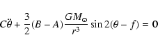
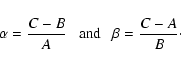
According to the Chirikov resonance overlap criterion (1979), the chaotic
behavior appears when the asphericity of the body is larger than the
following critical value:
 |
(3) |
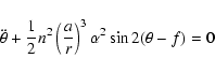
From Eq. (1), it is possible to obtain an integrable
approximated equation using the spin-orbit resonance, the spin rate
![]() being commensurable with the mean orbital motion n. Following
Murray & Dermott (2000), by introducing a new variable
being commensurable with the mean orbital motion n. Following
Murray & Dermott (2000), by introducing a new variable
![]() where p parametrizes the resonance ratio (
where p parametrizes the resonance ratio (
![]() in the case of Mercury), one may expand the equation in form-like Poisson
series. Taking into account that
in the case of Mercury), one may expand the equation in form-like Poisson
series. Taking into account that
![]() ,
one averages all the
terms over one orbital period, and finally obtain the
following equation:
,
one averages all the
terms over one orbital period, and finally obtain the
following equation:
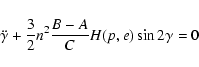
 |
(5) |
![\begin{displaymath}\omega_{0} = n \left[ 3 \frac{B-A}{C} \vert H(p,e) \vert
\right]^{\frac{1}{2}} \\
\end{displaymath}](/articles/aa/full/2004/01/aa4114/img46.gif) |
(6) |
![\begin{figure}
\par\includegraphics[angle=-90,width=8.4cm,clip]{Difflib.ps}
\end{figure}](/articles/aa/full/2004/01/aa4114/img47.gif) |
Figure 3: The spin-orbit solution of Mercury in the planar case (Eq. (7)) plotted over 250 days. Arcseconds are on the vertical axis and days on the horizontal axis. Short-term librations have a period of 87.969 days (the orbital period of Mercury) and 42 as of amplitude. |
| Open with DEXTER | |
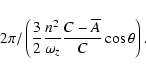
Balogh & Giamperi (2002) developed Eq. (2) and obtained
the following expression:
However, the above equations describe a spin-orbit motion of Mercury where the spin axis is normal to the orbital plane while the orbital motion is Keplerian.
In order to wholly analyze the spin-orbit motion of Mercury and its rotational librations, we have enlarged a gravitational model (called BJV) of the solar system including the Moon's spin-orbit motion. The accurate theory of the Moon's spin-orbit motion, related to this BJV model, was constructed by Bois, Journet & Vokrouhlický in accordance with the high accuracy of the LLR observations (see previous papers: Bois et al. 1992; Bois & Journet 1993; Bois & Vokrouhlický 1995; Bois et al. 1996; Bois & Girard 1999). The approach of the BJV model consists in integrating the N-body problem (including translational and rotational motions) on the basis of the gravitation description given by the Einstein's general relativity theory. The equations have been developped in the DSX formalism presented in a series of papers by Damour et al. (Damour et al. 1991, 1992, 1993, 1994). For purposes of celestial mechanics, to our knowledge, it is the most suitable formulation of the post-Newtonian (PN) theory of motion for a system of N arbitrary extended, weakly self-graviting, rotating and deformable bodies in mutual interactions. The DSX formalism, derived from the first post-Newtonian approximation level, gives the post-Newtonian representation of the translational motions of the bodies as well as their rotational ones with respect to the locally transported frames with the bodies.
Gravitational fields of the extended bodies are parameterized in
multipole moment expansions:
![]() define the mass and spin
Blanchet-Damour multipoles characterizing the PN gravitational field of
the extended bodies while
define the mass and spin
Blanchet-Damour multipoles characterizing the PN gravitational field of
the extended bodies while
![]() are tidal gravitoelectric
and gravitomagnetic PN fields. Because we do not dispose of dynamical
equations for the quadrupole moments
are tidal gravitoelectric
and gravitomagnetic PN fields. Because we do not dispose of dynamical
equations for the quadrupole moments
![]() ,
and although the
notion of rigidity faces conceptual problems in the theory of relativity,
we have adopted the "rigid-multipole'' model of the extended bodies as
known from the Newtonian approach. Practically this is acceptable since
the relativistic quadrupole contributions are very small. Consequently
and because it is conventional in geodynamical research to use spherical
harmonics analysis of the gravitational fields with the corresponding
notion of harmonic coefficients
,
and although the
notion of rigidity faces conceptual problems in the theory of relativity,
we have adopted the "rigid-multipole'' model of the extended bodies as
known from the Newtonian approach. Practically this is acceptable since
the relativistic quadrupole contributions are very small. Consequently
and because it is conventional in geodynamical research to use spherical
harmonics analysis of the gravitational fields with the corresponding
notion of harmonic coefficients
![]() ,
the quadrupole
moments
,
the quadrupole
moments
![]() have been expressed in those terms, according to
reasons and assumptions given in Bois & Vokrouhlický (1995).
Gravitational figures as well as the figure-figure interactions of
the bodies are then represented by expansions in spherical harmonics
(Borderies 1978; Shutz 1981). Moreover, internal structures of solid
deformable bodies, homogeneous or with core-mantle interfaces, are
represented by several terms and parameters arising from tidal
deformations of the bodies (both elastic and anelastic). More details
and references on these topics are given in the above quoted papers
related to our works concerning the theory of the Moon's spin-orbit
motion.
have been expressed in those terms, according to
reasons and assumptions given in Bois & Vokrouhlický (1995).
Gravitational figures as well as the figure-figure interactions of
the bodies are then represented by expansions in spherical harmonics
(Borderies 1978; Shutz 1981). Moreover, internal structures of solid
deformable bodies, homogeneous or with core-mantle interfaces, are
represented by several terms and parameters arising from tidal
deformations of the bodies (both elastic and anelastic). More details
and references on these topics are given in the above quoted papers
related to our works concerning the theory of the Moon's spin-orbit
motion.
The BJV model, as described above, has been extended to the spin-orbit integration of the terrestrial planets (Mercury, Venus, Earth, and Mars). This new model is henceforth called SONYR (for Spin-Orbit N-bodY Relativistic model). In the present paper framework, the SONYR model is devoted to the detailed analysis of the complete spin-orbit motion of Mercury.
The simultaneous integration of the solar system, including the Mercury's spin-orbit motion, uses a global reference system given by the solar system barycenter. Nevertheless, let us recall that local dynamically non-rotating frames show a slow (de Sitter) rotation with respect to the kinematically non-rotating frames. As a consequence, the reference frame for the Mercury's rotation is affected by a slow precession of its axes transported with the translational motion of Mercury. In the Earth's case, the de Sitter secular precession of the Earth reference frame is close to 1.92 as/cy (see Fukushima 1991; Bizouard et al. 1992; Bois & Vokrouhlický 1995). Consequently, the real rotation of Mercury has not to be expressed in an inertial system fixed in space, but in a local dynamically non-rotating frame fallen down in the gravitational field of the Sun. Because of the proximity of Mercury to the Sun, its de Sitter precession may be expected quite significant.
In the end, the SONYR model and its analysis method take into account (i) the experience in post-Newtonian gravitation in the definition of reference frames required to deal with rotational motions combined with translational ones, and (ii) the modern knowledge of dynamical systems for studiing librations as quasi-periodic solutions according to the axiomatic presented in Bois (1995). We can state that the model is not Newtonian but rather "Newtonian-like'', resulting from truncation of the fully post-Newtonian (DSX) framework. In the present paper, we deal with the Newtonian-like librations (classical physical librations), while the formally relativistic contributions (relativistic librations and de Sitter precession of the Mercury's reference frame) will be analyzed in a forthcoming paper.
Table 1: Our initial conditions at 07.01.1969 (equinox J2000).
The model is solved by modular numerical integration and controlled in function of the different physical contributions and parameters taken into account. The N-body problem (for the translational motions), the rotational motions, the figure-figure and tidal interactions between the required bodies are simultaneously integrated with the choice of the contributions and truncations at our disposal. For instance, the upper limits of the extended figure expansions and mutual interactions may be chosen as follows: up to l=5 in the Moon case, 4 for the Earth, 2 for the Sun while only the Earth-Moon quadrupole-octupole interaction is taken into account (see previous papers). The model has been especially built to favor a systematic analysis of all the effects and contributions. In particular, it permits the separation of various families of librations in the rotational motions of the bodies.
The non-linearity features of the differential equations, the degree of correlation of the studied effect with respect to its neighbors (in the Fourier space) and the spin-orbit resonances (in the Moon and Mercury's cases), make it hardly possible to speak about "pure'' effects with their proper behavior (even after fitting of the initial conditions). The effects are not absolutely de-correlated but relatively isolated. However, the used technique (modular and controlled numerical integration, differentiation method, mean least-squares and frequency analysis) gives the right qualitative behavior of an effect and a good quantification for this effect relative to its neighbors. In the case of the particular status of the purely relativistic effetcs, their quantitative behaviors are beyond the scope of the present paper and will be discussed in a forthcoming work. When a rotational effect is simply periodic, a fit of the initial conditions for a set of given parameters only refines without really changing the effect's behavior. The amplitudes of librations plotted in Figs. 11 and 12 are then slightly upper bounds.
The precision of the model is related to the one required by the theory of the Moon. One of the aims in building the BJV model (at present included inside SONYR) was to take into account all phenomena up to the precision level resulting from the LLR data (i.e. at least 1 cm for the Earth-Moon distance, 1 milliarcsec (mas) for the librations). For reasons of consistency, several phenomena capable of producing effects of at least 0.1 mas had been also modeled (the resulting libration may be at the observational accuracy level). Moreover, in order to justify consistence of the Moon's theory, this one had been adjusted to the JPL ephemeris on the first 1.5 yrs up to a level of a few centimeter residuals. In the other hand, the internal precision of the model is only limited by the numerical accuracy of the integration. Thus, in order to avoid numerical divergence at the level of our tests for Mercury, computations have been performed in quadrupole precision (32 significant figures, integration at a 10-14 internal tolerance).
In order to de-correlate the different librations of Mercury, we use the terminology proposed in Bois (1995), which is suitable for a general and comparative classification of rotational motions of the celestial solid bodies. This terminology derives from a necessary re-arrangement of the lunar libration families due to both progress in the Moon's motion observations (LLR) and modern knowledge of dynamical systems.
Traditionally, the libration mode called physical libration is split up according to the conventional dualism "forced-free''. The forced physical librations are generally related to gravitational causes while the free librations would be departures of the angular position from an equilibrium state. These cuttings out contain ambiguities and redundancies discussed in previous papers (Bois 1995, 2000). Formally, the free librations are periodic solutions of a dynamical system artificially integrable (by a convention of writing related to specific rates of the spin-orbit resonance, for instance 1:1), whereas the forced librations express, in space phase, quasi-periodic solutions around a fixed point (the system is no longer integrable). Moreover, any stable perturbed rotation of celestial solid body contains imbricate librations of different nature, and those are too strongly overlapped to keep the traditional classification.
In the present terminology, the libration nature, its cause and its designation are linked up. Two great libration families serve to define the physical librations, namely the potential librations and the kinetical librations. They simply correspond to a variation energy, potential or kinetical respectively. For libration sub-classes, the designation method is extensive to any identified mechanism (see more details in Bois 1995). The terminology permits easily the separation of various families (see the Moon's case described in a set of previous papers). These librations are called direct when they are produced by torques acting on the body's rotation. They are called indirect when they are produced by perturbations acting on the orbital motion of the body. Indirect librations derive from spin-orbit couplings.
A specificity of the SONYR model with its method of analysis is to isolate the signature of a given perturbation. The SONYR model allows indeed the identification of relationships between causes and effects including interactions between physics and dynamics, such as the dynamical signature of a core-mantle interaction (called centrifugal librations).
In the computations presented in the paper, the required dynamical
parameters and general initial conditions come from the JPL DE405
ephemeris (Standish 1998). However, concerning the parameters related
to the Mercury's rotation (second-degree spherical harmonics C20and C22), which are not included in the JPL ephemeris,
our model uses those given by Anderson et al. (1987) (see
Table 2). Besides, up to now it does not exist any ephemeris
of the Mercury's rotation. As a consequence, to build initial
conditions for the Hermean rotation (described by an Eulerian
sequence of angles ![]() ,
,
![]() and
and ![]() defined below in Sect. 4.1), we use the following principle: assuming the polar axis of
Mercury normal to its orbital plane, we obtain
defined below in Sect. 4.1), we use the following principle: assuming the polar axis of
Mercury normal to its orbital plane, we obtain
![]() and
and
![]() where
where ![]() and i are respectively the ascending node and the inclination
of the orbit of Mercury on the Earth equatorial plane (which is the reference
frame used in the DE405 ephemeris). The long axis of Mercury being pointed
towards the Sun at its periapse allows to fix the
and i are respectively the ascending node and the inclination
of the orbit of Mercury on the Earth equatorial plane (which is the reference
frame used in the DE405 ephemeris). The long axis of Mercury being pointed
towards the Sun at its periapse allows to fix the ![]() angle of
polar rotation. The value of
angle of
polar rotation. The value of
![]() is found in Seidelmann et al. (2002).
We use at last
is found in Seidelmann et al. (2002).
We use at last
![]() and
and
![]() ;
these two variables reach
to mean values generated by the complete spin-orbit problem of Mercury:
;
these two variables reach
to mean values generated by the complete spin-orbit problem of Mercury:
![]() deg/day and
deg/day and
![]() deg/day
respectively. The numerical integrations presented in the paper start from these
initial conditions related to the planar problem for Mercury; they are listed
in Table 1. Departure from the planar case is understood
as the integration of physics included in SONYR.
deg/day
respectively. The numerical integrations presented in the paper start from these
initial conditions related to the planar problem for Mercury; they are listed
in Table 1. Departure from the planar case is understood
as the integration of physics included in SONYR.
In the other hand, for the computations carried out in this paper, the global reference frame O'X'Y'Z' is given by a reference system centered on the solar system barycenter, fixed on the ecliptic plane, and oriented at the equinox J2000. The rotational motion of Mercury is evaluated from a coordinate axis system centered on the Mercury's center of mass Oxyz relative to a local dynamically non-rotating reference frame, OXYZ, whose axes are initially co-linear to those of O'X'Y'Z'. In the framework of the present paper without purely relativistic contributions, let us note that axes of OXYZ remain parallel to those of O'X'Y'Z'.
Table 2: Parameters of Mercury.
Table 3:
Our results for the spin-orbit motion of Mercury. The
spin-orbit period verifies the relation:
![]() .
.
The N-body problem for the planets of the solar system and
the Mercury's spin-orbit motion are simultaneously integrated in the
SONYR model. Concerning the rotational equations written in a
relativistic framework, the reader may refer to Bois & Vokrouhlický
(1995). In a Newtonian approach, these equations amount to the
classical Euler-Liouville equations of the solid rotation (see e.g.
Goldstein 1981). We follow the formalism and the axiomatic expanded in
Bois & Journet (1993) and Bois (1995) for the definition of the different
rotational elements as well as the used terminology.
Let us simply precise that
l is the angular momentum expressed
in Oxyz and is related to the instantaneous rotation vector
![]() as follows:
as follows:
![\begin{figure}
\par\includegraphics[angle=-90,width=11.2cm,clip]{rot_compl.eps}
\end{figure}](/articles/aa/full/2004/01/aa4114/img79.gif) |
Figure 4:
The rotational motion of Mercury expressed in the
ecliptic reference frame OXYZ by using the 3-1-3 Eulerian
sequence
|
| Open with DEXTER | |
For Mercury assumed to be a rigid body reduced to three oblateness coefficients,
the general expression for a torque coming from a disturbing point
mass m at the vectorial position ![]() (r is the instantaneous distance) is written as follow:
(r is the instantaneous distance) is written as follow:
Figure 4 presents the rotational motion of Mercury including
only the solar torque in the rotational equations and taking into account
simultaneously the whole N-body problem for the Sun and the
planets (the planetary interactions inducing indirect effects on the
rotation of Mercury). In this figure, the Euler angles
![]() related to the 3-1-3 angular sequence describe the evolution of the body-fixed
axes Oxyz with respect to the axes of the local reference frame OXYZ.
Let us recall the definition used for these angles:
related to the 3-1-3 angular sequence describe the evolution of the body-fixed
axes Oxyz with respect to the axes of the local reference frame OXYZ.
Let us recall the definition used for these angles: ![]() is the precession
angle of the polar axis Oz around the reference axis OZ,
is the precession
angle of the polar axis Oz around the reference axis OZ, ![]() is the
nutation angle representing the inclination of Oz with respect to OZ, and
is the
nutation angle representing the inclination of Oz with respect to OZ, and ![]() is the rotation around Oz and conventionally understood as the rotation
of the greatest energy (it is generally called the proper rotation). The axis of
inertia around which is applied the proper rotation is called the axis of figure
and defines the North pole of the rotation (Bois 1992). Let us remark that in
Fig. 4 (in other figures involving
is the rotation around Oz and conventionally understood as the rotation
of the greatest energy (it is generally called the proper rotation). The axis of
inertia around which is applied the proper rotation is called the axis of figure
and defines the North pole of the rotation (Bois 1992). Let us remark that in
Fig. 4 (in other figures involving ![]() as well) plotted
over 3000 yrs, we have removed the mean rotation of 58.646 days in the
as well) plotted
over 3000 yrs, we have removed the mean rotation of 58.646 days in the ![]() angle in order to better distinguish the librations. We may then clearly
identify the first proper frequency of 15.847 yrs (to be compared to
the analytical determination, namely 15.830 yrs given in Sect. 2).
angle in order to better distinguish the librations. We may then clearly
identify the first proper frequency of 15.847 yrs (to be compared to
the analytical determination, namely 15.830 yrs given in Sect. 2).
The ![]() angle expresses the nodal precession of the equatorial plane of Mercury
with respect to the ecliptic plane. It splits up in a periodic term with a period
angle expresses the nodal precession of the equatorial plane of Mercury
with respect to the ecliptic plane. It splits up in a periodic term with a period
![]() yrs and a secular one
yrs and a secular one
![]() yrs.
yrs. ![]() is the second
proper frequency of the Mercury's spin-orbit coupling. It can be analytically
approximated by the following formula (used in the Earth's case by
Goldstein 1981):
is the second
proper frequency of the Mercury's spin-orbit coupling. It can be analytically
approximated by the following formula (used in the Earth's case by
Goldstein 1981):
![\begin{figure}
\par\includegraphics[angle=-90,width=7.2cm,clip]{cassini.eps}
\end{figure}](/articles/aa/full/2004/01/aa4114/img87.gif) |
Figure 5:
Mercury's spin-orbit secular resonance. The top panel presents
the evolution of |
| Open with DEXTER | |
![\begin{figure}
\par\includegraphics[width=7cm,clip]{rot_compl_1000N.eps}
\end{figure}](/articles/aa/full/2004/01/aa4114/img89.gif) |
Figure 6:
The rotational motion of Mercury expressed in the
ecliptic reference frame OXYZ by using the 3-1-3 Eulerian
sequence
|
| Open with DEXTER | |
The dynamical behaviors of ![]() and
and ![]() (the ascending node of the orbit)
are quite superimposed as shown in Fig. 5 (top panel).
As it is mentioned by Béletski (1986), a second synchronism is generally involved
in a Cassini state. However, in the Mercury's case, it is not a periodic synchronism
as it is the case for the Moon. Using SONYR, we make easily in evidence the
periodic 18.6 yr synchronism in the lunar spin-orbit resonance while it is about a
secular behavior in the Hermean spin-orbit resonance. The 3:2 resonance of Mercury
introduces a mechanism of spin-orbit secular resonance qualitatively analogous
to the orbital secular resonances combined with mean motion resonances (as for
instance in the 2:1 case, see Bois et al. 2003). As it is shown in Fig. 5
(bottom panel), the spin-orbit secular resonance variable
(the ascending node of the orbit)
are quite superimposed as shown in Fig. 5 (top panel).
As it is mentioned by Béletski (1986), a second synchronism is generally involved
in a Cassini state. However, in the Mercury's case, it is not a periodic synchronism
as it is the case for the Moon. Using SONYR, we make easily in evidence the
periodic 18.6 yr synchronism in the lunar spin-orbit resonance while it is about a
secular behavior in the Hermean spin-orbit resonance. The 3:2 resonance of Mercury
introduces a mechanism of spin-orbit secular resonance qualitatively analogous
to the orbital secular resonances combined with mean motion resonances (as for
instance in the 2:1 case, see Bois et al. 2003). As it is shown in Fig. 5
(bottom panel), the spin-orbit secular resonance variable
![]() does
not present any secular term. As a consequence,
does
not present any secular term. As a consequence, ![]() and
and ![]() on average
precess at the same rate equal to
on average
precess at the same rate equal to ![]() ,
confirming then the mechanism of spin-orbit
secular resonance. We find that
,
confirming then the mechanism of spin-orbit
secular resonance. We find that ![]() librates with the particular frequency
of 1066 yrs.
librates with the particular frequency
of 1066 yrs.
In addition, in order to give a detailed inspection of the short periods
involved in the rotational motion of Mercury, Fig. 6
presents the solution plotted over 1000 days. The
![]() rotation
period of 58.646 days appears in the
rotation
period of 58.646 days appears in the ![]() and
and ![]() angles.
Whereas the mean rotation of 58.646 days is removed in the
angles.
Whereas the mean rotation of 58.646 days is removed in the ![]() angle (as in Fig. 4), the signature of the
angle (as in Fig. 4), the signature of the
![]() orbital period of 87.969 days is clearly visible (this angle is called libration
in longitude of 88 days in literature). A third period appears in the
orbital period of 87.969 days is clearly visible (this angle is called libration
in longitude of 88 days in literature). A third period appears in the ![]() and
and ![]() angles, namely 175.95 days. This one results from the 3:2
spin-orbit resonance (
angles, namely 175.95 days. This one results from the 3:2
spin-orbit resonance (
![]() ).
).
Figure 7 presents the planetary interactions acting
on the rotational motion of Mercury by the way of its spin-orbit
couplings (i.e. indirect effects of the planets on the Mercury's
rotation). In the black line case the problem is reduced to the Sun and Mercury.
In this 2-body problem, the orbital plane does not precess as it is
clear in the ![]() and
and ![]() angles without secular terms. The secular
variations rise up from the departure of the 2-body problem (as it is
visible with the broken, dots, and cross line cases in Fig. 7).
In the broken line case, the interactions between the Sun, Mercury and Venus
are taken into account. With the dots line, the later case includes Jupiter
in addition. The whole planetary interactions are integrated in the cross line case
(except for Pluto). We show that Venus is the planet which induces
the greatest secular term. After Venus, the role of Jupiter is dominant,
and this 4-body problem (Sun, Mercury, Venus, and Jupiter) defines our "standard''
case used in our Sect. 4.3 for the analysis of the Hermean librations.
The rate of secular variations in the Mercury's rotation between all
planetary interactions (cross lines) and our standard case (dots lines)
is 11.8 as/cy (as: arcseconds) in the
angles without secular terms. The secular
variations rise up from the departure of the 2-body problem (as it is
visible with the broken, dots, and cross line cases in Fig. 7).
In the broken line case, the interactions between the Sun, Mercury and Venus
are taken into account. With the dots line, the later case includes Jupiter
in addition. The whole planetary interactions are integrated in the cross line case
(except for Pluto). We show that Venus is the planet which induces
the greatest secular term. After Venus, the role of Jupiter is dominant,
and this 4-body problem (Sun, Mercury, Venus, and Jupiter) defines our "standard''
case used in our Sect. 4.3 for the analysis of the Hermean librations.
The rate of secular variations in the Mercury's rotation between all
planetary interactions (cross lines) and our standard case (dots lines)
is 11.8 as/cy (as: arcseconds) in the ![]() nutation angle and 1.9 amin/cy
(amin: arcminutes) in the
nutation angle and 1.9 amin/cy
(amin: arcminutes) in the ![]() precession angle. These values should be used as corrective
terms in analytical theories of the rotational motion of Mercury.
Let us emphasize that the spin-orbit motion of Mercury coming from
our standard case is sufficient for preserving the 3:2 resonance
ratio between the two modes of motion.
precession angle. These values should be used as corrective
terms in analytical theories of the rotational motion of Mercury.
Let us emphasize that the spin-orbit motion of Mercury coming from
our standard case is sufficient for preserving the 3:2 resonance
ratio between the two modes of motion.
![\begin{figure}
\par\includegraphics[angle=-90,width=12cm,clip]{lib_pla.eps}
\end{figure}](/articles/aa/full/2004/01/aa4114/img93.gif) |
Figure 7: Interactions of the planets on the Hermean rotational motion by the way of the spin-orbit couplings over 3000 yrs. Degrees are on the vertical axes and years on the horizontal axis for the three panels. In the black line case, the problem is reduced to the Sun and Mercury. In the broken line case, the interactions between the Sun, Mercury and Venus are taken into account. With the dots line the later case includes Jupiter in addition. The whole planetary interactions are integrated in the cross line case (except for Pluto). The dots line case defines our called standard case sufficient for preserving the 3:2 resonance ratio. |
| Open with DEXTER | |
Starting with the initial conditions defined in Sect. 3.4
(where in particular the initial obliquity of Mercury is equal to
zero), the SONYR model permits obtaining the dynamical behavior
of the Hermean obliquity by its simultaneous spin-orbit integration.
The variables
![]() from SONYR substituted
in the following relation:
from SONYR substituted
in the following relation:
![\begin{figure}
\par\includegraphics[angle=-90,width=8.3cm,clip]{obl_1.eps}
\end{figure}](/articles/aa/full/2004/01/aa4114/img104.gif) |
Figure 8:
Dynamical behavior of the |
| Open with DEXTER | |
Let us consider at present the disturbing torques acting on the rotational motion of Mercury and as a consequence inducing direct librations. This section focuses on the librations related to the dynamical figure of the planet. Such librations are called principal figure librations (Bois 1995). We assume the Sun reduced to a point mass while the gravity field of Mercury is expanded in spherical harmonics up to the degree 2. We express the solar torque acting on the figure of Mercury according to Eq. (11).
The first coefficients of the Hermean gravity field have been determined
with the Mariner 10 probe (Anderson et al. 1987). We use these values
for
C20=-J2 and C22 given in Table 2.
In order to complete the Hermean tensor of inertia (coefficients A, B, C),
the
![]() principal moment of inertia is required (see
Eq. (11)). Its value is related to the internal density distribution
of the planet according to the polar axis of Mercury (rotation of greatest energy
about the smallest principal axis of inertia). For an homogeneous planet, such
a normalized value is equal to 0.4. We use a nominal value of 0.34
(Table 2) used by Milani et al. (2001) and coming from an internal
structure model of Mercury including three layers (crust, mantle and core).
principal moment of inertia is required (see
Eq. (11)). Its value is related to the internal density distribution
of the planet according to the polar axis of Mercury (rotation of greatest energy
about the smallest principal axis of inertia). For an homogeneous planet, such
a normalized value is equal to 0.4. We use a nominal value of 0.34
(Table 2) used by Milani et al. (2001) and coming from an internal
structure model of Mercury including three layers (crust, mantle and core).
Figure 9 presents the rotational behavior of Mercury
computed over 10 000 yrs in our standard case with two different values
of its greatest principal moment of inertia: (i) the computation with
![]() = 0.4 is plotted with the dashed lines (homogeneous planet);
(ii) the broad lines are obtained with
= 0.4 is plotted with the dashed lines (homogeneous planet);
(ii) the broad lines are obtained with
![]() = 0.34 (three layer model of Mercury).
On the bottom panel (
= 0.34 (three layer model of Mercury).
On the bottom panel (![]() angle), the dashed lines are shifted away
1 degree in order to distinguish them from the broad lines.
Figure 9 (especially the
angle), the dashed lines are shifted away
1 degree in order to distinguish them from the broad lines.
Figure 9 (especially the ![]() angle) shows how the
angle) shows how the
![]() coefficient value and the constant of precession
coefficient value and the constant of precession ![]() (2nd proper frequency) are related.
With
(2nd proper frequency) are related.
With
![]() = 0.4,
= 0.4,
![]() yrs while with
yrs while with
![]() = 0.34,
= 0.34, ![]() yrs.
Besides,
yrs.
Besides,
![]() and
and ![]() (1st proper frequency) are also linked and for evaluating this
relation, Fig. 10 shows the variations
(1st proper frequency) are also linked and for evaluating this
relation, Fig. 10 shows the variations
![]() obtained by differentiation: (i) on the top panel
obtained by differentiation: (i) on the top panel
![]() ,
(ii) on the middle panel
,
(ii) on the middle panel
![]() ,
(iii) on the bottom panel
,
(iii) on the bottom panel
![]() (
(
![]() ). The beats are signatures related to the variations in
). The beats are signatures related to the variations in ![]() .
.
One of the main objectives of the BepiColombo and MESSENGER missions
is to measure the rotation state of Mercury, up to an accuracy allowing
to constrain the size and physical state of the planet's core (Milani et al.
2001; Solomon et al. 2001). Consequently, the two missions have to
determine the four following parameters: C20, C22, ![]() ,
and
,
and ![]() that are sufficient to determine the size and state of the
Mercury's core (see Peale 1988, 1997). Combining C20, C22,
and
that are sufficient to determine the size and state of the
Mercury's core (see Peale 1988, 1997). Combining C20, C22,
and ![]() ,
one obtains the
,
one obtains the
![]() coefficient while with C22 and
coefficient while with C22 and ![]() ,
one obtains
Cm/MR2 (i.e. the
,
one obtains
Cm/MR2 (i.e. the
![]() coefficient for the
mantle). The validity condition of the first combination is that the dynamical
behavior of the core has to follow the one of the mantle over a period of time
at least the one of
coefficient for the
mantle). The validity condition of the first combination is that the dynamical
behavior of the core has to follow the one of the mantle over a period of time
at least the one of ![]() (assertion 1). The validity condition of the second
combination is that the dynamical behavior of the core has not to be coupled
to the one of the mantle over a period of 88 days (
(assertion 1). The validity condition of the second
combination is that the dynamical behavior of the core has not to be coupled
to the one of the mantle over a period of 88 days (
![]() )
(assertion 2). These two conditions linked together imply some constraints
on the nature of the core-mantle interface (Peale 1997). In order to reach
such an objective, the BepiColombo mission has to obtain a value on the
)
(assertion 2). These two conditions linked together imply some constraints
on the nature of the core-mantle interface (Peale 1997). In order to reach
such an objective, the BepiColombo mission has to obtain a value on the
![]() coefficient with an accuracy of 0.003, i.e. 1%
and therefore foresees measuring the libration angle and the obliquity with
an accuracy of 3.2 and 3.7 as respectively (Milani et al. 2001).
coefficient with an accuracy of 0.003, i.e. 1%
and therefore foresees measuring the libration angle and the obliquity with
an accuracy of 3.2 and 3.7 as respectively (Milani et al. 2001).
![\begin{figure}
\par\includegraphics[angle=-90,width=8cm,clip]{cmrlong.eps}
\end{figure}](/articles/aa/full/2004/01/aa4114/img112.gif) |
Figure 9:
Rotational behavior of Mercury for two different
values of its greatest principal moment of inertia. Degrees are
on the vertical axes and years on the horizontal axes.
The computation with
|
| Open with DEXTER | |
![\begin{figure}
\par\includegraphics[angle=-90,width=8cm,clip]{cmr3.eps}
\end{figure}](/articles/aa/full/2004/01/aa4114/img113.gif) |
Figure 10:
The signature of the libration of Mercury when the
principal moment of inertia along the axis of figure varies from
1 |
| Open with DEXTER | |
Our SONYR model gives (i) the true relation between the three
parameters (
![]() ,
,
![]() ,
,
![]() ), and (ii) the upper bounds
of the impact of
Cm/MR2 on the
), and (ii) the upper bounds
of the impact of
Cm/MR2 on the ![]() angle.
Figure 11 presents the impact of the
angle.
Figure 11 presents the impact of the
![]() coefficient
on the instantaneous obliquity
coefficient
on the instantaneous obliquity ![]() .
In these plots (Figs. 11
and 12), the spin-orbit motion of Mercury is
integrated within the whole solar system with an initial obliquity of
1.6 amin, which is the mean obliquity of Mercury evaluated in
Sect. 4.1. The top panel of Fig. 11 expresses
the dynamical evolution of
.
In these plots (Figs. 11
and 12), the spin-orbit motion of Mercury is
integrated within the whole solar system with an initial obliquity of
1.6 amin, which is the mean obliquity of Mercury evaluated in
Sect. 4.1. The top panel of Fig. 11 expresses
the dynamical evolution of ![]() computed over 500 days with
computed over 500 days with
![]() = 0.34 (black lines) and
= 0.34 (black lines) and
![]() = 0.3434 (dashed lines).
Dashed lines are shifted from 0.001 amin in order to distinguish
the two different kinds of lines. Figure 11 shows also how the
instantaneous obliquity of Mercury differs from its 1.6 amin
nominal value. The bottom panel shows by differentiation the signature
of the 1% variation of
= 0.3434 (dashed lines).
Dashed lines are shifted from 0.001 amin in order to distinguish
the two different kinds of lines. Figure 11 shows also how the
instantaneous obliquity of Mercury differs from its 1.6 amin
nominal value. The bottom panel shows by differentiation the signature
of the 1% variation of
![]() on
on ![]() .
The maximal amplitude crest to crest is
of the order of 2.3 mas within the characteristic period of 175.95 days
related to the 3:2 ratio of the Mercury's spin-orbit resonance.
.
The maximal amplitude crest to crest is
of the order of 2.3 mas within the characteristic period of 175.95 days
related to the 3:2 ratio of the Mercury's spin-orbit resonance.
Figure 12 presents the signature of the
![]() coefficient
on the
coefficient
on the ![]() libration angle in longitude. The top panel expresses
the behavior of
libration angle in longitude. The top panel expresses
the behavior of ![]() computed over 500 days with
computed over 500 days with
![]() = 0.34 (black lines) and
= 0.34 (black lines) and
![]() = 0.3434 (dashed lines).
One may compare this Fig. 12 to Fig. 3 resulting
from the usual analytical resolution of the Eulerian Eq. (4)
(thanks to G. Giampieri, private communication). Let us note that the
angle
= 0.3434 (dashed lines).
One may compare this Fig. 12 to Fig. 3 resulting
from the usual analytical resolution of the Eulerian Eq. (4)
(thanks to G. Giampieri, private communication). Let us note that the
angle ![]() defined in Fig. 3 is equal to the angle
defined in Fig. 3 is equal to the angle ![]() plotted in Fig. 12. The later only gives a simple
double sine curve with an amplitude of 42 as while the solution of the
SONYR model includes the couplings between the three rotational variables
as well as the indirect couplings due to planetary interactions (we notice
that in the two Figs. 12 and 3 the amplitude of libration
is of the order of 40 as). Let us note that Fig. 12 corresponds
to the libration related to the
plotted in Fig. 12. The later only gives a simple
double sine curve with an amplitude of 42 as while the solution of the
SONYR model includes the couplings between the three rotational variables
as well as the indirect couplings due to planetary interactions (we notice
that in the two Figs. 12 and 3 the amplitude of libration
is of the order of 40 as). Let us note that Fig. 12 corresponds
to the libration related to the
![]() coefficient of the planet without
core-mantle couplings. Let us add that in Peale (1972), the amplitude
of
coefficient of the planet without
core-mantle couplings. Let us add that in Peale (1972), the amplitude
of ![]() is related to the Cm coefficient by assuming that
the assertion 2 quoted upper is true. On the contrary, our first results
on this topic make in evidence the existence of a faint coupling.
This core-mantle coupling will be presented in a forthcoming paper.
The bottom panel of Fig. 12 shows by differentiation
the signature of the 1% variation of
is related to the Cm coefficient by assuming that
the assertion 2 quoted upper is true. On the contrary, our first results
on this topic make in evidence the existence of a faint coupling.
This core-mantle coupling will be presented in a forthcoming paper.
The bottom panel of Fig. 12 shows by differentiation
the signature of the 1% variation of
![]() on
on ![]() .
The
maximal amplitude within the period of about 88 days
(i.e. the signature of
.
The
maximal amplitude within the period of about 88 days
(i.e. the signature of
![]() )
is of the order of 0.45 as.
)
is of the order of 0.45 as.
In conclusion, signatures of the indeterminacy of ![]() in
in
![]() on the obliquity and on the libration in longitude are 2.3 mas
and 0.45 as respectively. What is very faint (may be too much) with respect
to the expected accuracy forecasted in the BepiColombo mission.
on the obliquity and on the libration in longitude are 2.3 mas
and 0.45 as respectively. What is very faint (may be too much) with respect
to the expected accuracy forecasted in the BepiColombo mission.
Because the initial obliquity value is unknown, we test in this last section
the impact of the indeterminacy of this value on the spin-orbit motion of
Mercury. The results are presented in Fig. 13 plotted over 3000 yrs; top panel: the effect on the nutation angle ![]() ,
middle panel:
the effect on the orbital inclination i, and bottom panel: the effect on
the instantaneous obliquity
,
middle panel:
the effect on the orbital inclination i, and bottom panel: the effect on
the instantaneous obliquity ![]() .
On each panel, three curves are
related to three different initial values of
.
On each panel, three curves are
related to three different initial values of ![]() ,
namely 0 amin (black lines),
1 amin (dashed lines), and 2 amin (dot lines).
In the bottom panel, the amplitudes of these librations are of the order
of 1.4 amin with a period of 1066 yrs. For any initial value of
,
namely 0 amin (black lines),
1 amin (dashed lines), and 2 amin (dot lines).
In the bottom panel, the amplitudes of these librations are of the order
of 1.4 amin with a period of 1066 yrs. For any initial value of
![]() amin, the mean value of
amin, the mean value of ![]() ,
let be
,
let be ![]() ,
is
equal to 1.6 amin, which is in good agreement with the determination
of
,
is
equal to 1.6 amin, which is in good agreement with the determination
of ![]() in a previous section. We may claim that
in a previous section. We may claim that
![]() amin.
amin.
![\begin{figure}
\par\includegraphics[angle=-90,width=12.2cm,clip]{obl2.eps}
\end{figure}](/articles/aa/full/2004/01/aa4114/img115.gif) |
Figure 11:
Signature of the
|
| Open with DEXTER | |
![\begin{figure}
\par\includegraphics[angle=-90,width=12.5cm,clip]{cmr21.eps}
\end{figure}](/articles/aa/full/2004/01/aa4114/img116.gif) |
Figure 12:
Signature of the
|
| Open with DEXTER | |
For obtaining such a mean obliquity by measurements, let us underline
that the theoretical behavior of ![]() points out to fit the observations
by a sine function taking into account the long period
points out to fit the observations
by a sine function taking into account the long period ![]() yrs with
an amplitude of 1.6 amin.
yrs with
an amplitude of 1.6 amin.
![\begin{figure}
\par\includegraphics[angle=-90,width=8cm,clip]{obliquity.eps}
\end{figure}](/articles/aa/full/2004/01/aa4114/img117.gif) |
Figure 13:
Impact of the initial obliquity on the nutation angle |
| Open with DEXTER | |
The 3:2 spin-orbit resonance between the rotational and orbital motions of Mercury results from a functional dependance of the tidal friction adding to a non-zero eccentricity and a permanent asymmetry in the equatorial plane of the planet. The upcoming space missions, MESSENGER and BepiColombo with onboard instrumentation capable of measuring the rotational parameters stimulate the objective to reach an accurate theory of the rotational motion of Mercury.
Starting from our BJV relativistic model of solar system integration including the coupled spin-orbit motion of the Moon, we have obtained a model generalizing the spin-orbit couplings to the terrestrial planets (Mercury, Venus, Earth, and Mars). The updated model is called SONYR (acronym of Spin-Orbit N-BodY Relativistic model). It permits to analyze and identify the different families of rotational librations. This work has been carried out for Mercury in the present paper.
The spin-orbit motion of Mercury is characterized by two proper frequencies
(namely
![]() and
and
![]() yrs) and its 3:2 resonance presents a second
synchronism which can be understood as a spin-orbit secular resonance,
(
yrs) and its 3:2 resonance presents a second
synchronism which can be understood as a spin-orbit secular resonance,
(
![]() yrs). A new determination of the mean obliquity has been proposed
in the paper. By using the SONYR model, we have found a mean obliquity of
1.6 amin. This value is consistent with the Cassini state of Mercury. Besides,
we have identified in the Hermean librations the impact of the uncertainty of the
greatest principal moment of inertia (
yrs). A new determination of the mean obliquity has been proposed
in the paper. By using the SONYR model, we have found a mean obliquity of
1.6 amin. This value is consistent with the Cassini state of Mercury. Besides,
we have identified in the Hermean librations the impact of the uncertainty of the
greatest principal moment of inertia (
![]() )
on the obliquity and on the libration
in longitude (2.3 mas and 0.45 as respectively for an increase of 1%
on the
)
on the obliquity and on the libration
in longitude (2.3 mas and 0.45 as respectively for an increase of 1%
on the
![]() value). These determinations prove to be suitable for providing
constraints on the internal structure of Mercury. The direct core-mantle
interactions will be presented in a forthcoming paper.
value). These determinations prove to be suitable for providing
constraints on the internal structure of Mercury. The direct core-mantle
interactions will be presented in a forthcoming paper.
Acknowledgements
The authors thank A. Pavlov for his help in the Poincaré cross-section computations and J. Brillet for providing his efficient method of mean last squares useful for accurate determinations of periods in our data files.
Let us assumed Mercury isolated in space; in this sense, its rotation
is free and the Euler-Liouville equations for its rotation are written
without right hand side, i.e. without any external disturbing torques.
If we add the assumption of a rigid Mercury, we are in the
Euler-Poinsot motion case (whose solutions are the well-known Eulerian
oscillations). Without explicitly integrating such equations, the assurance
of integrability in the Poincaré sense can be obtained by some
theoretical simple considerations. Indeed, whatever being the triplet of
generalized coordinates used to describe the spatial attitude of a
solid body in a fixed frame, one knows that there exists four
independant integrals of motion: the Hamiltonian H, and the three
components
LX, LY, LZ of the angular momentum
(in OXYZ). Four integrals of motion for three degrees of freedom,
the problem is then integrable and even over-integrable.
One does not lose the generality of the problem choosing for instance
![]() .
The choice
.
The choice
![]() makes possible to write
the general solution of the system under a form involving the elliptical
functions of Jacobi (Landau & Lifchitz 1969). By convention, let us
adopt that the resulting oscillations in space be called the Eulerian
oscillations, expressing exclusively the oscillations of the non-perturbed
rotation of the rigid body. From this resolution, we obtain the Eulerian
frequencies:
makes possible to write
the general solution of the system under a form involving the elliptical
functions of Jacobi (Landau & Lifchitz 1969). By convention, let us
adopt that the resulting oscillations in space be called the Eulerian
oscillations, expressing exclusively the oscillations of the non-perturbed
rotation of the rigid body. From this resolution, we obtain the Eulerian
frequencies:
Using the SONYR model reduced to the free rotation of
Mercury, we obtain the components of the instantaneous rotation vector
![]() in the body-fixed system Oxyz, as presented in
Fig. A.1.
in the body-fixed system Oxyz, as presented in
Fig. A.1.
![]() is well found constant while the Euler
period is equal to 964.92 yrs.
is well found constant while the Euler
period is equal to 964.92 yrs.
![\begin{displaymath}\ddot{\gamma} + \alpha_{0} \sum_{q}G_{20q}(e) \sin\left[2 \gamma +
(1-q)M\right] = 0
\end{displaymath}](/articles/aa/full/2004/01/aa4114/img48.gif)
![\begin{displaymath}\frac{MR^{2}}{C} = \frac{\mu}{n} \frac{ \sin{(i +
\eta_{0})}...
...eta_{0}}\right) G_{201}C_{22} -
\cos{\eta_{0}}G_{210}C_{20}]}
\end{displaymath}](/articles/aa/full/2004/01/aa4114/img97.gif)

![\begin{figure}
\par\includegraphics[angle=-90,width=8cm,clip]{wbody.eps}
\end{figure}](/articles/aa/full/2004/01/aa4114/img132.gif)