A&A 412, 903-904 (2003)
DOI: 10.1051/0004-6361:20034401

Research Note

On Maximum Likelihood Estimation of averaged power spectra

T. Appourchaux

European Space Agency, Research and Science Support Department, Science Payload and Advanced Concept Office, PO Box 299, 2200Ag Noordwijk, The Netherlands

Received 25 September 2003 / Accepted 7 October 2003

Abstract
It is custom in helioseismology to assume that the power spectra of time series of solar radial velocity or of solar intensity have a $\chi ^{2}$ with 2 degrees of freedom statistics. This assumption is regularly used in helioseismology for using Maximum Likelihood Estimators for single power spectra with that assumed statistics. When independent power spectra are added, it is also custom to assume that the resulting power spectra can be approximated by a Gaussian distribution. Here we show that this approximation is irrelevant, and that the software code developed for fitting single power spectra can be used without any approximation after proper normalization of the added power spectra.

Key words: methods: data analysis - methods: statistical - methods: analytical - Sun: helioseismology

1 Introduction

In helioseismology, the statistics of time series of various observables is assumed to be a $\chi ^{2}$ with 2 degrees of freedom (d.o.f.). This assumption leads to the fitting of a power spectrum using Maximum Likelihood Estimators (MLE) with the aforementioned statistics (Appourchaux et al. 1998; Anderson et al. 1990; Duvall & Harvey 1986). When dealing with long duration time series, it is sometimes custom to split the observations into many independent data sets. It is thought to be somewhat convenient to average the power spectra of the independent time series in order to have better statistics. Provided that the number n of independent time series is large (say n>2), the statistics of the resulting power spectra is often approximated to be close to Gaussian statistics as in Jiménez et al. (1994). This approximation is not needed, and we show hereafter that the software code used for ML estimation of a power spectrum having a $\chi ^{2}$ with 2 d.o.f. can be used for a power spectrum having a $\chi ^{2}$ with n d.o.f., where n>2.

2 Probability density for a $\chi ^{2}$ with $\textit {n}$ d.o.f. statistics

Let x_i (i=1, ..., n) be independent and identically distributed random variables with mean zero and unit variance following a Gaussian distribution. Then according to Abramowitz & Stegun (1970), the probability density for the sum of the square ( $x^{2}=\sum_{i=1}^{i=n} x_{i}^{2}$ ), a normalized random variable, is written as:

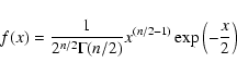$\begin{displaymath}f(x)=\frac{1}{2^{n/2}\Gamma(n/2)}x^{(n/2-1)}\exp\left(-\frac{x}{2}\right) \end{displaymath}$

(1)

where n is the d.o.f., and $\Gamma$ is the Gamma function. From this general formulation we can extract the probability density for u being the sum of the square of non-normalized random variables having a Gaussian distribution. This is done using a change of variable:

$\begin{displaymath}x=\frac{u}{s} \end{displaymath}$

(2)

where s is the rms value of the individual random variable making the distribution. The probability density is then written as

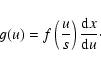$\begin{displaymath}g(u)=f\left(\frac{u}{s}\right) \frac{{\rm d}x}{{\rm d}u}\cdot \end{displaymath}$

(3)

Then we obtain the following probability density for u:

$\begin{displaymath}g(u)=\frac{1}{2^{n/2}\Gamma(n/2)}\frac{u^{(n/2-1)}}{s^{n/2}}\exp\left(-\frac{u}{2s}\right)\cdot \end{displaymath}$

(4)

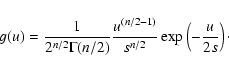
Since we deal not with individual Fourier components distributed as $\chi ^{2}$ with one d.o.f. but with a power spectrum, here we change parameter. We write:

S=2s

(5)

where S is the mean of the power spectrum that we usually utilize in the model of the $\chi ^{2}$ with 2 d.o.f. statistics. With this minor change we now have:

$\begin{displaymath}g(u)=\frac{1}{\Gamma(n/2)}\frac{u^{(n/2-1)}}{S^{n/2}}\exp\left(-\frac{u}{S}\right)\cdot \end{displaymath}$

(6)

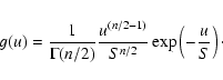
Finally, we change variable. What we observe is really u, i.e. the random variable associated with the sum of the power spectra (there are p=n/2 summed power spectra). By doing a simple normalization, we can greatly simplify the statistics:

$\begin{displaymath}v=\frac{u}{p} \end{displaymath}$

(7)

where v is the random variable associated with the observed spectrum u divided by the number of summed spectra p; when p=1, we get back the original power spectrum as only one spectrum is used. Then the probability density is written as:

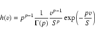$\begin{displaymath}h(v)=p^{p-1}\frac{1}{\Gamma(p)}\frac{v^{p-1}}{S^{p}}\exp\left(-\frac{p v}{S}\right) \end{displaymath}$

(8)

the associated pseudo log likelihood can be written as:

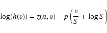$\begin{displaymath}\log(h(v))=z(n,v)-p\left(\frac{v}{S}+\log S\right) \end{displaymath}$

(9)

where z(n,v) is a function of v and n. When the minimization of the log likelihood l is performed on the data, we have:

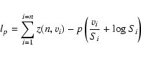$\begin{displaymath}l_{p}=\sum_{i=1}^{i=n} z(n,v_{i})-p\left(\frac{v_{i}}{S_{i}}+\log S_{i}\right) \end{displaymath}$

(10)

where v_i and S_i are respectively the data and the model at the ith bin; all bins are assumed independent. It is now clear that minimization of the likelihood for the mean of the sum of p power spectra is the same as minimizing the following function:

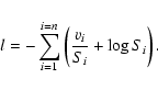$\begin{displaymath}l=-\sum_{i=1}^{i=n} \left(\frac{v_{i}}{S_{i}}+\log S_{i}\right). \end{displaymath}$

(11)

The terms in parentheses is the usual expression for a $\chi ^{2}$ with 2 d.o.f. When p=1, this is exactly what we minimize. The curvature of the minimized function providing the error bars is increased by p; this should be taken into account when computing the error bars (divide by $\sqrt{p}$ as it can be derived from Appourchaux et al. 1998).

3 Procedure for fitting the mean of the sum of p power spectra

Here we give a practical procedure for fitting the sum of p spectra using the regular MLE code used for spectra with a $\chi ^{2}$ with 2 d.o.f.:

compute the sum of the p power spectra;
divide the sum by p;
fit the model to the mean spectrum using the $\chi ^{2}$ with 2 d.o.f. statistics;
normalize error bars provided by the routines by dividing them by $\sqrt{p}$ .

There is no approximation performed here. The procedure only applies to independent power spectra having independent frequency bins.

4 Conclusions

This technique has been implemented by Jiménez et al. (2002) at the request of the author. It has been proven to be effective and should be used in helioseismology (or other fields) whenever deemed necessary.

Acknowledgements

Thanks to Frederic Baudin for suggesting the writing of this Research Note, and to Antonio Jiménez for triggering the scientific mind of a referee.

References