![[*]](/icons/foot_motif.gif)
A&A 412, 57-67 (2003)
DOI: 10.1051/0004-6361:20031412
G. Paturel1 - G. Theureau2,3 - L. Bottinelli2,4 - L. Gouguenheim 2,4 - N. Coudreau-Durand 2 - N. Hallet 2 - C. Petit1
1 - Observatoire de Lyon, avenue Charles-André, 69561 Saint-Genis Laval Cedex, France
2 -
LPCE, CNRS-Orléans, 3A avenue de la recherche scientifique, 45071 Orléans Cedex 02, France
3 -
Observatoire de Paris-Meudon, GEPI, 5 place Jules Janssen, 92195 Meudon Cedex, France
4 -
Université Paris-Sud, Bât. 470, 15 rue Georges Clémenceau, 91405 Orsay Cedex, France
Received 25 March 2003 / Accepted 29 July 2003
Abstract
After a compilation of HI data from 611 references and new observations made in Nançay,
we produce a catalog of homogenized HI data for 16781 galaxies.
The homogenization is made using the EPIDEMIC method from which
all data are progressively converted into the adopted standard.
The result is a catalog giving: 1) the logarithm of twice the maximum
rotation velocity,
 ,
converted to the system of Mathewson et al. (1996).
This quantity is given without correction for inclination;
2) the HI magnitude, m21, (area of the 21-cm line width expressed in magnitude)
converted to the flux system of Theureau et al. (1998); 3) the HI velocity,
,
converted to the system of Mathewson et al. (1996).
This quantity is given without correction for inclination;
2) the HI magnitude, m21, (area of the 21-cm line width expressed in magnitude)
converted to the flux system of Theureau et al. (1998); 3) the HI velocity,
 ,
expressed with the optical definition (i.e., using wavelengths instead frequencies).
The typical uncertainties are: 0.04 for
,
0.25 mag for m21and 9 km s-1 for
.
,
expressed with the optical definition (i.e., using wavelengths instead frequencies).
The typical uncertainties are: 0.04 for
,
0.25 mag for m21and 9 km s-1 for
.
Key words: galaxies: general - catalogs
The data are regularly maintained and the methods of homogenization are
regularly revisited in order to take into account the evolution of measurements.
In 1982 we collected HI measurements (21-cm line width, HI flux or
HI radial velocity) for 1210 galaxies (Bottinelli et al. 1982)
and for 6439 galaxies in 1990 (Bottinelli et al. 1990).
Today, we have measurements for 16 781 galaxies. This increase
could alone justify a new publication but another reason pushes us
to revisit the method of homogenization:
Many new measurements of logarithms of rotation velocity (hereafter,
),
obtained from rotation curves, are now available in the literature.
This gives us a new way to convert directly the observed 21-cm line widths
into the astrophysical parameter
.
Further, the velocity resolution has been considerably improved (in 1982, 32 percent of our catalogue had measurements with a poor resolution of 63.5 km s-1 and only 50 percent of the sample were obtained with a resolution better than 25 km s-1. In the present catalogue, 92 percent of the data are obtained with a resolution better than 25 km s-1 and only a few galaxies (46) have no resolution better than 50 km s-1. This means that the correction for instrumental effects can be made effectively using a simple linear approximation.
In Sect. 2 we give a description of the present compilation of HI data in which new observations are included. The new observations are presented in the appendix. In Sect. 3 we briefly review the method of analysis (the EPIDEMIC method) applied to this study. Then, in Sects. 4-6, we study the homogenization of 21-cm line widths, of HI radial velocities and of 21-cm line fluxes, respectively. This allows us to produce a catalog of mean homogenized HI data, presented in the final section.
These data, together with the whole catalogue, are now available through the HYPERLEDA database (leda.univ-lyon1.fr), a project which aims at extending the capabilities of LEDA.
We collected HI data from 611 papers. The full references with their code numbers are available in electronic form at the CDS. Further, for 809 galaxies we added new measurements made with the radiotelescope of Nançay. These new data are presented in the appendix.
This compilation provides us with 51 113 measurements of 21-cm line widths or maximum velocity rotation, 31 157 measurements of HI radial velocity and 25 764 measurements of HI flux (area of the 21-cm line) for 16 781 galaxies. These data are characterized by some secondary parameters: telescope, velocity resolution, definition of the 21-cm line width and bibliographic reference. Some additional parameters are also required: For instance the diameter and axis ratio of the observed galaxy (and sometimes the position angle) are needed to correct for the beam filling effect (see the section where the homogenization of fluxes is described). The optical radial velocity is also useful to provide a final check of velocities. These additional parameters are taken from LEDA.
Table 1 gives the list of telescopes with their code number and the number of 21-cm line widths obtained by each.
Table 1: List of telescopes. Column 1: number of published 21-cm line widths; Col. 2: code number of the telescope in LEDA; Col. 3: Name of the telescope.
![\begin{figure}
\par\resizebox{8.8cm}{!}{\includegraphics[clip]{ms3774_fig1.eps}}
\end{figure}](/articles/aa/full/2003/47/aa3774/img12.gif) |
Figure 1: Histogram of velocity resolutions. |
| Open with DEXTER | |
Figure 1 gives the histogram of velocity resolutions. These resolutions will be shared in four classes designated by r, where r represents the mean velocity resolution in km s-1(see Table 4):
 km s-1 (r=8 km s-1);
 km s-1 (r=16 km s-1);
 km s-1 (r=21 km s-1);
Table 2: Definition of the method of measurement of 21-cm line width. The columns are arranged as follows: Col. 1: number of published 21-cm line widths; Col. 2: code number of the method in LEDA; Col. 3: description of the method.
Finally, Table 3 presents the references giving more than 300 measurements. The reference numbers are arbitrary. They are internal numbers in LEDA. The full table, sorted by the number of entries, is available in electronic form at the CDS. It is also available sorted in alphabetic order.
Table 3:
List of the richest references (n>300). The columns are arranged as follows:
Col. 1: number of measurements of 21-cm line width or
;
Col. 2: code number of the reference in LEDA;
Col. 3: Full reference. The full table is available in electronic form at the CDS.
 ,
where
,
where  is the standard
deviation of a preliminary comparison and n the number of measurements.
References having no intersection with the standard sample during the preliminary
comparison are included following their population.
All inclusions are made using weighted means.
The standard sample receives the best standard deviation divided by
is the standard
deviation of a preliminary comparison and n the number of measurements.
References having no intersection with the standard sample during the preliminary
comparison are included following their population.
All inclusions are made using weighted means.
The standard sample receives the best standard deviation divided by  .
This
assumes that it has the same scatter as the second best sample.
.
This
assumes that it has the same scatter as the second best sample.
Obviously, the parameters used to make the classification must be relevant and we have to check that the equation of conversion is properly defined. Further, it is necessary to check that the conversion equation is reasonable (for instance, the conversion of flux should have a slope not very different from one in a log-log scale). Let us see now the application of this method to the homogenization of rotation velocities, heliocentric radial velocities and HI fluxes.
 .
It is important to note that in this paper, we consider always the quantity
,
that is twice the maximum rotation velocity in a logarithmic scale, in order to have a
definition comparable with the log of a 21-cm line width.
Note that
is not corrected for the inclination.
The physical parameter measuring the maximum velocity rotation
.
It is important to note that in this paper, we consider always the quantity
,
that is twice the maximum rotation velocity in a logarithmic scale, in order to have a
definition comparable with the log of a 21-cm line width.
Note that
is not corrected for the inclination.
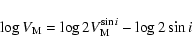
The physical parameter measuring the maximum velocity rotation  is then
related to
following the relation
is then
related to
following the relation
 |
(1) |
The raw 21-cm line widths are denoted  .
They must be corrected
for instrumental effects
(velocity resolution r, standardization of the level of measurement, l)
and then converted into
after correcting for internal velocity dispersion.
.
They must be corrected
for instrumental effects
(velocity resolution r, standardization of the level of measurement, l)
and then converted into
after correcting for internal velocity dispersion.
The adopted standard sample of
deduced from rotation curves is
the sample by Mathewson et al. (1996) because it is the largest homogeneous one.
Our new way of analysis allows us to convert directly
 into
because we now have a large enough standard sample of
.
The correction for the resolution, the conversion
to a standard level of measurement and the correction of internal dispersion are all done
in a single operation provided that the data are distributed into homogeneous
subsamples.
into
because we now have a large enough standard sample of
.
The correction for the resolution, the conversion
to a standard level of measurement and the correction of internal dispersion are all done
in a single operation provided that the data are distributed into homogeneous
subsamples.
The choice of a log-log conversion relation can be predicted in the case of good velocity resolution. However, we verified that it is linear. As an example, we show in Fig. 2 the relationship for the two richest subsamples.
It can be noted that some discrepant points are visible. They can result
from an HI confusion by a close galaxy present in the lobe of the
radiotelescope or from a bad detection. These discrepant
objects are recorded for each regression in order to put a question mark
on the final
value.
![\begin{figure}
\par\resizebox{8.8cm}{!}{\includegraphics[clip]{ms3774_fig2.eps}}
\end{figure}](/articles/aa/full/2003/47/aa3774/img25.gif) |
Figure 2:
An example of the regression used to convert log of 21-cm line widths
into
.
Both quantities are observed ones, uncorrected for inclination.
refers to measurements made with a same class of
velocity resolution and a same level of measurement.
The regression is quite linear.
The list of discrepant measurements (tiny dots) obtained with all
references will be used to correct (or to erase) doubtful measurements. |
| Open with DEXTER | |
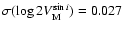
The total sample is divided into 26 subsamples defined by a given
resolution r and a given level l.
After the preliminary test, the standard deviation of the initial standard
sample of
is taken as
 .
The results of the EPIDEMIC method is shown in Table 4.
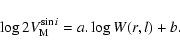
This table gives the slope a and the intercept b of the equation:
.
The results of the EPIDEMIC method is shown in Table 4.
This table gives the slope a and the intercept b of the equation:
 |
(2) |
,
the number of points n of the regression, and  ,
the growing number of standard measurements.
,
the growing number of standard measurements.
This table gives the coefficients to convert any 21-cm line width (measured
with a resolution r at a level l) into
.
It gives also
the standard deviation
assigning a weight
 to the measurement.
It is visible from Table 4 that the level l=5 (50% of the maximum) gives a slope close to one, while the level l=1 (20% of the maximum) gives a slope significantly larger. One can see also that the low-resolution class (r=41 km s-1), for l=1 or l=5, gives systematically larger standard deviations. This reflects the fact that this class is less accurate and less homogeneous.
Table 4:
Correction of
to
.
This table gives
the conversion coefficients and the mean error
for the 26 subsamples (level and resolution). l is the level code (see Table 2). r is the mean velocity resolution in km s-1.
The full table is available in the electronic version of the journal.
As a refinement
we apply again the EPIDEMIC method using the bibliographic references
to define the different homogeneous classes. The
measurements by
Mathewson et al. (1996) are used as a standard. For this application, the
are first converted to
using the previous result (Table 4).
This will allow us to improve the results for some references.
If the first correction was perfect, the new slope should be a=1 and the zero-point
should be b=0 for any references. We keep only those references for which the slope
or the zero point are significantly different from that. A Student's t-test
is first made on the slope a. If the slope is not significantly different from 1 at the
0.01 probability level, it is taken as 1, exactly, and b is recalculated. Another
t-test is made on the new b value. If it does not differ significantly from zero the
reference does not need additional correction. Otherwise, the values of a or b are adopted, as given in Table 5.
65 references needed an additional correction.
We established a list of 2087 galaxies that may have
one discrepant measurement. This list will be used when we construct the final
homogeneous catalog.
Table 5:
Correction of
to the adopted standard (ref. 23286). This
table gives the conversion coefficients and the mean error
for the 65 references requiring an additional correction.
The full table is available in the electronic version of the journal.
Before applying the EPIDEMIC method, these magnitudes must be corrected
for the beam filling effect.
Sometimes radioastronomers publish corrected fluxes but, when possible,
we prefer to collect raw fluxes in order to have a homogeneous conversion.
The form of the correction is well established.
We will use the correction established in our previous study (Bottinelli et al. 1990).
Let us recall how the corrected HI magnitude, m21c, is calculated:
 |
(5) |
 |
(6) |
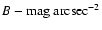 and
and  is the half power beam size of the considered
radiotelescope. In this equation D25, d25 and
are expressed
with the same unit (i.e. arcmin). The parameter x is
is the half power beam size of the considered
radiotelescope. In this equation D25, d25 and
are expressed
with the same unit (i.e. arcmin). The parameter x is
 (Bottinelli et al. 1990). We will keep this value.
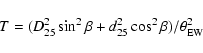
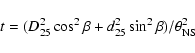
For the Nançay radiotelescope the correction is more complex because the half
power beam is not circular ( 21'NS
21'NS  4'EW). We adopted the
the same correction (Rel. (4)) but:
4'EW). We adopted the
the same correction (Rel. (4)) but:
 |
(7) |
 |
(8) |
 is the position angle of the considered galaxy (counted from North
towards East) and where the ellipse of the half power bean size is defined by
is the position angle of the considered galaxy (counted from North
towards East) and where the ellipse of the half power bean size is defined by
 and
and
 .
D25, d25 and
are calculated following
Paturel et al. (2003, Paper I).
.
D25, d25 and
are calculated following
Paturel et al. (2003, Paper I).
The EPIDEMIC method can now be applied to m21c. We expect a systematic
effect depending on the radiotelescope itself. Thus, the classification of
the EPIDEMIC method is built using the code for each radiotelescope. We use
the Nançay radiotelescope (t=1) as a standard because its large
beam is less sensitive to the beam filling effect
and because it constitutes one of the largest sample (see Table 1).
The adopted equation of conversion is:
| m21 c(t=1) = m21 c (t) + b. | (9) |
Table 6:
Correction of m21 to the scale of Nançay. This table gives
the the zero-point shift and the mean error
for the different radiotelescope (Col. 1). By its adoption as a standard, the Nançay
radiotelescope (t=1) has b=0 and its standard deviation is
 .
The full table is available in the electronic version of the journal.
.
The full table is available in the electronic version of the journal.
We check reference by reference to find specific corrections of
the zero-point of the m21c magnitudes. They are first converted to the
Nançay scale using the results from
Table 6. For this second run, we adopted as a standard
the reference 23289. Nevertheless, in order to reduce the number of references
requiring a specific correction, it has been shifted by 0.2 mag (this correction
has been obtained from a weighted mean of individual shifts, reference by reference).
In other words, the actual zero-point of the magnitude scale is built from a mean system.
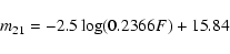
The final m21F magnitudes is then given by:
| m21 F = m21 c (t=1) + br - 0.2. | (10) |
Table 7: Correction of m21 to the standard (ref. 23289). This table gives the zero-point shift and its mean error for the 46 references requiring an additional correction. The full table is available in the electronic version of the journal.
The EPIDEMIC method is now used for the heliocentric radial velocities.
Note that all these velocities should be expressed with the optical
convention
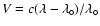 .
We do not expect any sources of systematic effects. Thus we simply
check that there is no reference effect. The homogeneous classes of the
EPIDEMIC method are thus made using the reference code. The standard
sample is the reference 23289 because it is the largest one.
Two references (23000 and 23316) show a significant effect. It appears
that they are expressed as
.
We do not expect any sources of systematic effects. Thus we simply
check that there is no reference effect. The homogeneous classes of the
EPIDEMIC method are thus made using the reference code. The standard
sample is the reference 23289 because it is the largest one.
Two references (23000 and 23316) show a significant effect. It appears
that they are expressed as
 ,
where
,
where  is the frequency. This effect disappears for these references when we applied the correction
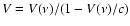 .
One reference (23286) showed a barely significant departure
from the standard. It could have been corrected by applying a scaling factor
.
One reference (23286) showed a barely significant departure
from the standard. It could have been corrected by applying a scaling factor
 .
Because reference 23286 was adopted as the standard for rotation
velocity measured from rotation curves, one can ask if this effect could
affect the accuracy of
.
One can calculate that
this effect is at least 40 times smaller than the typical uncertainty and is
completely negligible.
.
Because reference 23286 was adopted as the standard for rotation
velocity measured from rotation curves, one can ask if this effect could
affect the accuracy of
.
One can calculate that
this effect is at least 40 times smaller than the typical uncertainty and is
completely negligible.
Finally, we have to estimate the standard deviation for each reference.
As we did in our previous compilations, the best way consists of
finding a correlation between the standard deviation and the resolution
velocity. For this purpose, we apply the EPIDEMIC method using the true
velocity resolution R as a parameter of classification. For each regression
we get the standard deviation and we plot it as a function of the
resolution. The result is shown in Fig. 3. A direct
regression leads to the relation:
 .
This result is
compatible with the result we obtained earlier (Bottinelli et al. 1990):
.
This result is
compatible with the result we obtained earlier (Bottinelli et al. 1990):
 .
Nevertheless, we prefer to calculate the
regression using only the resolution smaller than 24 km s-1 because
the sample is dominated by small resolutions (see Fig. 1).
The result is thus
.
Nevertheless, we prefer to calculate the
regression using only the resolution smaller than 24 km s-1 because
the sample is dominated by small resolutions (see Fig. 1).
The result is thus
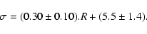 |
(11) |
for large resolutions, i.e., to reduce
the weight of old, poor resolution measurements.
This justifies also that we adopted this last solution.
In Fig. 3 this solution is drawn.
![\begin{figure}
\par\resizebox{8.8cm}{!}{\includegraphics[clip]{ms3774_fig3.eps}}
\end{figure}](/articles/aa/full/2003/47/aa3774/img75.gif) |
Figure 3:
Empirical relation between the velocity resolution r and the standard deviation
of the regressions V(r) vs. V(
 ).
The adopted solution calculated with
the resolution smaller than 24 km s-1 is represented by the full line. ).
The adopted solution calculated with
the resolution smaller than 24 km s-1 is represented by the full line. |
| Open with DEXTER | |
We established a list of 710 galaxies that may have one discrepant velocity to be noted in the final homogeneous catalog.
As an additional test, we checked the homogenized HI velocities against
the optical ones extracted from the LEDA database. The direct regression
leads to the following result (obtained with 10 019 galaxies):
 |
(12) |
 km s-1 and the mean difference
of both systems (
km s-1 and the mean difference
of both systems (
 km s-1) has no practical incidence.
This comparison provided us with another list of 634 galaxies for which
there is a discrepancy between optical and HI velocities.
km s-1) has no practical incidence.
This comparison provided us with another list of 634 galaxies for which
there is a discrepancy between optical and HI velocities.
Using the results of the previous sections we produced a catalog of
homogenized HI data for 16 781 galaxies.
The distribution of heliocentric radial velocities (Fig. 4)
shows a bump around 5000 km s-1, although the completeness in volume
is satisfied only up to 2000 km s-1.
This corresponds to the nearest clusters surrounding the Local Super Cluster.
![\begin{figure}
\par\resizebox{8.8cm}{!}{\includegraphics[clip]{ms3774_fig4.eps}}
\end{figure}](/articles/aa/full/2003/47/aa3774/img79.gif) |
Figure 4: Distribution of heliocentric radial velocities. |
| Open with DEXTER | |
Let us recall briefly how the homogenized data are calculated.
The 21-cm line widths are first converted into
using
empirical linear relations (Table 4) depending on the velocity
resolution and on the level of measurement. For some references
an additional correction is applied (Table 5).
The mean error of each individual measurement comes from the
standard deviation of the linear regression used for the
last conversion (Tables 4 or 5).
The HI magnitudes m21 are first corrected for the beam filling
effect (Rel. (4)) and then converted to the Nançay
scale using linear relations (Table 6) depending on the
radiotelescope used. For some references an additional correction
is applied (Table 7).
The mean error of each individual measurement is also calculated
as previously stated (Tables 6 or 7).
The HI heliocentric radial velocities are not transformed (except
one reference that is transformed into the optical definition and
one that is corrected for a small scale effect).
The mean error of each measurement is calculated as a funtion
of the velocity resolution. For unknown velocity resolution we
adopted a mean standard deviation of 15 km s-1.
Finaly, for each galaxy the weighted mean and its actual error are calculated.
This actual error (Paturel et al. 1997) takes into account the
accuracy of each individual source of data and the dispersion
of the considered measurements. It gives a realistic description of the uncertainty
attached to each mean value. Note that some data receive a flag (:) to show that they may include a discrepant measurement.
As far as possible, discordant measurements are rejected
(typically when there are several measurements in agreement and one
discordant).
In order to show the quality of the data the histograms of actual
errors on
,
m21 and
 are given in Fig. 5.
The beginning of the final catalog is given
in Table 8. This catalog is available in electronic form at the CDS.
are given in Fig. 5.
The beginning of the final catalog is given
in Table 8. This catalog is available in electronic form at the CDS.
![\begin{figure}
\par\resizebox{8.8cm}{!}{\includegraphics[clip]{ms3774_fig5a.eps}...
...}\par\resizebox{8.8cm}{!}{\includegraphics[clip]{ms3774_fig5c.eps}}
\end{figure}](/articles/aa/full/2003/47/aa3774/img80.gif) |
Figure 5:
Distribution of mean errors on
,
m21and
. |
| Open with DEXTER | |
Table 8:
The final catalog of homogenized HI data. The catalog gives these data
for 16 781 galaxies. The full catalog is available in electronic form at the CDS.
Col. 1: PGC number from LEDA;
Col. 2: Alternate name from LEDA;
Col. 3: Right Ascension and Declination for the equinox 2000, in hours, minutes, seconds
and tenths, and degrees, arcminutes and arcseconds;
Col. 4: Mean homogenized decimal logarithm of twice the maximum rotation velocity uncorrected
for inclination (
in km s-1);
Col. 5: Mean homogenized 21-cm magnitude (see Eq. (3));
Col. 6: Mean homogenized HI heliocentric radial velocity (in km s-1);
Each parameter is given with a flag f telling if it is uncertain (f=1).
Acknowledgements
We thank R. Garnier for helping us in the selection of references and the observers of the Nançay radiotelescope for their contribution to the observations. We thank Dr. J. J. Gallagher III for very useful comments on the manuscript.
Table A.1: New observations. (The full table is available in electronic form at the CDS). Col. 1: PGC number from LEDA; Col. 2: Alternate name from LEDA; Col. 3: Right Ascension and Declination for the equinox 2000, in hours, minutes, seconds and tenths, and degrees, arcminutes and arcseconds; Col. 4: 21-cm line width at 20% of the maximum (in km s-1); Col. 5: 21-cm line width at 50% of the maximum (in km s-1); Col. 6: HI heliocentric radial velocity (in km.s-1); Col. 7: HI flux (area of the 21-cm line) (in mJy km s-1); Col. 8: Signal to Noise ration; Col. 9: Quality of the line (see text) and notes (see Table A.3).
In this section we present the HI follow-up of a set of galaxies selected in the infrared (IRAS) and near-infrared (DENIS) with the aim of starting to build of a TF catalogue in BIJHK bands. This survey is the preliminary step of the present cosmological key-project of the refurbished Nançay radiotelescope, KLUN+, which intends to collect new HI profiles of some 8000 galaxies in the period 2001-2005, on the basis of a DENIS and 2-MASS target selection.
Objects have been selected according to their IRAS flux,
S60> 0.6 Jy,
and/or their I magnitude, I < 14.5. Radial velocities where known
except for some galaxies at low galactic latitude (211 objects with
 ).
).
The present catalogue contains the HI profile and parameters (velocity measurements, 21-cm line widths, HI fluxes, signal to noise ratio, and rms noise) for 817 spiral galaxies.
All these observations have been carried out between 1994 and 1998
with the old system of the meridian-transit Nançay radiotelescope (France).
This instrument is a single dish antenna with a collecting area of 6912 m2equivalent to that of a 94 m-diameter parabolic dish.
The half-power beam width at 21-cm is 3.6 arcmin (EW) 22 arcmin
(NS) (at zero declination). Observations where limited to declination
 .
.
The minimal system temperature at
 was about 37 K in both
horizontal and vertical polarizations.
The spectrometer was a 1024-channel autocorrelator of 6.4 MHz bandwidth. The
spacing of the channels corresponds to 2.6 km s-1 at 21 cm with
a bank of 512 channels in each polarization. After boxcar smoothing the
final resolution is typically 10 km s-1. In the velocity-search mode
the 1024 channels are split in four banks of 256 channels leading to a
range of 4800 km s-1 (generally from 400 to 5200 km s-1 or from 5200 to 10 000 km s-1).
The gain of the antenna has been calibrated according to Fouqué et al. (1990).
was about 37 K in both
horizontal and vertical polarizations.
The spectrometer was a 1024-channel autocorrelator of 6.4 MHz bandwidth. The
spacing of the channels corresponds to 2.6 km s-1 at 21 cm with
a bank of 512 channels in each polarization. After boxcar smoothing the
final resolution is typically 10 km s-1. In the velocity-search mode
the 1024 channels are split in four banks of 256 channels leading to a
range of 4800 km s-1 (generally from 400 to 5200 km s-1 or from 5200 to 10 000 km s-1).
The gain of the antenna has been calibrated according to Fouqué et al. (1990).
Table A.2:
Periods of gain stability and correction factors (
 ).
).
![\begin{figure}
\par\resizebox{17cm}{!}{\includegraphics[clip]{ms3774_figA1.eps}}
\end{figure}](/articles/aa/full/2003/47/aa3774/img86.gif) |
Figure A.1: Sample of the 21-cm line profiles. The full figure is availaible in the electronic version at http://www.edpsciences.org |
Table A.3: Comments on some galaxies. The full table is available in electronic form at the CDS. The references concerning these comments are given at the end of the table.
We used the Nançay processing package SIR (Système Interactif de Réduction). The processing chain consist of a selection of good observation cycles (one "observation'' is a series of on/off observational sequences), the straightening of the base-line by a polynomial fit, and the application of a boxcar smoothing. The maximum of the line is determined by eye as the mean value of the maxima of each profile's horn after taking into account the medium noise (evaluated in the base-line). The widths, measured at the standard levels 20% and 50% of that maximum, correspond to the "distance'' separating the two external points of the profile at these intensity levels.
Together with some other large HI surveys in Nançay, all the data are presented in the on-line Nançay HI extragalactic database (http://klun.obs-nancay.fr). The observed radial velocities are listed in Table A.1 (Col. 6) and correspond to the median point of the 21-cm line profile measured at 20% of maximum intensity and translated into the optical velocity scale. The average uncertainty on V20 is about 8 km s-1 and does not exceed 20 km s-1.
The widths W20 and W50 are expressed in km s-1 (Table A.1, Cols. 4 and 5) and correspond to direct measurements on the 21-cm profiles.
HI-fluxes
 (Table A.1, Col. 7) are expressed in Jy km s-1 and
calibrated using as a reference a set of 9 calibrators regularly
observed during the survey period (see Theureau et al. 1998).
The evolution of the ratio
(Table A.1, Col. 7) are expressed in Jy km s-1 and
calibrated using as a reference a set of 9 calibrators regularly
observed during the survey period (see Theureau et al. 1998).
The evolution of the ratio
 with time allows us to supervise the Nançay system and to get
for each observation the optimal flux measurement. In total, six periods of gain
stability have been considered, with corresponding flux correction factors (see Table A.2).
From this table and the number of ON/OFF integration cycles observed in each period for
a given object, we have been able to correct the flux measurement for each galaxy.
Each measurement has been corrected for the Nançay beam effect when position angle,
diameter and axis ratio were known (beam-uncorrected flux are flagged with a star).
with time allows us to supervise the Nançay system and to get
for each observation the optimal flux measurement. In total, six periods of gain
stability have been considered, with corresponding flux correction factors (see Table A.2).
From this table and the number of ON/OFF integration cycles observed in each period for
a given object, we have been able to correct the flux measurement for each galaxy.
Each measurement has been corrected for the Nançay beam effect when position angle,
diameter and axis ratio were known (beam-uncorrected flux are flagged with a star).
HI profiles have been classified in four classes according to their quality:
Table 4:
Correction of
to
 .
This table gives
the conversion coefficients and the mean error
for the 26 subsamples (level and resolution). l is the level code (see Table 2). r is the mean velocity resolution in km s-1.
.
This table gives
the conversion coefficients and the mean error
for the 26 subsamples (level and resolution). l is the level code (see Table 2). r is the mean velocity resolution in km s-1.
Table 5:
Correction of
to the adopted standard (ref. 23286). This
table gives the conversion coefficients and the mean error
for the 65 references requiring an additional correction.
Table 6:
Correction of m21 to the scale of Nançay. This table gives
the the zero-point shift and the mean error
for the different radiotelescope (Col. 1). By its adoption as a standard, the Nançay
radiotelescope (t=1) has b=0 and its standard deviation is
.
Table 7: Correction of m21 to the standard (ref. 23289). This table gives the zero-point shift and its mean error for the 46 references requiring an additional correction.
![\begin{displaymath}m_{21}^c = m_{21} -1.25 \log [(1+xT)(1+xt)]
\end{displaymath}](/articles/aa/full/2003/47/aa3774/img48.gif)
![\begin{figure}\par\includegraphics[width=17cm,clip]{page01.eps}
\end{figure}](/articles/aa/full/2003/47/aa3774/img290.gif)
![\begin{figure}\par\includegraphics[width=17cm,clip]{page02.eps}
\end{figure}](/articles/aa/full/2003/47/aa3774/img291.gif)
![\begin{figure}\par\includegraphics[width=17cm,clip]{page03.eps}
\end{figure}](/articles/aa/full/2003/47/aa3774/img292.gif)
![\begin{figure}\par\includegraphics[width=17cm,clip]{page04.eps}
\end{figure}](/articles/aa/full/2003/47/aa3774/img293.gif)
![\begin{figure}\par\includegraphics[width=17cm,clip]{page05.eps}
\end{figure}](/articles/aa/full/2003/47/aa3774/img294.gif)
![\begin{figure}\par\includegraphics[width=17cm,clip]{page06.eps}
\end{figure}](/articles/aa/full/2003/47/aa3774/img295.gif)
![\begin{figure}\par\includegraphics[width=17cm,clip]{page07.eps}
\end{figure}](/articles/aa/full/2003/47/aa3774/img296.gif)
![\begin{figure}\par\includegraphics[width=17cm,clip]{page08.eps}
\end{figure}](/articles/aa/full/2003/47/aa3774/img297.gif)
![\begin{figure}\par\includegraphics[width=17cm,clip]{page09.eps}
\end{figure}](/articles/aa/full/2003/47/aa3774/img298.gif)
![\begin{figure}\par\includegraphics[width=17cm,clip]{page10.eps}
\end{figure}](/articles/aa/full/2003/47/aa3774/img299.gif)
![\begin{figure}\par\includegraphics[width=17cm,clip]{page11.eps}
\end{figure}](/articles/aa/full/2003/47/aa3774/img300.gif)
![\begin{figure}\par\includegraphics[width=17cm,clip]{page12.eps}
\end{figure}](/articles/aa/full/2003/47/aa3774/img301.gif)
![\begin{figure}\par\includegraphics[width=17cm,clip]{page13.eps}
\end{figure}](/articles/aa/full/2003/47/aa3774/img302.gif)
![\begin{figure}\par\includegraphics[width=17cm,clip]{page14.eps}
\end{figure}](/articles/aa/full/2003/47/aa3774/img303.gif)
![\begin{figure}\par\includegraphics[width=17cm,clip]{page15.eps}
\end{figure}](/articles/aa/full/2003/47/aa3774/img304.gif)
![\begin{figure}\par\includegraphics[width=17cm,clip]{page16.eps}
\end{figure}](/articles/aa/full/2003/47/aa3774/img305.gif)
![\begin{figure}\par\includegraphics[width=17cm,clip]{page17.eps}
\end{figure}](/articles/aa/full/2003/47/aa3774/img306.gif)
![\begin{figure}\par\includegraphics[width=17cm,clip]{page18.eps}
\end{figure}](/articles/aa/full/2003/47/aa3774/img307.gif)
![\begin{figure}\par\includegraphics[width=17cm,clip]{page19.eps}
\end{figure}](/articles/aa/full/2003/47/aa3774/img308.gif)
![\begin{figure}\par\includegraphics[width=17cm,clip]{page20.eps}
\end{figure}](/articles/aa/full/2003/47/aa3774/img309.gif)
![\begin{figure}\par\includegraphics[width=17cm,clip]{page21.eps}
\end{figure}](/articles/aa/full/2003/47/aa3774/img310.gif)
![\begin{figure}\par\includegraphics[width=17cm,clip]{page22.eps}
\end{figure}](/articles/aa/full/2003/47/aa3774/img311.gif)
![\begin{figure}\par\includegraphics[width=17cm,clip]{page23.eps}
\end{figure}](/articles/aa/full/2003/47/aa3774/img312.gif)
![\begin{figure}\par\includegraphics[width=17cm,clip]{page24.eps}
\end{figure}](/articles/aa/full/2003/47/aa3774/img313.gif)
![\begin{figure}\par\includegraphics[width=17cm,clip]{page25.eps}
\end{figure}](/articles/aa/full/2003/47/aa3774/img314.gif)
![\begin{figure}\par\includegraphics[width=17cm,clip]{page26.eps}
\end{figure}](/articles/aa/full/2003/47/aa3774/img315.gif)