D. A. N. Müller1 - V. H. Hansteen2 - H. Peter1
1 - Kiepenheuer-Institut für Sonnenphysik, Schöneckstr. 6, 79104 Freiburg, Germany
2 - Institute of Theoretical Astrophysics, University of Oslo, PO Box 1029, Blindern 0315, Oslo, Norway
Received 18 June 2003 / Accepted 22 August 2003
Abstract
We report numerical calculations of the condensation of plasma in short
coronal loops, which have several interesting physical consequences.
Firstly, we propose a connection between small, cool loops (T < 106 K), which constitute one of the basic components of the solar transition region, and prominences, in
the sense that the same physical mechanism governs their dynamics:
Namely the onset of instability and runaway cooling due to strong
radiative losses. Secondly, we show that the temporal evolution of these
loop models exhibits a cyclic pattern of chromospheric evaporation,
condensation, motion of the condensation region to either side of the
loop, and finally loop reheating with a period of 4000-8000 s for a
loop of 10 Mm length. Thirdly, we have synthesized transition region
lines from these calculations which show strong periodic intensity
variations, making condensation in loops a candidate to account for
observed transient brightenings of solar transition region lines.
Remarkably, all these dynamic processes take place for a heating function which is
constant in time and has a simple exponential height dependence.
Key words: Sun: corona - Sun: transition region - Sun: UV radiation
Since Skylab, loops have been recognized as a vital ingredient in coronal structure and coronal energetics. Indeed, one could imagine that the corona is entirely composed of nested loops with varying lengths, temperatures, heating rates, and activity levels. A nested structure of low-lying cool loops was suggested by Dowdy et al. (1986) to explain the temperature dependence of the emission measure. Thus, building an understanding of loop energetics is obviously a desirable objective. There are alternative scenarios for the structure of the transition region (see, e.g., Mariska 1992). As recent SOHO/SUMER results have shown, however, small cool loops to constitute one of the basic building blocks of the transition region (Feldman et al. 2000), this paper will concentrate on the dynamics and energetics of cool loops.
The main components in the energy balance of static loops were identified by Rosner et al. (1978): They consist of the unknown heating, thermal conduction and radiative losses in the loop itself and at the transition region/chromosphere boundary. Roughly speaking one can understand static loop behavior quite well by assuming that the heat deposited by the heating mechanism in the corona is largely conducted back towards the chromosphere where it is radiated away. Due to the strong temperature dependence of the thermal conduction coefficient, this scenario almost invariably leads to apex loop temperatures of roughly 1 MK bounded by a geometrically small transition region as the temperatures fall towards 104 K and chromospheric densities at the loop footpoints. Variations in the heating rate are dealt with in this type of loop by chromospheric evaporation or coronal condensation such that the radiative losses at the top of the chromosphere balance the thermal conductive flux from above (Hansteen 1993). This behavior is almost independent of the details of the heat deposition - as long as radiative losses near the loop apex are not an important factor in the energy budget.
Clear as the model above seems, serious difficulties are encountered as soon as loop model predictions are confronted with the observations themselves. These difficulties are various and sundry (Mariska 1992) but might be summarized as follows: The differential emission measures predicted by the models gives a much lower line emission from the lower transition region, below 105 K, than what is observed (alternatively one could say that the line emission from the upper transition region, above 105 K, is predicted much too high). In addition it is very difficult to account for the pervasive average red shift of up to 10 km s-1 seen in lower transition region lines and blue-shifts in the upper transition region and low corona (Peter & Judge 1999).
Several proposals have been put forward to answer the difficulties outlined above. Dowdy et al. (1986) suggested a two-component transition region, consisting of magnetic funnels and a nested structure of low-lying, cool coronal loops. This new class of static loop solutions had been discussed by Antiochos & Noci (1986). Cally & Robb (1991) argued, however, that these cool loop solutions were unstable, and Cally (1990) proposed turbulent thermal conduction as an alternative hypothesis to explain the enhanced transition region emission. As for the spectral diagnostics of transition region lines, loop dynamics due to downward-propagating magneto-acoustic waves were shown to be a candidate to account for the pervasive redshifts (Hansteen 1993).
However, it was first with the observations by the SOHO and TRACE instruments that the importance of cool loops and loop dynamics has belatedly come to the foreground. Peter (2000) gives evidence for a multi-component structure of the transition region, and Feldman et al. (2001) reach the conclusion that regions of hotter and cooler plasma in the solar atmosphere are essentially disconnected from each other.
The question that is raised is what implications these new ideas have on our understanding of the structure and energetics of both cool and hot coronal loops. Obviously a time-dependent heating will produce a number of dynamic phenomena such as waves or material motions through evaporation or condensations. But as we will show below it is also found that within a certain parameter range of static mechanical energy deposition quite violent dynamics can ensue.
Numerous mechanisms of coronal heating have been proposed (e.g. wave
heating, nanoflares, magnetic reconnection), but independent of the
detailed process of energy release there is now observational evidence
that coronal loops are predominantly heated at the footpoints
(Aschwanden et al. 2001,2000). With heating
concentrated near the loop footpoints it is no longer certain that
sufficient energy to counter radiative losses is deposited near the loop
apex. In fact, for such loops static solutions with a hot midpoint may
no longer exist as the radiative loss rate increases strongly in the
loop center when the temperature decreases towards
![]() K.
If the magnetic field topology is such that the loop has a dip in the center,
footpoint heating can lead to the
condensation of plasma in the loop center and hence give rise to
prominence formation (Antiochos et al. 1999). It was also found by
Antiochos et al. (2000) that this type of prominence formation shows
a cycle of formation, motion, and destruction. Recently, it was
demonstrated by Karpen et al. (2001) that the condition of a
"dipped'' geometry is indeed not a necessary condition for prominence
formation in long loops (their work describes a loop of 340 Mm length).
A key element in their prominence scenario is the large ratio of loop
length to the damping length of the heating function, and the authors
argue that shorter loops with a smaller ratio should therefore behave
differently.
K.
If the magnetic field topology is such that the loop has a dip in the center,
footpoint heating can lead to the
condensation of plasma in the loop center and hence give rise to
prominence formation (Antiochos et al. 1999). It was also found by
Antiochos et al. (2000) that this type of prominence formation shows
a cycle of formation, motion, and destruction. Recently, it was
demonstrated by Karpen et al. (2001) that the condition of a
"dipped'' geometry is indeed not a necessary condition for prominence
formation in long loops (their work describes a loop of 340 Mm length).
A key element in their prominence scenario is the large ratio of loop
length to the damping length of the heating function, and the authors
argue that shorter loops with a smaller ratio should therefore behave
differently.
We present numerical calculations which show that, depending on the damping length of the heating function, condensation is also possible in short, cool coronal loops. We study the evolution of these loops, discuss static as well as dynamic solutions and finally calculate the time-dependent emission of transition region lines arising from this model.
We numerically solve the time-dependent hydrodynamic equations for conservation of mass, momentum and energy in one spatial dimension, coupled with the ionization rate equations for several elements and self-consistent radiative losses (cf. Hansteen 1993, for details). The modeled plasma is subjected to gravitational acceleration equal to that found on the solar surface. Thermal conduction, radiative losses and a coronal heating term are included in the energy equation.
The equations for mass conservation, momentum, energy, and ionization and recombination rates read as follows:
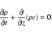 |
(1) |
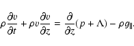 |
(2) |
 |
(3) |
![\begin{displaymath}%
\frac{\partial n_{ij}}{\partial t} + \frac{\partial}{\parti...
...n_{ij}(C_{ij}+\alpha_{ij}) \\
+ n_{ij+1}\alpha_{ij+1}\bigr].
\end{displaymath}](/articles/aa/full/2003/46/aah4613/img20.gif) |
(4) |
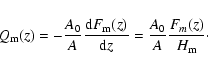
Here v denotes the velocity along the curvilinear loop coordinate, z, ![]() the component of the gravitational acceleration that is parallel to the magnetic field,
the component of the gravitational acceleration that is parallel to the magnetic field, ![]() the mechanical heating rate,
the mechanical heating rate,
![]() the radiative loss rate per unit volume, and
the radiative loss rate per unit volume, and ![]() a small "opacity heating'' term that is included in order to maintain chromospheric temperatures at roughly 7000 K.
The internal energy, e, is calculated as the sum of the thermal and internal energy including only ionization states, the contribution from the excitation energy is negligible.
The population of the ionization state j of element i is denoted by nij, while ionization rates and recombination rates are represented by Cij and
a small "opacity heating'' term that is included in order to maintain chromospheric temperatures at roughly 7000 K.
The internal energy, e, is calculated as the sum of the thermal and internal energy including only ionization states, the contribution from the excitation energy is negligible.
The population of the ionization state j of element i is denoted by nij, while ionization rates and recombination rates are represented by Cij and
![]() ,
respectively.
The artificial viscosity term
,
respectively.
The artificial viscosity term
![]() (according to von Neumann & Richtmyer 1950) is discussed by Hansteen (1993).
The thermal conduction is set to
(according to von Neumann & Richtmyer 1950) is discussed by Hansteen (1993).
The thermal conduction is set to
![]() (Spitzer 1962) with
(Spitzer 1962) with
![]() W m-1 s-1 K-7/2.
W m-1 s-1 K-7/2.
Radiative losses are computed assuming that the plasma is effectively
thin. While, ideally, one should solve the equation of radiative
transport in order to calculate the radiative losses, comparisons with
models where this has been done (Kuin & Poland 1991; Carlsson 2003) indicate that the errors incurred by
assuming effectively
thin losses in the
![]() line are not
significant to the energetics of the system in the upper chromosphere
and above. Radiative losses are due to collisional excitation of the
various ions comprising the plasma. We have included the elements
hydrogen, helium, carbon, oxygen, neon, and iron in the
radiative losses, as well as thermal bremsstrahlung, using the ionization and recombination rates given by
Arnaud & Rothenflug (1985) and Shull & van Steenberg (1982) and the collisional
excitation rates found through the HAO-DIAPER atomic data package
(Judge & Meisner 1994). The collisional excitation rate from the
ground state of hydrogen to its first excited state is computed from
coefficients found in Janev et al. (1987). Some of the
metals are treated by assuming ionization equilibrium and then deriving
an a priori radiative loss curve as a function of electron
temperature. On the other hand radiative losses from the ions
specifically mentioned in this study, i.e. losses from hydrogen, helium,
carbon and oxygen, are computed consistently with full time-dependent
rate equations.
line are not
significant to the energetics of the system in the upper chromosphere
and above. Radiative losses are due to collisional excitation of the
various ions comprising the plasma. We have included the elements
hydrogen, helium, carbon, oxygen, neon, and iron in the
radiative losses, as well as thermal bremsstrahlung, using the ionization and recombination rates given by
Arnaud & Rothenflug (1985) and Shull & van Steenberg (1982) and the collisional
excitation rates found through the HAO-DIAPER atomic data package
(Judge & Meisner 1994). The collisional excitation rate from the
ground state of hydrogen to its first excited state is computed from
coefficients found in Janev et al. (1987). Some of the
metals are treated by assuming ionization equilibrium and then deriving
an a priori radiative loss curve as a function of electron
temperature. On the other hand radiative losses from the ions
specifically mentioned in this study, i.e. losses from hydrogen, helium,
carbon and oxygen, are computed consistently with full time-dependent
rate equations.
The equations are formulated on a staggered, adaptive grid using the Reynolds transport theorem as described by Winkler et al. (1984) and the adaptive grid formulation suggested by Dorfi & Drury (1987). Particle and momentum fluxes are calculated according to the second-order upwind method of Van Leer (1974). This results in a set of equations which are solved implicitly by means of the Newton-Raphson scheme to advance the equations in time.
In order to parametrize the energy input into
the coronal loop, we specify the energy flux amplitude at the footpoints
of the loop,
![]() ,
and assume a mechanical heat flux that is
constant up to a height z1 and then decreases for
,
and assume a mechanical heat flux that is
constant up to a height z1 and then decreases for ![]() as
as
| (5) |
We will vary ![]() between 0.25 and 3.25 Mm in the models presented below.
For the mechanical energy flux we adopt the value of
between 0.25 and 3.25 Mm in the models presented below.
For the mechanical energy flux we adopt the value of
![]() W m-2 (the same as the one used by Hansteen & Leer 1995), and set z1 =1.75 Mm for a loop of 10 Mm length.
W m-2 (the same as the one used by Hansteen & Leer 1995), and set z1 =1.75 Mm for a loop of 10 Mm length.
The heating rate, i.e. the energy deposition per unit time and unit
volume, is given by the divergence of the energy flux:
Our model coronal loop has a total length of
10 Mm, consisting of a semicircular arch of 8 Mm length and a vertical
stretch of 1 Mm length at both ends. In Fig. 1 we show
the initial loop configuration. The temperature and density are plotted
as a function of distance, z, along the loop. At the base we find a
total particle density of
![]() m-3.
This density corresponds (very) roughly to a height of h=605 km above
m-3.
This density corresponds (very) roughly to a height of h=605 km above
![]() in the Vernazza et al. (1981) quiet sun model. The
ionization degree of hydrogen is
in the Vernazza et al. (1981) quiet sun model. The
ionization degree of hydrogen is ![]() 0.3 % at this height in our model. The base temperature is set to
0.3 % at this height in our model. The base temperature is set to
![]() K.
K.
In the chromosphere, the temperature remains constant while the density
falls off exponentially with a scale height of about 190 km until the
transition region is encountered at 1.6 Mm. Here the temperature rises
rapidly reaching 105 K at 1.63 Mm and
![]() K at 2.81 Mm. The loop apex temperature is
K at 2.81 Mm. The loop apex temperature is
![]() K.
K.
![\begin{figure}
\par\includegraphics[width=8.7cm,clip]{H4613F1.ps}
\end{figure}](/articles/aa/full/2003/46/aah4613/img42.gif) |
Figure 1:
Initial configuration: temperature, T( left), and particle density, |
| Open with DEXTER | |
Energy losses by radiation are
![]() W m-3 in the coronal and transition region portions of the loop
while conductive losses to the top of the chromosphere account for
W m-3 in the coronal and transition region portions of the loop
while conductive losses to the top of the chromosphere account for
![]() W m-3, i.e. the loop is essentially a "hot loop'' in that the energetics are dominated by conduction.
W m-3, i.e. the loop is essentially a "hot loop'' in that the energetics are dominated by conduction.
The sound crossing time for the loop is 7 min and a low amplitude acoustic wave is initially bouncing in the coronal portion of the loop between the two steep temperature gradients. This wave had been triggered by a temporally and spatially localized energy deposition (nanoflare) in the upper part of the loop. This episodic heating mechanism was switched off before the start of the simulation, and replaced by the continuous heating function given by Eq. (6). All calculations presented here could have equally well been initialized with a static loop model, but we decided to start with this perturbed model in order to illustrate that the formation of recurrent condensations is not only possible when starting from an analytic solution, but also for dynamic, and therefore more "realistic'' circumstances.
![\begin{figure}
\par\includegraphics[width=16.8cm,clip]{H4613F2.ps}
\end{figure}](/articles/aa/full/2003/46/aah4613/img45.gif) |
Figure 2:
Temporal evolution of temperature ( left), velocity ( center), and
density ( right) along the loop. The heating rate for the loop
shown is characterized by
|
| Open with DEXTER | |
Starting from the loop described above,
we prescribe a time-independent heating function as given by Eq. (6)
with a damping length of
![]() Mm, which results in a heating rate at the loop center that is 15% of the maximal heating rate,
Mm, which results in a heating rate at the loop center that is 15% of the maximal heating rate,
![]() .
At
z= z1 = 1.75 Mm, the ratio of mechanical heating to radiative losses is 0.26 at t = 0, while at the loop apex, it is 2.10.
.
At
z= z1 = 1.75 Mm, the ratio of mechanical heating to radiative losses is 0.26 at t = 0, while at the loop apex, it is 2.10.
The evolution of the loop temperature, velocity, and density is shown in
Fig. 2. During the first 2300 s the loop cools down from
![]() K to
K to
![]() K, while the density stratification
remains roughly constant and the low amplitude acoustic wave continues
to bounce between the two transition regions.
K, while the density stratification
remains roughly constant and the low amplitude acoustic wave continues
to bounce between the two transition regions.
At t = 2300 s there is a sudden change: The temperature at the loop
apex is no longer the maximal loop temperature, and this dip in the
temperature stratification amplifies rapidly. At the same time, a flow
towards the cooling loop apex sets in, which reaches
![]() km s-1 at t = 3200 s. At t = 3400 s, a clump of cool (104 K) material with rapidly
increasing mass content has formed at the loop apex. This clump, which
we call the condensation region hereafter, eventually starts
moving slowly towards one loop leg and is accelerated to
km s-1 at t = 3200 s. At t = 3400 s, a clump of cool (104 K) material with rapidly
increasing mass content has formed at the loop apex. This clump, which
we call the condensation region hereafter, eventually starts
moving slowly towards one loop leg and is accelerated to
![]() km s-1 before draining into the chromosphere at t = 5300 s. As a
result, a weak rebound shock forms on the left side, followed by a phase
of chromospheric evaporation which refills the evacuated loop with
plasma. This upflow decreases with time from
km s-1 before draining into the chromosphere at t = 5300 s. As a
result, a weak rebound shock forms on the left side, followed by a phase
of chromospheric evaporation which refills the evacuated loop with
plasma. This upflow decreases with time from
![]() km s-1 to
km s-1 to
![]() .
In the mean time, the
apex temperature of the loop has reached its maximum of
.
In the mean time, the
apex temperature of the loop has reached its maximum of
![]() K at t = 7200 s. The subsequent decline in
temperature is first slow and then becomes faster towards
t = 10 000 s. At this time a dip in the temperature profile forms again at the loop apex, and the whole process repeats.
K at t = 7200 s. The subsequent decline in
temperature is first slow and then becomes faster towards
t = 10 000 s. At this time a dip in the temperature profile forms again at the loop apex, and the whole process repeats.
In the case of the model run shown in Fig. 2, a slow magneto-acoustic wave of low amplitude passes through the loop in the beginning of the simulation and leads to a leftward motion of the condensation region. Alternatively, an asymmetry of 1% between the deposited energy in both legs proved to be sufficient to dictate the draining direction: the condensation region then moves to the side on which less energy is supplied.
The formation of the central dip of the
temperature stratification results from the concentration of heating
near the footpoints of the loop or, to put it differently, from insufficient heating at the top.
In order to better understand
the evolution of the loop, let us consider the energy balance at the loop apex for a damping length of
![]() Mm.
The relevant terms for this are the mechanical energy supply,
Mm.
The relevant terms for this are the mechanical energy supply, ![]() ,
the
radiative losses,
,
the
radiative losses,
![]() ,
the adiabatic compression,
,
the adiabatic compression, ![]() ,
and the divergence of the conductive flux,
,
and the divergence of the conductive flux,
![]() .
.
![\begin{figure}
\includegraphics[width=7.8cm,clip]{H4613F3.ps}
\end{figure}](/articles/aa/full/2003/46/aah4613/img56.gif) |
Figure 3:
Energy balance at the loop apex for a
damping length of
|
| Open with DEXTER | |
As the density in the coronal part of the loop increases, the mechanical
heating per particle,
![]() ,
decreases (the ion density,
,
decreases (the ion density,
![]() ,
equals approximately the electron density,
,
equals approximately the electron density, ![]() ). This is displayed in the top row of Fig. 3.
At the same time, the radiative losses per particle,
). This is displayed in the top row of Fig. 3.
At the same time, the radiative losses per particle,
![]() (Fig. 3, center), increase as the
temperature drops to
(Fig. 3, center), increase as the
temperature drops to
![]() K, which is predominantly due to the temperature dependence of the radiative losses.
K, which is predominantly due to the temperature dependence of the radiative losses.
The time-dependence of the total energy balance at the apex is dominated
by two interacting processes, namely the increase of radiative losses and the increase of density.
The bottom plot of
Fig. 3 shows that, as a result of this interplay, the energy
supply at the loop top becomes negative at t = 2000 s, which explains
the developing dip in the temperature profile. The simultaneous decrease
of the gas pressure initiates a symmetric flow towards the center of the
loop, so that more and more mass is advected and a condensation region
forms. Once the temperature dip has formed as a consequence of the
described loss of equilibrium, a thermal instability sets in as
![]() .
This process of runaway-cooling has been described,
e.g., by Antiochos & Klimchuk (1991). As our model loop is of
semicircular shape, the configuration with a condensation region located
at the very center of the loop is gravitationally unstable. Therefore,
the slightest perturbation forces the condensation region to move
downward in either direction, where it experiences increasing
acceleration as described below.
.
This process of runaway-cooling has been described,
e.g., by Antiochos & Klimchuk (1991). As our model loop is of
semicircular shape, the configuration with a condensation region located
at the very center of the loop is gravitationally unstable. Therefore,
the slightest perturbation forces the condensation region to move
downward in either direction, where it experiences increasing
acceleration as described below.
A plausible hypothesis is
that the major factor in determining the cyclic behavior of the loop
lies in the damping length, ![]() ,
of the heating function because this critically influences the heat deposition at the loop top. We have studied the
influence of the damping length on the thermal evolution of the loop by
varying
,
of the heating function because this critically influences the heat deposition at the loop top. We have studied the
influence of the damping length on the thermal evolution of the loop by
varying ![]() from 0.25 Mm to 3.25 Mm and in each case letting the
loop model evolve for 20 000 s.
from 0.25 Mm to 3.25 Mm and in each case letting the
loop model evolve for 20 000 s.
In Fig. 4, the mechanical heating function,
![]() ,
is plotted for different values of
,
is plotted for different values of ![]() .
The temporal evolution of the mean loop temperatures,
.
The temporal evolution of the mean loop temperatures,
![]() ,
is displayed for these models in Fig. 5.
For this plot, we define the mean temperature as the average temperature over the central
half of the loop, i.e. from z = 2.5 Mm to z = 7.5 Mm.
,
is displayed for these models in Fig. 5.
For this plot, we define the mean temperature as the average temperature over the central
half of the loop, i.e. from z = 2.5 Mm to z = 7.5 Mm.
![\begin{figure}
\includegraphics[width=8.8cm,clip]{H4613F4.ps}
\end{figure}](/articles/aa/full/2003/46/aah4613/img63.gif) |
Figure 4:
The mechanical heating function,
|
| Open with DEXTER | |
![\begin{figure}
\includegraphics[width=8.8cm,clip]{H4613F5.ps}
\end{figure}](/articles/aa/full/2003/46/aah4613/img64.gif) |
Figure 5:
The influence of the damping length, |
| Open with DEXTER | |
Let us consider the limiting cases
first: for short damping lengths of
![]() Mm, the loop decays as not enough energy is deposited in the upper part of the loop
to balance the radiative and conductive losses. In this case the
temperature in the loop falls during the first 15000 s to roughly 104 K
and stays at that level for the remainder of the model run, maintained
in part by the "opacity" heating term.
Mm, the loop decays as not enough energy is deposited in the upper part of the loop
to balance the radiative and conductive losses. In this case the
temperature in the loop falls during the first 15000 s to roughly 104 K
and stays at that level for the remainder of the model run, maintained
in part by the "opacity" heating term.
On the other hand, for longer damping lengths with
![]() Mm, the energy deposition at
the loop center is large enough to sustain a
stable loop against radiative and conductive losses and an average loop
temperature of
Mm, the energy deposition at
the loop center is large enough to sustain a
stable loop against radiative and conductive losses and an average loop
temperature of
![]() K (for
K (for
![]() Mm) is reached and maintained (see Fig. 5, dashed). Even longer damping lengths lead to stable loops with slightly higher temperatures.
Mm) is reached and maintained (see Fig. 5, dashed). Even longer damping lengths lead to stable loops with slightly higher temperatures.
The regime in between, with intermediate damping lengths of 0.75 Mm
![]() 1.5 Mm, shows the cyclic behavior described above. In
these cases, the loop exhibits a dynamic behavior, triggered by the
onset of thermal instability as described in
Sect. 3.2.
1.5 Mm, shows the cyclic behavior described above. In
these cases, the loop exhibits a dynamic behavior, triggered by the
onset of thermal instability as described in
Sect. 3.2.
Extending the description of the model run analyzed in Sect. 3.2, we focus
on the solid line in Fig. 5, for a damping length of
![]() Mm. The
first minimum of this curve with
Mm. The
first minimum of this curve with
![]() K is attained at t = 3000 s, corresponding to the formation of the condensation region. This is followed by an
increase in temperature towards a temporary plateau at
K is attained at t = 3000 s, corresponding to the formation of the condensation region. This is followed by an
increase in temperature towards a temporary plateau at
![]() K.
During this phase, the condensation region is moving down one loop leg, while the top of the
loop is already reheating. After the condensation region has left the loop, the temperature rises
rapidly to
K.
During this phase, the condensation region is moving down one loop leg, while the top of the
loop is already reheating. After the condensation region has left the loop, the temperature rises
rapidly to
![]() K at t = 7200 s. At this point in
time, the net energy supply at the loop top decreases (cf. Sect. 3.3), and the loop
starts to cool gradually. When the temperature approaches
K at t = 7200 s. At this point in
time, the net energy supply at the loop top decreases (cf. Sect. 3.3), and the loop
starts to cool gradually. When the temperature approaches
![]() K, the radiative
losses increase strongly which drastically accelerates the cooling process. As a result, a new
condensation region forms, and a second minimum in mean temperature is attained at
t = 10 800 s.
The period of this condensation cycle is P = 7800 s.
K, the radiative
losses increase strongly which drastically accelerates the cooling process. As a result, a new
condensation region forms, and a second minimum in mean temperature is attained at
t = 10 800 s.
The period of this condensation cycle is P = 7800 s.
For the cases of shorter damping lengths,
![]() Mm and
Mm and
![]() Mm, the formation of a
condensation region works qualitatively in the same way. Let us therefore focus on the differences:
As the heating is more strongly concentrated towards the footpoints of the loop, the net energy
supply per particle at the loop top starts to decrease at an earlier point in time so that
the maximum loop temperature attained is lower, namely
Mm, the formation of a
condensation region works qualitatively in the same way. Let us therefore focus on the differences:
As the heating is more strongly concentrated towards the footpoints of the loop, the net energy
supply per particle at the loop top starts to decrease at an earlier point in time so that
the maximum loop temperature attained is lower, namely
![]() K for
K for
![]() Mm, and
Mm, and
![]() K for
K for
![]() Mm compared to
Mm compared to
![]() K for
K for
![]() Mm. Due to the strong radiative losses
towards
Mm. Due to the strong radiative losses
towards
![]() K, these loops subsequently also cool faster than the hotter loop,
so that the period of the condensation cycle is shorter than for
K, these loops subsequently also cool faster than the hotter loop,
so that the period of the condensation cycle is shorter than for
![]() Mm: P = 4600 s for
Mm: P = 4600 s for
![]() Mm and
P = 4100 s for
Mm and
P = 4100 s for
![]() Mm. The cooling rate,
Mm. The cooling rate,
![]() ,
in the temperature
range
,
in the temperature
range
![]() is very similar for all three cases, which leads us to the conclusion that the increased period for the damping length of
is very similar for all three cases, which leads us to the conclusion that the increased period for the damping length of
![]() Mm is mostly due to the longer duration of loop reheating and loop cooling at
temperatures
Mm is mostly due to the longer duration of loop reheating and loop cooling at
temperatures
![]() K. First tests with longer and hotter loops suggest that
the cooling phase from
K. First tests with longer and hotter loops suggest that
the cooling phase from
![]() up to the development of a dip in the temperature
profile can indeed be much longer than any other phase of the condensation cycle.
Table 1 summarizes the relevant parameters for different damping lengths.
up to the development of a dip in the temperature
profile can indeed be much longer than any other phase of the condensation cycle.
Table 1 summarizes the relevant parameters for different damping lengths.
Table 1:
Loop parameters for different damping lengths, ![]() :
Minimum mean temperature,
:
Minimum mean temperature,
![]() ,
maximum mean temperature,
,
maximum mean temperature,
![]() ,
and corresponding linestyles in Figs. 4-6.
,
and corresponding linestyles in Figs. 4-6.
It should be noted that for all loops which form a condensation region, the minimum mean
temperature is very similar,
![]() K. This
minimum temperature is attained when the condensation region has just formed, which happens
shortly after the dip in the temperature profile has developed. At this point in time, the
energy balance, as discussed in Sect. 3.2, is very similar for all loops.
This is illustrated in Fig. 6, which displays the temperature profiles of three
different loops corresponding to the respective minimal mean temperatures.
K. This
minimum temperature is attained when the condensation region has just formed, which happens
shortly after the dip in the temperature profile has developed. At this point in time, the
energy balance, as discussed in Sect. 3.2, is very similar for all loops.
This is illustrated in Fig. 6, which displays the temperature profiles of three
different loops corresponding to the respective minimal mean temperatures.
![\begin{figure}
\includegraphics[width=8.8cm,clip]{H4613F6.ps}
\end{figure}](/articles/aa/full/2003/46/aah4613/img89.gif) |
Figure 6:
Temperature profiles of different loops at the time when a condensation region has formed. Solid line:
|
| Open with DEXTER | |
As shown in Fig. 5, the period of the condensation cycle depends on the damping length - the more the heating is localized near the footpoints, the sooner the thermal instability sets in.
As pointed out previously, the thermal evolution of the model coronal loop shows
periodicity for a significant parameter range of the damping length. To
illustrate this cyclic pattern, we plot in Fig. 7 the mean
density,
![]() ,
of the loop as a function of mean loop
temperature,
,
of the loop as a function of mean loop
temperature,
![]() .
From here on, we define the mean values as the
average quantities over the region of the loop which lies above the
transition region, bounded by the points where the temperature crosses
T= 105 K in both loop legs. The exact choice of this cut-off value
does not significantly influence the results and could be set to any
temperature
.
From here on, we define the mean values as the
average quantities over the region of the loop which lies above the
transition region, bounded by the points where the temperature crosses
T= 105 K in both loop legs. The exact choice of this cut-off value
does not significantly influence the results and could be set to any
temperature
![]() K. In contrast to the convention used in the previous section,
this definition is independent of motions of the chromosphere-transition region boundary,
while the former definition was used to describe the decaying loop together with the other
solutions. Figure 7 displays the loop
evolution for two different damping lengths:
for
K. In contrast to the convention used in the previous section,
this definition is independent of motions of the chromosphere-transition region boundary,
while the former definition was used to describe the decaying loop together with the other
solutions. Figure 7 displays the loop
evolution for two different damping lengths:
for
![]() Mm, the loop approaches a stationary solution (open circles), while for
Mm, the loop approaches a stationary solution (open circles), while for
![]() Mm (dots), the loop enters a limit cycle after its
initial cooling, expressing the fact that the loop evolution becomes
independent of the initial boundary conditions. The evolution can be
divided into four parts:
Mm (dots), the loop enters a limit cycle after its
initial cooling, expressing the fact that the loop evolution becomes
independent of the initial boundary conditions. The evolution can be
divided into four parts:
![\begin{figure}
\includegraphics[width=8.8cm,clip]{H4613F7.ps}
\end{figure}](/articles/aa/full/2003/46/aah4613/img93.gif) |
Figure 7:
Limit cycle of loop evolution for a damping length of
|
| Open with DEXTER | |
Cyclic evolution of coronal loops was studied for the first time by
Kuin & Martens (1982). In their semi-analytical model, they treated
the coronal loop as a zero dimensional system, coupled to the underlying
chromosphere. Depending on the strength of the coupling, the authors obtained different classes of solutions, namely solutions converging towards a fixed point, and
solutions approaching a limit cycle. As the loop was treated as one zero dimensional
system, however, Kuin & Martens were not able to model any spatially
localized condensation which in our work leads to the upward-arching
branch in the
![]() diagram of
Fig. 7. Considering the hot coronal part of the loop alone, in
contrast, reconciles our spatially resolved loop model with the
semi-analytical approach of Kuin & Martens (cf. Fig. 7,
dashed line).
diagram of
Fig. 7. Considering the hot coronal part of the loop alone, in
contrast, reconciles our spatially resolved loop model with the
semi-analytical approach of Kuin & Martens (cf. Fig. 7,
dashed line).
Loop configurations with a density inversion at the center are unstable against Rayleigh-Taylor instability if
![]() .
The question is: would a Rayleigh-Taylor instability inhibit the condensation of plasma in the upper part of a coronal loop?
To estimate the importance of Rayleigh-Taylor instability compared to the dynamic time scale of our model loop, we follow the work of Chandrasekhar (1961) and calculate the growth rate,
.
The question is: would a Rayleigh-Taylor instability inhibit the condensation of plasma in the upper part of a coronal loop?
To estimate the importance of Rayleigh-Taylor instability compared to the dynamic time scale of our model loop, we follow the work of Chandrasekhar (1961) and calculate the growth rate, ![]() ,
of the amplitude of normal modes of the form
,
of the amplitude of normal modes of the form
![]() as a result of a density perturbation near the boundary between two incompressible, inviscid fluids of uniform densities,
as a result of a density perturbation near the boundary between two incompressible, inviscid fluids of uniform densities, ![]() and
and ![]() (
(
![]() ), permeated by a uniform magnetic field parallel to the direction of the gravitational force. One finds that an upper limit for the growth rate,
), permeated by a uniform magnetic field parallel to the direction of the gravitational force. One finds that an upper limit for the growth rate, ![]() ,
of the perturbation is given by
,
of the perturbation is given by
 |
(7) |
Moreover, we have checked that the perturbation of the loop geometry due to the accumulation of mass in the center of the loop is negligible.
![\begin{figure}
\par\includegraphics[width=8.8cm,clip]{H4613F8.ps}
\end{figure}](/articles/aa/full/2003/46/aah4613/img112.gif) |
Figure 8:
From left to right: space-time plot of
the loop temperature and the corresponding variations of the lines of
C 4 1548 Å, O 5 630 Å, O 6 1032 Å for a damping length of
|
| Open with DEXTER | |
The fact that our numerical code self-consistently solves the non-equilibrium ionization rate equations not only for hydrogen and helium, but also for the atomic species C, O (and Fe, Mg, N, Ne, and Si, if desired) offers the possibility of synthesizing optically thin transition region lines. The inclusion of non-equilibrium ionization effects is of vital importance when studying the spectral signature of a plasma in a dynamic state like in the present case.
Figure 8 displays the intensity variations of the lines C 4 1548 Å (formed at
![]() K),
O 5 630 Å (
K),
O 5 630 Å (
![]() K), and
O 6 1032 Å (
K), and
O 6 1032 Å (
![]() K) during the evolution of the
loop. The spectral lines are calculated by integrating the emission of the entire loop as seen
vertically from the top, the line widths are given in velocity units.
All three lines show periodic brightenings which have their origin
in the condensation process. In the case of the C 4 line, the
strong increase in density at the beginning of the condensation results
in high radiative losses and hence an intensity maximum. A second
maximum of slightly smaller amplitude is attained when the condensation
region has grown to its maximum, shortly before draining down the loop
leg. Right after the condensation region has left the loop, the
intensity is minimal as the loop is devoid of plasma at this stage. In
the following evolution, the intensity gradually increases as chromospheric
evaporation sets in again. In contrast to this, the intensity of the
O 6 line is maximal when the temperature is highest as the line
is formed around
K) during the evolution of the
loop. The spectral lines are calculated by integrating the emission of the entire loop as seen
vertically from the top, the line widths are given in velocity units.
All three lines show periodic brightenings which have their origin
in the condensation process. In the case of the C 4 line, the
strong increase in density at the beginning of the condensation results
in high radiative losses and hence an intensity maximum. A second
maximum of slightly smaller amplitude is attained when the condensation
region has grown to its maximum, shortly before draining down the loop
leg. Right after the condensation region has left the loop, the
intensity is minimal as the loop is devoid of plasma at this stage. In
the following evolution, the intensity gradually increases as chromospheric
evaporation sets in again. In contrast to this, the intensity of the
O 6 line is maximal when the temperature is highest as the line
is formed around
![]() K. When the condensation
sets in and the maximal loop temperature temporarily sinks below
K. When the condensation
sets in and the maximal loop temperature temporarily sinks below
![]() K, the intensity in O 6 almost drops to zero. The
O 5 line, formed around
K, the intensity in O 6 almost drops to zero. The
O 5 line, formed around
![]() K, can be
considered as an intermediate case.
K, can be
considered as an intermediate case.
For a damping length of
![]() Mm, the C 4 total intensity varies between 1.1 W/(m2 sr) and 3.8 W/(m2 sr), the O 5 total intensity varies between 2.0 W/(m2 sr) and 6.9 W/(m2 sr), while the O 6 total intensity varies between 0.1 W/(m2 sr) and 4.8 W/(m2 sr). The observed Doppler shifts
are small as the chosen viewing angle is largely perpendicular
to the direction of motion in the loop and the velocities are small.
For shorter damping lengths, the maximum temperatures of the loop are lower which results in a decreased intensity for lines which are formed at higher temperatures. The O 6 line, e.g., shows bright periodic intensity maxima for
Mm, the C 4 total intensity varies between 1.1 W/(m2 sr) and 3.8 W/(m2 sr), the O 5 total intensity varies between 2.0 W/(m2 sr) and 6.9 W/(m2 sr), while the O 6 total intensity varies between 0.1 W/(m2 sr) and 4.8 W/(m2 sr). The observed Doppler shifts
are small as the chosen viewing angle is largely perpendicular
to the direction of motion in the loop and the velocities are small.
For shorter damping lengths, the maximum temperatures of the loop are lower which results in a decreased intensity for lines which are formed at higher temperatures. The O 6 line, e.g., shows bright periodic intensity maxima for
![]() Mm, while it is almost invisible for a damping length of
Mm, while it is almost invisible for a damping length of
![]() Mm. In contrast to this, the intensity range of the C 4 line remains almost unaffected by a change of the damping length as the maximum loop temperature exceeds in all cases its formation temperature.
Mm. In contrast to this, the intensity range of the C 4 line remains almost unaffected by a change of the damping length as the maximum loop temperature exceeds in all cases its formation temperature.
We have shown that cool coronal loops can exhibit inherently dynamic behavior even under the simple assumption of a mechanical energy flux into the loop that is dissipated exponentially with a given scale height but constant in time. This scenario is interesting in the sense that no time-dependent driving mechanism is needed to generate transient brightenings in transition region lines. Simultaneous observations of, e.g., the C 4 1548 Å and the O 6 1032 Å lines, would be advantageous in order to verify if this phenomenon is as ubiquitous as it seems.
Recent TRACE observations of Schrijver (2001) indeed show frequent "catastrophic cooling'' and evacuation of coronal loops over active regions and enhanced emission of C 4, developing initially near the loop top, followed by quick draining. Furthermore, CDS observations by Fredvik (2002) show localized brightenings in coronal loops in O 5 630 Å on the limb which move quickly towards the solar surface and could be interpreted as cooling plasma close to a condensation region. As most of these recent observations refer to loops that are about one order of magnitude larger than those considered here, further work is on its way to study the dependence of the condensation process on the loop length. This could also help to better understand and disentangle loops of different lengths in active regions, as observed, e.g., by Spadaro et al. (2000).
The fact that the dynamic loop models described in this work can show strong emission in lines formed at
![]() K and at the same time relatively weak emission in lines formed at higher temperatures seems promising with respect to the outstanding problem that current models predict an emission measure that is either much lower than the emission observed at T < 105 K or much higher than what is observed at T > 105 K.
K and at the same time relatively weak emission in lines formed at higher temperatures seems promising with respect to the outstanding problem that current models predict an emission measure that is either much lower than the emission observed at T < 105 K or much higher than what is observed at T > 105 K.
Further observational confirmation of the dynamics predicted in this paper, preferably concentrating on shorter loops, would lead to a strengthening of the hypothesis that coronal heating is concentrated towards the footpoints of loops. Such knowledge would be very useful to limit the number of possible coronal heating mechanisms.
Acknowledgements
D.M. thanks the members of the Institute of Theoretical Astrophysics, Oslo, for their hospitality and support, and acknowledges grants by the Deutsche Forschungsgemeinschaft, DFG, and the German National Merit Foundation. This work was also supported in part by the EU-Network HPRN-CT-2002-00310.