A&A 411, 273-290 (2003)
DOI: 10.1051/0004-6361:20031287
D. H. Brooks 1 - H. Kurokawa 1 - K. Yoshimura 1,2 - H. Kozu 1 - T. E. Berger 3
1 - Kwasan and Hida Observatories, Kyoto University, Yamashinaku,
Kyoto 607-8471, Japan
2 -
Institute of Space and Astronautical Sciences, Sagamihara, Kanagawa 229-8510, Japan
3 -
Lockheed Martin Solar and Astrophysics Lab, O/L9-41, B/252, 3251 Hannover Street, Palo Alto, CA 94304, USA
Received 9 December 2002 / Accepted 19 August 2003
Abstract
We present results from an analysis of a small
two-ribbon flare which occurred above emerging flux in solar active region
NOAA 8218 on 1998, May 13th and which was observed by the Swedish Vacuum Solar Telescope (SVST)
on the island of La Palma, Spain.
The relatively simple magnetic morphology and small size of the flare together with the
high quality of the SVST observations allow us to examine the
essential properties of flares in emerging flux regions in greater detail than before.
In this paper we compare and contrast the flaring emerging flux region simultaneously with a
non-flaring emerging flux region within the same field of view.
Unusual magnetic footpoint motions are observed in the flaring region, coincident with the H![]() kernels, which result in a high level of shearing of the magnetic neutral line between
opposite polarities.
The H
kernels, which result in a high level of shearing of the magnetic neutral line between
opposite polarities.
The H![]() images show
dark filament structures which form an inverted
S-like shape immediately prior to the flare and then separate after the
energy release disrupts the magnetic field.
We interpret the motions and structures as strong evidence for the emergence of a twisted
magnetic flux rope which developed a sheared configuration with the overlying magnetic field.
In contrast the companion region shows separating footpoints, with apparent arch-like filament
connections in the H
images show
dark filament structures which form an inverted
S-like shape immediately prior to the flare and then separate after the
energy release disrupts the magnetic field.
We interpret the motions and structures as strong evidence for the emergence of a twisted
magnetic flux rope which developed a sheared configuration with the overlying magnetic field.
In contrast the companion region shows separating footpoints, with apparent arch-like filament
connections in the H![]() images, consistent with the expected appearance of emerging flux.
The observations imply that
the attachment of the inverted S-shaped structure may be an observational consequence of the magnetic
reconnection or untwisting of the field which triggered the flare.
We also find some evidence that the increase in magnetic flux is faster in the flaring region.
images, consistent with the expected appearance of emerging flux.
The observations imply that
the attachment of the inverted S-shaped structure may be an observational consequence of the magnetic
reconnection or untwisting of the field which triggered the flare.
We also find some evidence that the increase in magnetic flux is faster in the flaring region.
Finally, we propose a simple schematic model of the emergence of
a twisted magnetic flux rope and attached branch which can account for the observed footpoint
motions and H![]() structures of the flaring region. Such a model can, in principle,
induce partial magnetic reconnection in the overlying coronal field and we found some evidence
of coronal loop footpoint brightenings which support our conclusions.
Our high resolution study supports the results of previous authors that even a small twisted structure
in an emerging flux tube can be important for flare production.
structures of the flaring region. Such a model can, in principle,
induce partial magnetic reconnection in the overlying coronal field and we found some evidence
of coronal loop footpoint brightenings which support our conclusions.
Our high resolution study supports the results of previous authors that even a small twisted structure
in an emerging flux tube can be important for flare production.
Key words: Sun: photosphere - Sun: chromosphere - Sun: corona - Sun: magnetic fields - Sun: flares
The causal link between magnetic flux emergence from below the photosphere and the generation of solar flares is a topic of much theoretical and observational interest. Since the gas pressure exceeds the magnetic pressure in the convection zone twisting and rolling up of the field lines must occur. As the flux emerges above the photosphere magnetic shear can occur due to the subsurface motions and this allows the build up of energy before a flare (Zirin 1983). From a theoretical point of view it is expected that the twist of the magnetic field lines will relax to a lower magnetic configuration as the gas pressure decreases. It has been suggested that this relaxation of the twisted magnetic field, either through reconnection with the preexisting coronal field and/or through untwisting, releases the stored magnetic energy in the form of solar flares (Piddington 1974; van Driel-Gesztelyi et al. 1996; Ishii et al. 1998). To date, however, the precise physical mechanism by which a flare can be triggered is unconfirmed and still the subject of much continuing effort and debate.
Heyvaerts et al. (1977) proposed a scenario in which emerging magnetic loops interact with the overlying coronal magnetic field resulting in energy release through magnetic reconnection in the current sheet which forms between the old and new flux. Differences in flare types could then be explained by the complexity of the corresponding coronal fields into which the new magnetic flux emerges. Since then many authors have further developed aspects of the emerging flux reconnection models or interpreted ground and space based observations within this model framework (for just a few examples see Forbes & Priest 1984; Kurokawa 1991; Shibata et al. 1992; Linton et al. 2001; Ishii et al. 2000; Li et al. 2000; Ranns et al. 2000).
The importance of magnetic shear has been stressed on many occasions
(Zirin & Tanaka 1973; Hagyard et al. 1984; Kurokawa 1987; Tanaka 1991; Kurokawa 1996;
Ishii et al. 1998).
Some of these authors have focused on the twist of the
rising flux tubes as the essential element in flare production. For example,
Kurokawa (1987) showed that the successive emergence of twisted magnetic loops
can lead to the rapid development of magnetic shear and subsequently strong flares.
Tanaka (1991) suggested that the emergence of twisted magnetic flux could explain the increase and
subsequent decrease in magnetic shear associated with spot growth and decay in a region of
intense flares he observed. Ishii et al. (1998)
interpreted unusual vortex-like sunspot motions as evidence for the emergence of twisted magnetic flux and
shear development and found that
the strongest flares occurred at the site of the vortex-like motions.
More recently, Kurokawa et al. (2002) successfully constructed a realistic model of a strongly twisted
flux rope to explain the drastic changes in an S-type sunspot configuration which produced strong flare
activity.
Li et al. (2000) studied H![]() and soft X-ray observations of a number of flares and
suggested that emerging flux was an important factor in flare occurrence in regions of low magnetic shear.
and soft X-ray observations of a number of flares and
suggested that emerging flux was an important factor in flare occurrence in regions of low magnetic shear.
Many of these authors studied the typical geometry of flaring flux tubes as this can be important for predicting flare occurrence (Ishii et al. 1998). However, many of the studies were based on observations of quite complex structures and motions in evolving regions. Therefore, studies of flares in apparently simple geometries should additionally be very useful for understanding more clearly the evolutional characteristics of emerging magnetic flux and for clarifying the relative importance of twisting and/or shearing of the magnetic field in flare production.
Here we present results from an analysis of a small two-ribbon flare which occurred in solar active region
NOAA 8218 on 1998, May 13th. The region was observed by the 50 cm Swedish Vacuum Solar
Telescope (SVST), formerly located on the island of La Palma, Spain (the telescope has
recently been upgraded to the 1-m class New Swedish Solar Telescope).
The data provide a good opportunity to study the causal relationship between magnetic flux
emergence and solar flares. The high spatial resolution (close to 0.3
![]() )
and coverage of the
SVST observations simultaneously at several wavelengths over 3 hours and 50 min, allow us to
examine in great detail the temporal evolution of the characteristics and structure of the region
and associated magnetic field throughout the flare duration.
The observations were supplemented with low resolution full disk data from SOHO/MDI.
Full-disk images from SOHO/EIT which partially overlapped with the SVST observing
period, were also examined.
)
and coverage of the
SVST observations simultaneously at several wavelengths over 3 hours and 50 min, allow us to
examine in great detail the temporal evolution of the characteristics and structure of the region
and associated magnetic field throughout the flare duration.
The observations were supplemented with low resolution full disk data from SOHO/MDI.
Full-disk images from SOHO/EIT which partially overlapped with the SVST observing
period, were also examined.
The active region contains two large sunspots around which we identified
considerable activity; some pore movements,
numerous brightenings, transient tube like structures and the small two-ribbon flare.
Unusual magnetic footpoint motions are observed, coincident with the H![]() flare kernels, which result in a high level of shearing of the magnetic neutral line. We interpret the motions as strong evidence for the emergence of twisted magnetic flux. We study the temporal evolution of the structure
of the flare and the associated magnetic field.
The H
flare kernels, which result in a high level of shearing of the magnetic neutral line. We interpret the motions as strong evidence for the emergence of twisted magnetic flux. We study the temporal evolution of the structure
of the flare and the associated magnetic field.
The H![]() images show two dark structures which form an inverted
S-like shape immediately prior to the flare.
We find that the flare occurs during a period of attachment and then separation of these structures. The Fe I data has been examined to build up a picture
of the emergence and reconfiguration of the associated magnetic field.
We also simultaneously study a nearby
non-flaring emerging flux region, within the same field of view (FOV), in order to determine the essential difference between the two regions. This difference is likely to be related to the flare trigger, the mechanism
and location of which are still uncertain.
images show two dark structures which form an inverted
S-like shape immediately prior to the flare.
We find that the flare occurs during a period of attachment and then separation of these structures. The Fe I data has been examined to build up a picture
of the emergence and reconfiguration of the associated magnetic field.
We also simultaneously study a nearby
non-flaring emerging flux region, within the same field of view (FOV), in order to determine the essential difference between the two regions. This difference is likely to be related to the flare trigger, the mechanism
and location of which are still uncertain.
In the next section we briefly discuss the SVST observations and the general data processing which they required. In Sect. 3 we present a complete analysis of the small two-ribbon flare. In Sect. 4 we interpret the results within the framework of an emerging twisted magnetic flux model and discuss the results. In Sect. 5 we finish with a short summary.
After an initial scan of the Fe I 6302 Å magnetogram pair (-60 mÅ left and right hand circular polarisation
components) and continuum wavelengths (-350 mÅ) with the tunable filter,
the H![]() (
(![]() 6356 Å) bandpass was scanned sequentially at -700, -350, 0, +350 and
+700 mÅ.
The tunable filter was slightly
defocused in H
6356 Å) bandpass was scanned sequentially at -700, -350, 0, +350 and
+700 mÅ.
The tunable filter was slightly
defocused in H![]() to accommodate the magnetogram pairs which were also very slightly defocused and obtained immediately
following the H
to accommodate the magnetogram pairs which were also very slightly defocused and obtained immediately
following the H![]() scan. Thus
the sequence was completed with a scan of Fe I.
The sequences used were MGHASCAN2.SEQ and HASHORT2.
The H
scan. Thus
the sequence was completed with a scan of Fe I.
The sequences used were MGHASCAN2.SEQ and HASHORT2.
The H![]() and Fe I data full fields-of-view were
2.13 by 1.43 arcmin (
and Fe I data full fields-of-view were
2.13 by 1.43 arcmin (
![]() pixels).
The best observational cadence for the H
pixels).
The best observational cadence for the H![]() and Fe I datasets was
and Fe I datasets was ![]() 126.6 s with values ranging from this up to
126.6 s with values ranging from this up to ![]() 155 s. Over 90 images were obtained for each wavelength.
155 s. Over 90 images were obtained for each wavelength.
Continuous Ca II 3933 Å K-line and G-band (![]() 4305 Å)
filtergrams were obtained over the same observing period as the tunable filter. The Ca II 3933 Å K-line data have been studied but are not central to the conclusions of this work so are not discussed further in this article. The best observational cadence for the G-band images was
4305 Å)
filtergrams were obtained over the same observing period as the tunable filter. The Ca II 3933 Å K-line data have been studied but are not central to the conclusions of this work so are not discussed further in this article. The best observational cadence for the G-band images was ![]() 4.5 s with values ranging up to
4.5 s with values ranging up to ![]() 58 s. In all 441 images were recorded. The field-of-view was larger than the tunable filters: 2.82 by 2.82 arcmin (
58 s. In all 441 images were recorded. The field-of-view was larger than the tunable filters: 2.82 by 2.82 arcmin (
![]() pixels).
pixels).
NOAA 8218 was not specifically targetted by either the EIT or MDI. However, full disk images and magnetograms are available
from the respective data archives. The MDI magnetograms were obtained at one minute intervals from 12:00:04-12:33:04 UT,
14:58:04-15:07:04, 15:09:04-15:59:04 UT and 16:01:04-16:59:04 UT.
EIT images were obtained between 12:50:54 and 16:30:35 UT at approximately 3 1/2 to 35 min intervals. In some cases the time
coincidence was quite good (e.g. 1.9 s) but due to the MDI data coverage gap
between ![]() 12:30 and 15:00 UT there are some differences of over an hour.
12:30 and 15:00 UT there are some differences of over an hour.
The MDI data were registered with the SVST magnetograms (see next section) to allow identification of the positioning of EIT features in the SVST dataset. The time coincidence of the MDI and SVST magnetograms was 22 min and 12 s on average reaching 0.1 s at best with differences of over an hour again caused by the MDI observations gap.
G-band
and tunable filter images are obtained through different optical systems so
before shifting the images to the same coordinate frame and further cross-alignment
it is necessary to rescale them.
Although G-band and Fe I
images show the most common features (high resolution umbral structure for example) the main purpose
of the Fe I data was the production of magnetograms. As with the G-band and K-line datasets they were coaligned,
but the process was less critical and so following the others H![]() +350 mÅ was used (see below).
This is in any case an easier process for the Fe I data
since they were obtained through the tunable filter and therefore
the same optical system as H
+350 mÅ was used (see below).
This is in any case an easier process for the Fe I data
since they were obtained through the tunable filter and therefore
the same optical system as H![]() +350 mÅ . However, where a substantial improvement was possible, i.e. in
the coalignment of the magnetograms, the G-band and Fe I data were used (see below).
+350 mÅ . However, where a substantial improvement was possible, i.e. in
the coalignment of the magnetograms, the G-band and Fe I data were used (see below).
Observable bright points and features in the
G-band and H![]() datasets do not necessarily correspond to the same underlying structures so
the rescaling was made with principle attention paid to large magnetic features such as sunspots.
On occasion, when bright structures were clearly identifiable in both images, they would be used.
A number of procedures were followed for this purpose.
datasets do not necessarily correspond to the same underlying structures so
the rescaling was made with principle attention paid to large magnetic features such as sunspots.
On occasion, when bright structures were clearly identifiable in both images, they would be used.
A number of procedures were followed for this purpose.
To illustrate the methods consider the G-band
images which we rescaled to the H![]() +350 mÅ data. Firstly, a 1.40 by 1.40 arcmin subregion of the H
+350 mÅ data. Firstly, a 1.40 by 1.40 arcmin subregion of the H![]() +350 mÅ images around the area
of interest and common to all wavelength datasets was selected. The coalignment method we used required the images to have the same size and the rebinned H
+350 mÅ images around the area
of interest and common to all wavelength datasets was selected. The coalignment method we used required the images to have the same size and the rebinned H![]() data represented a good compromise
between cutting down the image size for memory constraints and retaining resolution for visual
inspection.
Following this step, all time-coincident images were selected (a total of 6 in this case). This was done in
order to take some account of possible degradation due to seeing and differences over the observing
period. Then a "first guess'' of the scaling factor
between each of them was obtained by comparison of several pairs of cursor clicks on the same locations
in the images. Then an image registration routine (IMAGE_REGISTER.PRO in SolarSoft) was used to
determine the relative scaling between images. The procedure determines the affine transformation
parameters of an image onto a reference image using least squares estimation (see Jähne 1997).
The calculated scalings from the image registration and the cursor clicks were then compared to
build up an array of around 21 scaling factors (to three significant figures) which adequately
covered the range of values found for each time-coincident image pair.
The images to be registered were then scaled by all these factors
and the resultant array compared to the reference image
visually using IDL graphics as an aid.
The best scaling factor for each reference image was selected and finally an average of these
was taken to decide a scaling factor
for all the images. For these data the best scaling factors for the individual image pairs covering
the full observation period varied less than 2% from the chosen final scaling factor.
Since the H
data represented a good compromise
between cutting down the image size for memory constraints and retaining resolution for visual
inspection.
Following this step, all time-coincident images were selected (a total of 6 in this case). This was done in
order to take some account of possible degradation due to seeing and differences over the observing
period. Then a "first guess'' of the scaling factor
between each of them was obtained by comparison of several pairs of cursor clicks on the same locations
in the images. Then an image registration routine (IMAGE_REGISTER.PRO in SolarSoft) was used to
determine the relative scaling between images. The procedure determines the affine transformation
parameters of an image onto a reference image using least squares estimation (see Jähne 1997).
The calculated scalings from the image registration and the cursor clicks were then compared to
build up an array of around 21 scaling factors (to three significant figures) which adequately
covered the range of values found for each time-coincident image pair.
The images to be registered were then scaled by all these factors
and the resultant array compared to the reference image
visually using IDL graphics as an aid.
The best scaling factor for each reference image was selected and finally an average of these
was taken to decide a scaling factor
for all the images. For these data the best scaling factors for the individual image pairs covering
the full observation period varied less than 2% from the chosen final scaling factor.
Since the H![]() and Fe I data were
recorded through the same tunable filter there was not expected to be any difference in
scaling. However, to confirm this we followed the same analysis path and found that in the worst
case the scaling factor
between the different wavelength datasets was 1.008.
and Fe I data were
recorded through the same tunable filter there was not expected to be any difference in
scaling. However, to confirm this we followed the same analysis path and found that in the worst
case the scaling factor
between the different wavelength datasets was 1.008.
All the G-band
and Fe I images were then
rescaled according to
these factors. An appropriate center point in each wavelength dataset was chosen for the rescaling
to ensure that the expanded images included the H![]() area of interest after they had been resized for coalignment. The coalignment was then carried out
using the procedure discussed above. In a final step, all the data were inspected to remove any poor
quality images.
area of interest after they had been resized for coalignment. The coalignment was then carried out
using the procedure discussed above. In a final step, all the data were inspected to remove any poor
quality images.
The MDI magnetograms and EIT images were coaligned making use of procedures from the SOHO/EIT team and D. Zarro's IDL mapping software, both available in SolarSoft. As mentioned above the comparison with the SVST dataset was made through registration of SVST and MDI magnetograms. The coalignment of the SVST data to the MDI images was not as accurate as the respective ground and space data internal coalignment. Since we used the MDI and SVST magnetograms for registration the lack of resolution from MDI prevented us from precise small scale feature matching. However, having determined the rotation and scaling (horizontal and vertical) factors between the magnetograms, we registered the coaligned processed magnetograms to assess the accuracy of the method. We found that the residual uncorrected rotation and scaling factors produced a difference of less than 2% from the values that were adopted. Such residuals are not sufficient to alter the conclusions of our study (see below).
SVST magnetograms were obtained from the Fe I left hand circular polarisation (LCP) and right hand
circular polarisation (RCP)
component datasets following the same methods as Berger & Title (2001) and Berger & Lites (2002). That is, the LCP
and RCP datasets were corrected for flat-fielding, dark current effects and rotation. They were
subsequently coaligned, their rigid displacements measured and the RCP images were destretched
onto the LCP images.
Such a procedure compensates partially for distortions in
the images due to changing seeing conditions between the different observation times. Note that
each LCP and RCP pair are separated by a minimum of around 13 s.
A final coalignment was made and a visual inspection confirmed the methods were effective.
As discussed above, the Fe I and G-band images show many common features
and alignment between them was judged to be superior to alignment between the magnetograms and the G-band images.
Therefore, this coalignment was made prior to calculating the magnetograms. Since the G-band data had
already been coaligned with the tunable filter data the magnetograms were automatically
pre-aligned to the H![]() +350 mÅ images.
+350 mÅ images.
Berger & Lites (2002) describe the details of magnetogram calibration from SOUP filter data and the reader is referred there for a thorough discussion. After calibration some magnetograms were found to be of reduced quality due to seeing or blurring problems in one or other of the Fe I LCP or RCP images. These were rejected from the subsequent analysis. In addition, the procedure for calibrating the magnetograms does not provide information on the magnetic field strength above 1800 G so we applied the condition |B| < 1800 to aid in feature detection. To study the small-scale features of low magnetic flux in more detail we reduced the dynamic range of the data by one quarter. To partially correct for small variations in magnetic flux due to seeing and for any error in the position of the zero point scale we removed the data points where the magnetic flux was less that 10% of the maximum value (positive and negative).
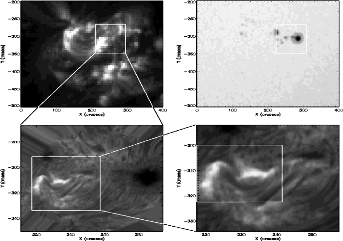 |
Figure 1:
Identification of analysed regions in NOAA8218.
Upper left panel: EIT 195 Å image taken at 14:51 UT. The SVST
field of view is overlaid
Upper right panel: MDI continuum image taken at 14:50:34 UT. The SVST
field of view is overlaid.
Lower left panel: SVST H |
| Open with DEXTER | |
| |
Figure 2:
Figure showing the locations of the main features discussed in the text. The flaring region A, and non-flaring region B, are marked on both images. Left panel: G band image at 14:32:30 UT. The two sunspots are denoted X and Y. Thread-like structures between them and close to X are marked. Right panel: H |
| Open with DEXTER | |
Figure 2 shows a G-band and H![]() line centre image taken at 14:32:30 UT and 14:34:00 UT, respectively.
This figure has been prepared in order to aid identification of the features that are discussed throughout this
paper. In the subsequent text, when we refer to, e.g., thread-like structures, we are referring to those
identified in this figure. The area shown is a 40.5 by 42.2 arcsec subregion cut out from the full field
of view as shown in Fig. 1. Solar North is up and East is to the left.
In both images two emerging flux regions (marked A and B) have been outlined. The flare studied in this
paper occurred in region A. In the G-band image, two sunspots (marked X and Y) are arrowed and in the H
line centre image taken at 14:32:30 UT and 14:34:00 UT, respectively.
This figure has been prepared in order to aid identification of the features that are discussed throughout this
paper. In the subsequent text, when we refer to, e.g., thread-like structures, we are referring to those
identified in this figure. The area shown is a 40.5 by 42.2 arcsec subregion cut out from the full field
of view as shown in Fig. 1. Solar North is up and East is to the left.
In both images two emerging flux regions (marked A and B) have been outlined. The flare studied in this
paper occurred in region A. In the G-band image, two sunspots (marked X and Y) are arrowed and in the H![]() image the approximate locations of the flare ribbons are arrowed (LR and RR). Below we discuss the relationship
between these features and the magnetic field. We also discuss the relationship between the dark thread-like
structures (arrowed in the G-band image) and the overlying H
image the approximate locations of the flare ribbons are arrowed (LR and RR). Below we discuss the relationship
between these features and the magnetic field. We also discuss the relationship between the dark thread-like
structures (arrowed in the G-band image) and the overlying H![]() inverted S-shaped structure (arrowed in
the H
inverted S-shaped structure (arrowed in
the H![]() image). Some arch filaments in region B have also been marked connecting the sunspot P and the
elongated dark sunspot O.
image). Some arch filaments in region B have also been marked connecting the sunspot P and the
elongated dark sunspot O.
Figure 3 shows the flare development in the H![]() line center and -700 mÅ blue wing.
The area shown is the same as in Fig. 2.
The Figs. show the
morphology of the dark filaments as they develop through the sequence.
At 13:38:04 UT there appear to be two or three arched structures interacting in
the image. Two curved structures (labelled numbers 1 and 2 in the image)
extend from the North-East towards
the image center and a further structure (number 3) curves from the center towards the West of
the image. It is not immediately clear whether this last structure is separate or
whether it is connected to number 1 in a twisted inverted S-shape underneath structure 2. As the
sequence progresses this inverted S-shape becomes more pronounced and structure 2 appears to merge with structure
3 or disappear.
By 14:48:12 UT only a single inverted S-shape remains clearly visible. As the flare occurs (see the image
at 14:52:55 UT) this inverted S-shape seems to separate such that two dark structures appear clearly
in the rest of the observations (e.g. labels 1 and 2 in the 14:57:34 UT image).
Such a scenario may be evidence for the stressing and shearing of twisted magnetic flux and subsequent separation after
magnetic reconnection disrupts the magnetic field in the corona. This is discussed further in Sect. 4.
The flare itself is of short
duration. Brightenings start to appear around the H
line center and -700 mÅ blue wing.
The area shown is the same as in Fig. 2.
The Figs. show the
morphology of the dark filaments as they develop through the sequence.
At 13:38:04 UT there appear to be two or three arched structures interacting in
the image. Two curved structures (labelled numbers 1 and 2 in the image)
extend from the North-East towards
the image center and a further structure (number 3) curves from the center towards the West of
the image. It is not immediately clear whether this last structure is separate or
whether it is connected to number 1 in a twisted inverted S-shape underneath structure 2. As the
sequence progresses this inverted S-shape becomes more pronounced and structure 2 appears to merge with structure
3 or disappear.
By 14:48:12 UT only a single inverted S-shape remains clearly visible. As the flare occurs (see the image
at 14:52:55 UT) this inverted S-shape seems to separate such that two dark structures appear clearly
in the rest of the observations (e.g. labels 1 and 2 in the 14:57:34 UT image).
Such a scenario may be evidence for the stressing and shearing of twisted magnetic flux and subsequent separation after
magnetic reconnection disrupts the magnetic field in the corona. This is discussed further in Sect. 4.
The flare itself is of short
duration. Brightenings start to appear around the H![]() ribbon locations
around 14:43 and are visible in the 14:48:12 UT image.
The flare ribbons reach maximum intensity simultaneously at 14:52:55 UT and
the main phase is already over by 14:57:34 UT although low level
brightenings continue to occur throughout the rest of the observing sequence.
In the notation introduced above, LR refers to the location of the left (Eastern) ribbon and RR to the location of the right (Western) ribbon.
North West of RR there is an elongated structure (O) which appears connected by
H
ribbon locations
around 14:43 and are visible in the 14:48:12 UT image.
The flare ribbons reach maximum intensity simultaneously at 14:52:55 UT and
the main phase is already over by 14:57:34 UT although low level
brightenings continue to occur throughout the rest of the observing sequence.
In the notation introduced above, LR refers to the location of the left (Eastern) ribbon and RR to the location of the right (Western) ribbon.
North West of RR there is an elongated structure (O) which appears connected by
H![]() filaments to a spot (P) just to the South West of RR. In Sects. 3.1 and 3.2 we discuss the temporal development and interactions of these regions which may provide the key to the
production of the flare. The areas of the regions are those marked A and B in Fig. 2 and contours have also
been overlaid on the 14:38:53 UT H
filaments to a spot (P) just to the South West of RR. In Sects. 3.1 and 3.2 we discuss the temporal development and interactions of these regions which may provide the key to the
production of the flare. The areas of the regions are those marked A and B in Fig. 2 and contours have also
been overlaid on the 14:38:53 UT H![]() image in Fig. 4.
image in Fig. 4.
Figure 4 shows the development of the emerging flux region in the G-band, magnetogram and
H![]() line center images before and after the flare. The area shown is the same as Fig. 3.
The example images shown cover the period 12:48:26 UT to 16:22:13 UT and were selected for their quality. The images are interspersed with examples of magnetogram contours overlaid on nearly time-coincident G-band and H
line center images before and after the flare. The area shown is the same as Fig. 3.
The example images shown cover the period 12:48:26 UT to 16:22:13 UT and were selected for their quality. The images are interspersed with examples of magnetogram contours overlaid on nearly time-coincident G-band and H![]() images (see the images labelled with B/H
images (see the images labelled with B/H![]() and B/G).
In these images white indicates positive polarity and black indicates negative
polarity. The main contour level is 400 G. However, in the flaring region, an additional contour at 220 G
has also been plotted to better reveal the lower magnetic flux structures
discussed below.
and B/G).
In these images white indicates positive polarity and black indicates negative
polarity. The main contour level is 400 G. However, in the flaring region, an additional contour at 220 G
has also been plotted to better reveal the lower magnetic flux structures
discussed below.
Comparison of the initial and final G-band images
at 12:49:33 UT and 16:20:13 UT indicates that the region is one of emerging flux.
Clearly there is a growth in the
number of dark regions confirmed also by an increase in the number of areas of concentrated
magnetic flux in the magnetograms at 13:08:16 UT and 16:22:13 UT.
From the 14:55:53 UT G-band image with overlaid magnetic flux contours it is clear that
the two sunspots (noted as X and Y in Fig. 2) are associated with magnetic flux of opposite
polarities. Note the white positive magnetic flux contours encircling X and the black
negative polarity contours encircling Y. From the 14:55:53 UT H![]() image with
overlaid magnetic flux contours it is also clear that the H
image with
overlaid magnetic flux contours it is also clear that the H![]() flare ribbons
are located on top of and around these opposite polarity sunspots. Note how the flare ribbon
(denoted LR above) occurs over and to the South of the white positive polarity contours associated
with sunspot X, and the flare ribbon (denoted RR above) occurs over the black negative
polarity contours associated with sunspot Y.
The same features are visible in the Ca II K-line data (not shown here)
prior to the flare but are masked by the
brightenings seen at the flare peak time. We examined the spatial locations of the H
flare ribbons
are located on top of and around these opposite polarity sunspots. Note how the flare ribbon
(denoted LR above) occurs over and to the South of the white positive polarity contours associated
with sunspot X, and the flare ribbon (denoted RR above) occurs over the black negative
polarity contours associated with sunspot Y.
The same features are visible in the Ca II K-line data (not shown here)
prior to the flare but are masked by the
brightenings seen at the flare peak time. We examined the spatial locations of the H![]() flare
ribbons using contour overlays and found that although the flare is more intense in the H
flare
ribbons using contour overlays and found that although the flare is more intense in the H![]() image than in the K-line
image, the K-line brightenings appear well correlated with the H
image than in the K-line
image, the K-line brightenings appear well correlated with the H![]() ribbons.
These findings are consistent with the footpoints being
heated by the bombardment of high energy
electrons and/or thermal conduction. The structure connecting the footpoints could have pre-existed or been formed
during magnetic reconnection.
ribbons.
These findings are consistent with the footpoints being
heated by the bombardment of high energy
electrons and/or thermal conduction. The structure connecting the footpoints could have pre-existed or been formed
during magnetic reconnection.
The 14:55:53 UT G-band image with magnetic flux contour overlays also shows that the H![]() arch filaments
in region B
connecting the elongated dark region, O, and the sunspot, P, are rooted in opposite polarities. Black negative
polarity contours encircle O and white positive polarity contours encircle P.
arch filaments
in region B
connecting the elongated dark region, O, and the sunspot, P, are rooted in opposite polarities. Black negative
polarity contours encircle O and white positive polarity contours encircle P.
Note the dark thread-like regions between the two spots and to the right of the spot denoted X
(circled in the 12:49:33 UT G-band image).
These thread-like structures grow, develop
and darken
throughout the G-band sequence of images and do not appear to be related
to the brightenings in H![]() .
The thread-like structures appear nearly perpendicular to
the centre-to-centre line connecting the two opposite polarity sunspots.
However, by comparing the 13:21 and 14:32 UT G-band images, it is possible to see that the
orientation of these features changes so that they are pointed further towards the South East i.e.
the angle with the centre-to-centre line even increases before the flare.
In Sect. 3.2 we demonstrate that these dark structures relate to magnetic
flux which is emerging between the two main spots. These structures are of a comparatively
lower magnetic flux which can only be seen through reducing the dynamic range
of the magnetograms (as discussed
above). This may also imply that they are mainly horizontal structures with a lower
longitudinal magnetic field.
These findings indicate that the emergence of new magnetic flux almost perpendicular
to the overlying magnetic field developed a strongly sheared magnetic field configuration,
as evidenced by the inverted S-shaped filament, and caused the flare.
.
The thread-like structures appear nearly perpendicular to
the centre-to-centre line connecting the two opposite polarity sunspots.
However, by comparing the 13:21 and 14:32 UT G-band images, it is possible to see that the
orientation of these features changes so that they are pointed further towards the South East i.e.
the angle with the centre-to-centre line even increases before the flare.
In Sect. 3.2 we demonstrate that these dark structures relate to magnetic
flux which is emerging between the two main spots. These structures are of a comparatively
lower magnetic flux which can only be seen through reducing the dynamic range
of the magnetograms (as discussed
above). This may also imply that they are mainly horizontal structures with a lower
longitudinal magnetic field.
These findings indicate that the emergence of new magnetic flux almost perpendicular
to the overlying magnetic field developed a strongly sheared magnetic field configuration,
as evidenced by the inverted S-shaped filament, and caused the flare.
Having established that the flare ribbons LR and RR occur on top of and around the sunspots X and Y, we use the labels LR and RR throughout the rest of the paper. From Fig. 4 and from the movies we generated we noted an interesting movement of RR towards LR. This is an unusual motion for an emerging flux region and may be evidence of twisting of the magnetic field. We return to this point in Sect. 3.2.
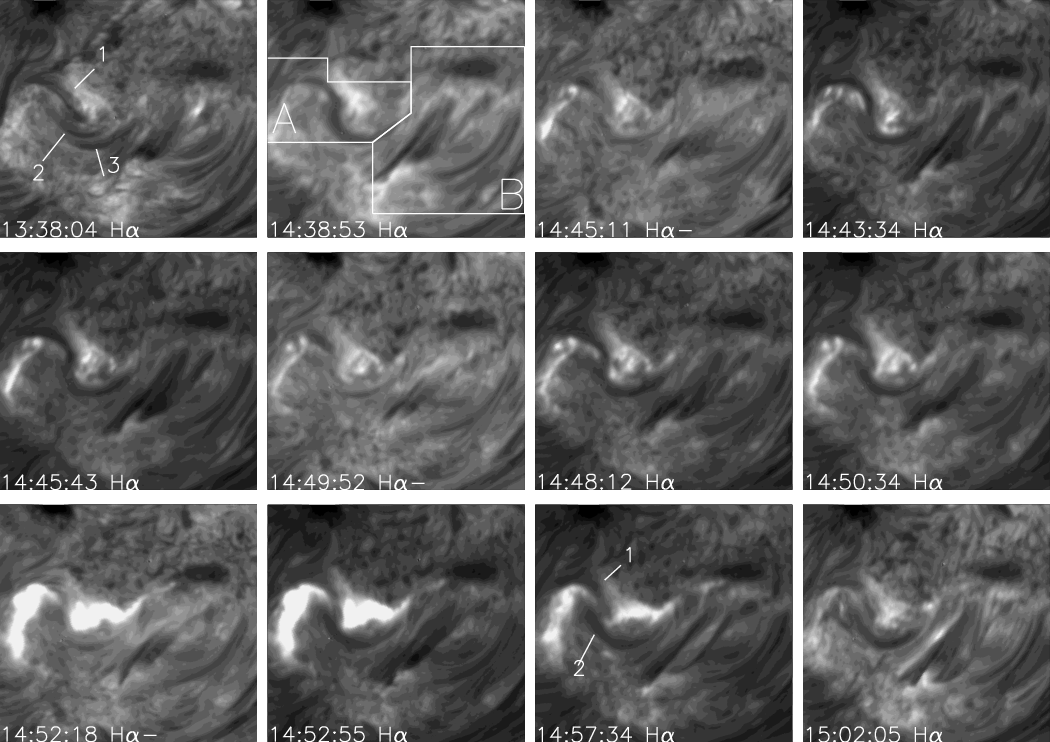 |
Figure 3:
40.5
|
| Open with DEXTER | |
 |
Figure 4:
40.5
|
| Open with DEXTER | |
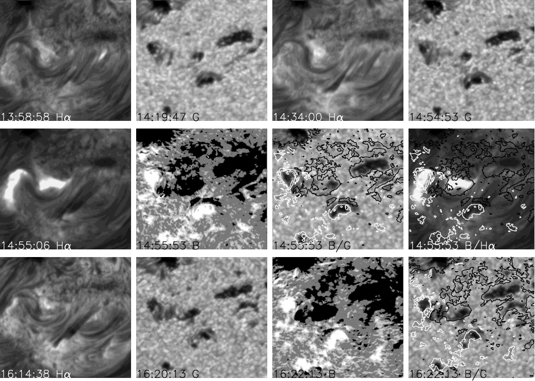 |
Figure 4: continued. |
| Open with DEXTER | |
Figure 5 shows light curves for the H![]() line center and -700 mÅ blue wing. The cutout region is a
line center and -700 mÅ blue wing. The cutout region is a ![]() 23.7 by 22.0 arcsec subregion shown as a box on the 14:52:55 UT image of Fig. 1 (lower right hand panel). The area was chosen
to include the full extent of the H
23.7 by 22.0 arcsec subregion shown as a box on the 14:52:55 UT image of Fig. 1 (lower right hand panel). The area was chosen
to include the full extent of the H![]() flare ribbons.
The flux is the total flux within
the region, in arbitrary units (right hand y-axis).
Universal time is given in 10 minute intervals along the x-axis
from 14:10 UT until 15:50 UT. The curves are labelled as H
flare ribbons.
The flux is the total flux within
the region, in arbitrary units (right hand y-axis).
Universal time is given in 10 minute intervals along the x-axis
from 14:10 UT until 15:50 UT. The curves are labelled as H![]() and H
and H![]() -.
-.
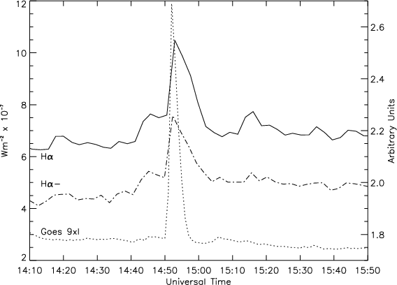 |
Figure 5:
GOES-9 1 min X-ray flux light curves. The left y-axis is in flux units of Wm
|
| Open with DEXTER | |
The GOES-9 (Geosynchronous Operational Environmental Satellites)
1 min X-ray flux light curve in the XL band (1-8 Å) has been overplotted.
The flux units are Wm
![]() (left y-axis).
The flare is clearly visible in each curve and as with H
(left y-axis).
The flare is clearly visible in each curve and as with H![]() the GOES X-ray flux peaks at 14:52 UT. The GOES classification for the X-ray flux peak is C1.1.
The X-ray flare duration is approximately 8 min which is slightly shorter
than in H
the GOES X-ray flux peaks at 14:52 UT. The GOES classification for the X-ray flux peak is C1.1.
The X-ray flare duration is approximately 8 min which is slightly shorter
than in H![]() (
(![]() 20 min).
20 min).
The main phase of the flare shows a typical impulsive nature in both wavelengths.
A precursor brightening can be seen in H![]() ;
it starts around 14:42 UT and attains a small
peak around 14:46 UT. The GOES flux shows no obvious brightening at this time, but shows fluctuations consistent
with the fluctuations in the H
;
it starts around 14:42 UT and attains a small
peak around 14:46 UT. The GOES flux shows no obvious brightening at this time, but shows fluctuations consistent
with the fluctuations in the H![]() curve. These precursor brightenings in H
curve. These precursor brightenings in H![]() are identified as small bright points located close to the sheared filament in both the opposite polarity regions.
The first brightening occurred at 13:21 UT and many other points successively brightened until 14:50:34 UT and then
explosively flashed at the 14:52 UT main peak. Note that we find neither filament motion
nor separating motion of the two flare ribbons in this flare, unlike the typical dynamical flare
(Kurokawa 1987).
are identified as small bright points located close to the sheared filament in both the opposite polarity regions.
The first brightening occurred at 13:21 UT and many other points successively brightened until 14:50:34 UT and then
explosively flashed at the 14:52 UT main peak. Note that we find neither filament motion
nor separating motion of the two flare ribbons in this flare, unlike the typical dynamical flare
(Kurokawa 1987).
Figures 6 and 7 show the development of the magnetic field in regions A and B.
The average magnetic flux is calculated for each time in the sequence and the results are displayed as the
upper left (positive) and lower left (negative) plots in Fig. 6 for the flaring region (A) and Fig. 7 for the
non-flaring region (B). The aproximate duration of the
H![]() flare
together with the time of peak emission are also shown.
Since the magnetograms do not give us any information on the magnetic field
strength above 1800 G this average is a lower limit to the real average. However, we can make an estimate
of the accuracy of the average by recording those pixels with values of greater than or equal to 1800 G.
We call these "saturated pixels'' and the % of the total number of pixels within the area which are saturated is
shown for each time in the upper right (positive) and lower right (negative) plots associated with the respective figures.
flare
together with the time of peak emission are also shown.
Since the magnetograms do not give us any information on the magnetic field
strength above 1800 G this average is a lower limit to the real average. However, we can make an estimate
of the accuracy of the average by recording those pixels with values of greater than or equal to 1800 G.
We call these "saturated pixels'' and the % of the total number of pixels within the area which are saturated is
shown for each time in the upper right (positive) and lower right (negative) plots associated with the respective figures.
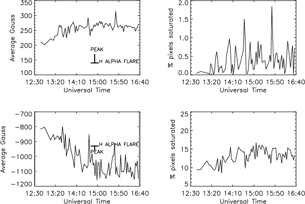 |
Figure 6: Time development of average magnetic flux and the percentage of saturated pixels for the flaring region (A in Fig. 4). Upper left - average Gauss (+ve). Lower left - average Gauss (-ve). Upper right - % of pixels saturated (+ve). Lower right - % of pixels saturated (-ve). |
| Open with DEXTER | |
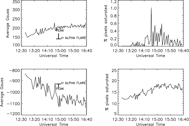 |
Figure 7: Time development of average magnetic flux and the percentage of saturated pixels for the non-flaring region (B in Fig. 4). Upper left - average Gauss (+ve). Lower left - average Gauss (-ve). Upper right - % of pixels saturated (+ve). Lower right - % of pixels saturated (-ve). |
| Open with DEXTER | |
In the case of the positive polarity flaring region the total % of pixels which are saturated does not exceed 2.0%. In the case of the negative polarity flaring region the total is substantially larger but does not exceed 17%. In the emerging region to the West the total % of pixels which are saturated is less than 1.2% for the positive polarity region and less than 20% for the negative polarity region.
Figure 4 also clearly shows that the positive and negative flux within regions A and B are clearer and more intense in the last magnetogram than in the first. Figures 6 and 7 show that the positive polarity region is slightly stronger in the flaring region, A, than in the non-flaring region, B, but that the negative polarity region in the non-flaring region is similar in strength to that in the flaring region. In both A and B the negative polarity region is stronger than the positive polarity region. In addition, the average Gauss of both polarities in both regions increases prior to the flare before apparently levelling off. The positive values increase by a factor of around 1.3 and 1.2 by the time of the flare for the flaring and non-flaring region, respectively. The negative values also increase by a factor of about 1.3 and 1.2 for the two regions by the same time. Also, the percentage of the total number of positive polarity points which saturate increases during this period from 0 to about 1.5% for region A and from 0 to about 1.0% for region B, while the total number of negative polarity points which saturate increases from about 10 to 15% for the flaring region and from 12 to 17% for the non-flaring region. Note also that a secondary effect of the increase in pixel saturation is that the factor increases quoted for the average Gauss will be lower limits.
Even though there is some difference in the strength of the positive and negative magnetic flux in the two regions and the rate of increase may be slightly faster in the flaring region, the time development is qualitatively similar. The important point to note is that all three pieces of evidence indicate that both the positive and negative flux is increasing (i.e. magnetic flux is emerging) in both the flaring and non-flaring regions, at least until the flare onset time. This suggests that we must consider other possibilities as to why only one of the regions should produce a flare.
In order to track the movement of the various features in the flare region we used three separate techniques; timeslices, small feature tracking and a local correlation tracking method (LCTM).
Figure 8 shows timeslice images, in region A, which demonstrate the movement of
the negative polarity spot RR towards the positive polarity spot LR.
The lower left image of the figure is taken from
the G band data at 12:49:33 UT and the upper left magnetogram was taken at 12:44:28 UT. Both images are 40.5 by 42.2 arcsec cutout areas covering the region shown in Fig. 4. A number of "slice-lines'' of varying directions were tested to accurately assess the movement of the spot. The absicca of the coordinate frame of the right hand image shows the pixel position along the slice-line and the ordinate shows the time. The chosen slice-line is overplotted on the two left hand images and is the same for both the G band data
and the magnetograms.
The positive polarity spot therefore sits towards the left hand end of the slice-line near
pixel 0 in the slice-image. The negative polarity spot is located
close to the right hand side of the slice-line which corresponds to pixel 148 in the slice-image.
The slice-image clearly shows that the negative polarity
region moves along the line so that the leading edge has moved from around pixel 107 to around pixel 93.
The trailing edge of the positive polarity spot also moves a little along the slice-line from around pixel 32.5 to around pixel 29.5.
Assuming that 1 arcsec represents approx. 725 km
on the Sun's surface this relative
distance of 11 pixels corresponds to ![]() 794 km and hence a relative velocity of
794 km and hence a relative velocity of ![]() 59 m s-1.
This result indicates that if the two spots are magnetically connected, then some shearing of the
magnetic neutral line must occur. Note also the stability of the positive polarity spot (the darkest line to the left of the
slice image).
59 m s-1.
This result indicates that if the two spots are magnetically connected, then some shearing of the
magnetic neutral line must occur. Note also the stability of the positive polarity spot (the darkest line to the left of the
slice image).
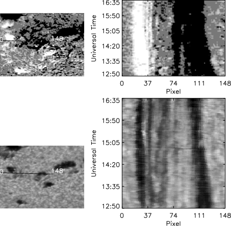 |
Figure 8: Timeslice image showing the movement of RR towards LR (see text). The image on the lower left of the figure is taken from the G-band data at 12:49:33 UT and the magnetogram in the upper left was taken at 12:44:28 UT. Both are 42.2 by 42.2 arcsec in size. The slice-line is overlaid and the starting pixel (0) and ending pixel (148) are also shown. The absicca of the coordinate frame of the right hand plot shows the same pixel position along the slice-line. The ordinate shows the time. |
| Open with DEXTER | |
Figure 9 contrasts the development of the non-flaring region, B, with that of the flare region A. The G-band image and magnetogram are the same as before. Again a number of slice-lines were used to accurately assess the direction of movement. Pixel 0 on the slice-line is positioned just ahead of the direction of motion of the positive polarity region, P, and pixel 179 is ahead of the direction of movement of the negative polarity region, O. The dark regions in the G band image show indications of a separating motion which appears more obvious in the timeslice of the magnetogram. The negative polarity feature associated with the upper spot (around pixel 134) clearly moves while the movement of the positive polarity region (around pixel 44) is less obvious. However, even a slightly curved separating path, similar to the shape of the path in the G band timeslice, can be discerned. A bipolar sunspot is also seen moving between the two main spots.
Consider now the darkening of the area between the spots in Fig. 8 (around pixels 37 to 56). We investigated this region in further detail and two further timeslices are shown in Figs. 10 and 11. This time the G band image was taken at 13:35:52 UT and the magnetogram at 13:36:20 UT. These times were chosen in order to examine the relationship between the magnetic field and the dark regions. These regions correspond to the thread-like structures discussed earlier which are visible between the two spots and are emerging almost perpendicular to the line connecting the opposite polarity sunspots. By 13:30 considerable darkening between the spots had already occurred and the thread-like structures are quite well defined (compare this image with the one in Fig. 8, for example). Of course, this darkening is itself clear evidence of emerging flux.
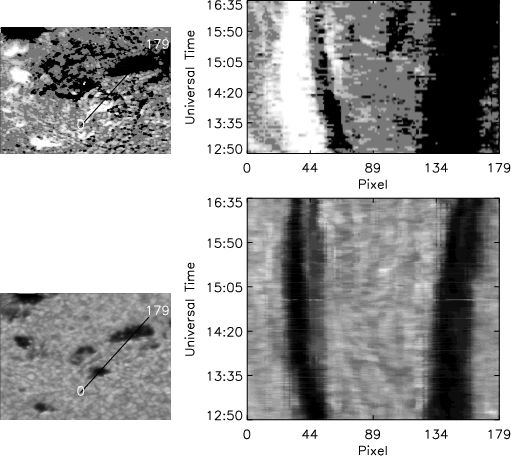 |
Figure 9: Timeslice image showing the separation of the structures in the non-flaring region, B. The G-band image and magnetogram are the same as before. The slice-line is overlaid and the starting pixel (0) and ending pixel (179) are also shown. The absicca of the coordinate frame of the right hand plot shows the same pixel position along the slice-line. The ordinate shows the time. |
| Open with DEXTER | |
In Fig. 10, we examined the right hand thread. The upper end of the slice-line in this figure corresponds to pixel 0 and the lower end corresponds to pixel 112. By comparison of these timeslice images and the contour overlays in Fig. 4 we determined that this thread is associated with predominantly positive magnetic flux but with a negative polarity region at its lower end. These positive polarity regions appear to separate when observed in the movies and this is reflected in the magnetic field time slice. These observations are consistent with the general picture of emerging flux: when a magnetic flux rope has emerged above the photosphere, the expansion of the structure naturally causes the magnetic footpoints to separate. However, while the right hand dark structure (around pixel 70) appears to be associated directly with negative magnetic flux the positive flux appears to be at the boundary of the thread and the surrounding region (compare the position of the left edge of the dark region in the G band timeslice with the positive separating flux in the magnetic field time slice).
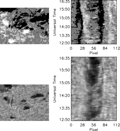 |
Figure 10: Timeslice image showing emerging flux between LR and RR. The G-band image in this figure was taken at 13:35:52 UT and the magnetogram was taken at 13:36:20 UT. The slice-line is overlaid and the starting pixel (0) and ending pixel (112) are also shown. The absicca of the coordinate frame of the right hand plot shows the same pixel position along the slice-line. The ordinate shows the time. |
| Open with DEXTER | |
In Fig. 11, we examined the left hand thread. The upper end of the slice-line in this figure corresponds to
pixel 0 and the lower end corresponds to pixel 84.
Again by comparison of these timeslices and the contour overlays of Fig. 4 we determined that this thread is associated
almost exclusively with positive magnetic flux. The dark negative flux that appears in the timeslice around pixel 63 at around
14:10 UT seems to correspond to separate flux moving onto the slice-line from the West.
This feature also appears to be curving around the main positive spot. In fact although both thread structures appear to initially
emerge almost perpendicular to the line connecting the main spots, the angle between the threads and this line appears to increase
before the flare as discussed in Sect. 3. The difficulty in relating the G band and magnetic features is mainly due to the
variability in seeing conditions and low field strength in this region. However, these results
suggest that this emerging flux developed a sheared magnetic field configuration with the overlying field,
as indicated by the inverted S-shaped H![]() filament, and caused the flare.
filament, and caused the flare.
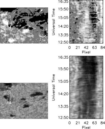 |
Figure 11: Timeslice image showing emerging flux between LR and RR. The G-band image in this figure was taken at 13:35:52 UT and the magnetogram was taken at 13:36:20 UT. The slice-line is overlaid and the starting pixel (0) and ending pixel (84) are also shown. The absicca of the coordinate frame of the right hand plot shows the same pixel position along the slice-line. The ordinate shows the time. |
| Open with DEXTER | |
Figure 12 shows a time-slice with a similar orientation to Fig. 8 but using SOHO/MDI full disk data. Although the data is of lower resolution it enables us to both cover the SVST observations period and investigate the development of the region after 17 UT. In this figure the time-slice is extended to 05 UT on May 14. It clearly shows the approach of the negative polarity region to the positive polarity region. Note also that it continues to approach even after the flare has occurred. Later the two spots appear to maintain their separation and analysis of further data up to 17 UT shows that the negative polarity spot also seems to change direction around 5 or 6 UT and eventually positioned itself to the South of the positive polarity spot. Finally the two spots disappear from MDI white light images around 06 UT on the 15th. This information is important when considering the discussion of Sect. 4.
| |
Figure 12: Timeslice image showing the movement of the positive and negative polarity spots from SOHO/MDI data. The timeslice covers the SVST observations period and extends much later until around 05:00 UT on May 14th. |
| Open with DEXTER | |
Having established the general motion of the large regions we applied feature tracking and correlation analysis to the dataset.
The LCTM was applied to an area of 81
![]() by 84.6
by 84.6
![]() around the region of interest.
The method adopted derives the velocity structure
from the dataset by tracking correlations between image sub-areas within a pre-defined box
size, search area and temporal distance. These parameters are determined by reducing the difference
between results obtained from an even-odd test. That is, results are obtained for a dataset of odd numbered images
and also for a dataset of even numbered images. The differences between the results are compared
and the parameters which best reduce this difference are selected. For our dataset this procedure
produced a box size of 10 by 10 pixels (3.38
around the region of interest.
The method adopted derives the velocity structure
from the dataset by tracking correlations between image sub-areas within a pre-defined box
size, search area and temporal distance. These parameters are determined by reducing the difference
between results obtained from an even-odd test. That is, results are obtained for a dataset of odd numbered images
and also for a dataset of even numbered images. The differences between the results are compared
and the parameters which best reduce this difference are selected. For our dataset this procedure
produced a box size of 10 by 10 pixels (3.38
![]() by 3.38
by 3.38
![]() ), a temporal distance of 120 s on average and
a search area of 5 pixels. This last parameter is large enough to trace features with velocities of 9.8 km s-1 and
is also enough to track motions due to seeing. It is also sufficiently small to exclude correlations with
distant boxes.
), a temporal distance of 120 s on average and
a search area of 5 pixels. This last parameter is large enough to trace features with velocities of 9.8 km s-1 and
is also enough to track motions due to seeing. It is also sufficiently small to exclude correlations with
distant boxes.
The results are combined in Fig. 13 which is a composite of several images. The main plot and scale is the velocity map. The numbers on the x/y-axes are simply labels separated by the box width/height to give a reference position when referring to the various features. Since the box width is 10 pixels the 240 by 250 pixel image is divided into 24 by 25 boxes. The arrows shows the direction of motion of each box and their magnitudes are proportional to the distance travelled by the box although the absolute value is arbitrary. The underlying image is the divergence image. White areas are regions of positive divergence and dark areas are regions of negative divergence i.e. convergence. The brighter/darker the region the greater the divergence/convergence. For example, the maximum divergence is found around position (4, 3). Contours of the G band dark spots are overplotted with levels of 0.195% and 0.390%.
![\begin{figure}
\par\includegraphics[width=8.8cm,clip]{3354f13.eps}
\end{figure}](/articles/aa/full/2003/45/aa3354/img20.gif) |
Figure 13: Results from the local correlation tracking method. The size of the area is the same as Figs. 3 and 4. The velocity map is plotted and the magnitude of the arrows are proportional to the distance travelled by the corresponding box although the absolute value is arbitrary (see text). The arrowhead gives the direction of motion. The underlying image image is the divergence map. White areas are regions of positive divergence and dark areas are regions of convergence. Contours of the G band dark spots are also overplotted with levels of 0.195% and 0.390%. |
| Open with DEXTER | |
The results confirm and extend the findings from the timeslice method. The maximum, average and minimum velocities
over the whole observing period (3h46m57s) are 1.679, 0.4729 and 0.02884 km s-1, respectively.
There is a clear divergence in the
region where flux is emerging between LR and RR supported also by strong velocity flows.
Since the box size is small it is effective at
tracking this motion. RR also shows large velocity arrows at its trailing
edge and dark convergence regions between it and LR. Along the line chosen for the time slice
analysis of Fig. 7 their is initial convergence before it is overwhelmed by divergence from the region
emerging parallel to the neutral line. This is consistent with the timeslice results as RR does
not approach this close to LR throughout the sequence. The LCTM method also reveals
the separating motion of the two G band dark spots O and P in the non-flaring region. As mentioned
these regions are
connected by dark loop structures in the H![]() data.
There is
also a constant stream of short-lived bright points in both the G band and K-line datasets
(not presented here)
in this area which seem to move between RR and spot P and also around
the latter spot and almost parallel to the lower edge of the elongated dark structure, O.
More precisely, the flows are not obviously perpendicular to the neutral line between these features
as one might expect from an emerging structure. The flows may also have some influence on the movement
of RR towards LR.
data.
There is
also a constant stream of short-lived bright points in both the G band and K-line datasets
(not presented here)
in this area which seem to move between RR and spot P and also around
the latter spot and almost parallel to the lower edge of the elongated dark structure, O.
More precisely, the flows are not obviously perpendicular to the neutral line between these features
as one might expect from an emerging structure. The flows may also have some influence on the movement
of RR towards LR.
Note that Fig. 13 shows almost no velocity motion at the flare site between the positions of the
H![]() flare ribbons and that the divergence image shows no strong convergent or divergent flows.
flare ribbons and that the divergence image shows no strong convergent or divergent flows.
Feature tracking was also applied interactively selecting regions in the images and visually following their motion through the dataset. This was found to be very effective for following the motion of the larger spots. In the case of smaller features, such as G-band bright points, the technique was of limited effectiveness in the area of interest around the flare site due to the lack of motion in this region and the short duration of the brightenings. However, it was possible to identify and track longer duration brightenings and movements such as the flow pattern between RR and the spot P evident in the LCTM results discussed above. The feature tracking results were substantially the same as the those of the timeslice and LCTM procedures and so have been omitted for brevity.
Figure 14 shows a close-up image of the flare region at the time of peak intensity
(14:50:57 UT) obtained by EIT (Fe XII ![]() 195 Å). The image corresponds to the SVST FOV as shown in Fig. 1 and is 84 by 84 arcsec.
An MDI magnetogram has been overlaid on the close-up to aid in cross-identification of features with the SVST dataset.
The magnetogram was taken at 14:58:05 UT. Positive polarity regions are denoted by dashed contours and negative polarity regions are denoted by solid contours. Figure 15 shows an SVST H
195 Å). The image corresponds to the SVST FOV as shown in Fig. 1 and is 84 by 84 arcsec.
An MDI magnetogram has been overlaid on the close-up to aid in cross-identification of features with the SVST dataset.
The magnetogram was taken at 14:58:05 UT. Positive polarity regions are denoted by dashed contours and negative polarity regions are denoted by solid contours. Figure 15 shows an SVST H![]() line center image taken just after the
flare peak at 14:57:34 UT (closest in time to the EIT and MDI images). The EIT
image has been overlaid as solid contours to show the locations of the brightenings. The contour surrounding LR is about 50% of the peak intensity of RR. A Yohkoh-SXT image taken at 14:56:06 UT is also overlaid as dashed contours.
The percentages for the contour levels are the same in both overlays i.e.
20%, 50%, 80% and 100% of the peak intensity of the image.
The images have been processed using EIT and MDI procedures
together with D. Zarro's IDL mapping software, both available in SolarSoft.
line center image taken just after the
flare peak at 14:57:34 UT (closest in time to the EIT and MDI images). The EIT
image has been overlaid as solid contours to show the locations of the brightenings. The contour surrounding LR is about 50% of the peak intensity of RR. A Yohkoh-SXT image taken at 14:56:06 UT is also overlaid as dashed contours.
The percentages for the contour levels are the same in both overlays i.e.
20%, 50%, 80% and 100% of the peak intensity of the image.
The images have been processed using EIT and MDI procedures
together with D. Zarro's IDL mapping software, both available in SolarSoft.
![\begin{figure}
\par\includegraphics[width=7cm,clip]{3354f14.eps}
\end{figure}](/articles/aa/full/2003/45/aa3354/img21.gif) |
Figure 14: EIT 195 Å image of NOAA 8218 at the time of flare peak intensity (14:50:57 UT). corresponding to the SVST field of view as shown by the box on the EIT image in the upper left hand panel of Fig. 1. An MDI magnetogram has been overlaid to aid in cross identification of features with the SVST dataset. The magnetogram was taken at 14:58:05 UT. Positive polarity regions are denoted by dashed contours and negative polarity regions are denoted by solid contours. |
| Open with DEXTER | |
![\begin{figure}
\par\includegraphics[width=6cm,clip]{3354f15.eps}
\end{figure}](/articles/aa/full/2003/45/aa3354/img22.gif) |
Figure 15:
SVST H |
| Open with DEXTER | |
The MDI contours are in arbitrary units at intervals of 100 between 100 and 1100. Positive polarity regions are denoted by dashed contours and negative polarity regions are denoted by solid contours.
The EIT image shows the flare site in the ultraviolet wavelength range at plasma temperatures of around 1.4 MK. Interestingly the peak intensity appears to lie close to the negative polarity (RR) spot in the MDI images and this is not an effect of the time difference between images as it retains the same location in later MDI magnetograms. Recall that Fig. 1 image also shows extensive larger bright features which can be identified as portions of coronal loops connecting from the predominantly negative region to a largely positive region outside the SVST field of view but visible with EIT/MDI. For example, consider the low level contour below the flare site in Fig. 15. Figure 1 shows that it is clearly identified as the lower part of a larger loop structure(s).
The precise locations of the foot points of these larger loops are not easily established as the EIT spatial resolution is not high enough for a detailed comparison with the SVST data. However, the coronal loop seems to cross above the emerging flux region at an angle perpendicular to the neutral line. Recall that magnetic flux is also emerging in this direction between the flare ribbons. This then might suggest that the flare is a product of interacting loops in a magnetic quadrupole configuration (see e.g. Aschwanden et al. 1999 and references therein) or, alternatively, in a similar scenario to that proposed for homologous flares by Ranns et al. (2000) i.e. an emerging loop/overlying loop interaction.
We also derived the emission measure for the soft X-ray brightening using procedures developed for
Yohkoh and available in SolarSoft under the SXT branch.
The SXT image was taken with the AlMg filter.
However, unfortunately we could not use the filter ratio method of Hara et al. (1992) as the closest
image in time taken by a different filter was around 20 min before the flare onset.
Therefore we resorted to assuming an average temperature for the post flare X-ray loops of around 10MK. This
value is representative for post flare loops according to Kamio et al. (2003). The region of the flare was defined as the area where the intensity is greater than 10% of the peak intensity i.e. 1428 DN s-1 pixel-1. Under this criterion we find an area of ![]()
![]() cm2. From the total intensity of this region we derived a volume emission measure of
cm2. From the total intensity of this region we derived a volume emission measure of ![]()
![]() cm-3. If we assume that the flare brightening depth is proportional to the square root of the surface area then the volume is
cm-3. If we assume that the flare brightening depth is proportional to the square root of the surface area then the volume is
![]() cm3 and hence the density is
cm3 and hence the density is
![]() cm-3. Of course if the filling factor is less than unity then the density will be correspondingly higher.
cm-3. Of course if the filling factor is less than unity then the density will be correspondingly higher.
Assuming this density we can make a simple estimate of the
thermal energy content via
![]() ,
where
,
where ![]() is the electron density, EM is the volume emission measure,
is the electron density, EM is the volume emission measure, ![]() is the electron temperature and
is the electron temperature and ![]() is Boltzmann's constant. We derive a value of
is Boltzmann's constant. We derive a value of
![]() ergs. The magnetic energy can then be estimated as
ergs. The magnetic energy can then be estimated as
![]() ergs from the relation
ergs from the relation
![]() (see e.g. Shibata & Yokoyama 2002).
(see e.g. Shibata & Yokoyama 2002).
First let us summarise our observational findings.
Figure 16 shows a schematic model of the emergence of twisted magnetic flux which we propose to account for these
observations. The figure shows a twisted magnetic flux tube and connecting "branch" emerging above the photosphere.
The box cut through the structure indicates the position of the photosphere at two different times in the
observing sequence. As the flux tube emerges its footpoints will initially separate. However, the schematic
model is designed such that the tube above LR is vertical and the tube above RR
is twisted to an half ![]() shape. Hence, at a later time, LR is still
located at the same position but RR has an apparent motion towards LR.
Since the angle of approach is not quite center to center the structure must twist (at least initially)
to the south of LR. To establish the subsequent motion of RR we checked MDI full disk continuum and magnetogram data
(some of which is shown in Fig. 12) and
found that RR continued to approach LR several hours after the SVST observations were completed eventually
stabilising in position near LR before they both disappear. This is the
reason our main flux tube takes the shallower line and direction in the figure.
shape. Hence, at a later time, LR is still
located at the same position but RR has an apparent motion towards LR.
Since the angle of approach is not quite center to center the structure must twist (at least initially)
to the south of LR. To establish the subsequent motion of RR we checked MDI full disk continuum and magnetogram data
(some of which is shown in Fig. 12) and
found that RR continued to approach LR several hours after the SVST observations were completed eventually
stabilising in position near LR before they both disappear. This is the
reason our main flux tube takes the shallower line and direction in the figure.
![\begin{figure}
\par\includegraphics[width=8cm,clip]{3354f16.eps}
\end{figure}](/articles/aa/full/2003/45/aa3354/img36.gif) |
Figure 16: Schematic drawing of emerging twisted magnetic flux tube as discussed in the text. |
| Open with DEXTER | |
A connecting "branch" is also shown twisting in an inverted S-shape from one trunk of the flux tube in an upward
and then downward direction to attach to the other trunk.
Initially none of this "branch" is observed but at a later time
dark structures are seen emerging parallel to the neutral line and close to LR. As the structures emerge the footpoints separate (as observed in the time slice Fig. 10). The magnetic field strength
is lower in this region so the field lines close to the strong positive polarity branch may obscure any weak
magnetic flux associated with the emerging branch which does not show any separating motion (Fig. 11). Alternatively,
the weak longitudinal field may suggest that the branch mainly has a horizontal magnetic component.
At greater heights in the atmosphere
H![]() dark filaments are located along the neutral line close to the field lines of the main twisted structure. The
emergence of this branch almost perpendicular to the overlying bipolar field along the main flux rope, causes a quick
development of a sheared magnetic field configuration which is observed as the inverted S-shaped structure in H
dark filaments are located along the neutral line close to the field lines of the main twisted structure. The
emergence of this branch almost perpendicular to the overlying bipolar field along the main flux rope, causes a quick
development of a sheared magnetic field configuration which is observed as the inverted S-shaped structure in H![]() .
.
We do not claim that this simple model is a unique interpretation of the data. However, it does qualitatively explain all of the observed features and accounts for them with one connected magnetic structure. Another possibility is that the emerging flux tube is connected below the photosphere to the non-flaring emerging flux region passing through both footpoints in an arch i.e. both regions are part of one emerging structure. This single structure could itself be a loose branch from a much larger emerging trunk at the location of the large sunspot in the field of view (similar to the schematic models proposed from observational studies of flare productive regions by Ishii et al. 1998 and Ishii et al. 2000). Alternatively, the structure may just be composed of magnetic threads penetrating the surface at different locations as proposed from numerical computations of magneto-convection by Stein and co-workers (see e.g. Stein & Nordlund 2002). In these cases the footpoint separation of the non-flaring region is explained by the emergence of the connecting loop or thread.
The logical next question to ask is how such a magnetic configuration could result in the occurrence of the flare? A number of scenarios could be imagined but here we mainly consider the possibility of reconnection within the rising twisted flux rope itself or magnetic reconnection between the twisted magnetic field and the overlying coronal field.
Note that the H![]() two-ribbon flare did not show the usual separation of footpoints that is expected
from an emerging flux rope. Also, we were unable to detect any obvious flare trigger, for example filament ejection,
and these observations imply that the flare occurred in a confined loop system. This suggests that reconnection
within the twisted flux rope due to the kink instability could be the cause of the flare.
In this case we might expect to observe further evidence of some untwisting of the magnetic field such as a change
in the geometry of plasma material situated on the
magnetic loop. In fact we do observe a contact and separation of the S-shaped H
two-ribbon flare did not show the usual separation of footpoints that is expected
from an emerging flux rope. Also, we were unable to detect any obvious flare trigger, for example filament ejection,
and these observations imply that the flare occurred in a confined loop system. This suggests that reconnection
within the twisted flux rope due to the kink instability could be the cause of the flare.
In this case we might expect to observe further evidence of some untwisting of the magnetic field such as a change
in the geometry of plasma material situated on the
magnetic loop. In fact we do observe a contact and separation of the S-shaped H![]() filament at the time of the flare.
However, it appears to return to the pre-flare geometry after the event so if it is a signature of untwisting of the field
then this may suggest the
likelihood of further flaring as in the case of the homologous flares studied by Ranns et al. (2000).
In addition, interaction or connection with the emerging flux region behind RR could result in stressing
of the magnetic field in the main already twisted structure.
For example, RR's motion could in fact be produced by convective flow
on unemerged parts of the single magnetic structure still below the photosphere i.e. subsurface dragging motions
on the field lines connecting the two regions could be the cause of the formation of the pinch shape in the
emerging flaring region. The angled direction of motion in such a scenario
would result in shearing of the neutral line which we know to play an
important role in flare production, especially in regions of emerging twisted magnetic flux (Kurokawa 1987).
However, as mentioned previously, even a shear angle of greater than 80
filament at the time of the flare.
However, it appears to return to the pre-flare geometry after the event so if it is a signature of untwisting of the field
then this may suggest the
likelihood of further flaring as in the case of the homologous flares studied by Ranns et al. (2000).
In addition, interaction or connection with the emerging flux region behind RR could result in stressing
of the magnetic field in the main already twisted structure.
For example, RR's motion could in fact be produced by convective flow
on unemerged parts of the single magnetic structure still below the photosphere i.e. subsurface dragging motions
on the field lines connecting the two regions could be the cause of the formation of the pinch shape in the
emerging flaring region. The angled direction of motion in such a scenario
would result in shearing of the neutral line which we know to play an
important role in flare production, especially in regions of emerging twisted magnetic flux (Kurokawa 1987).
However, as mentioned previously, even a shear angle of greater than 80![]() is not a sufficient condition to
produce a flare (Chen et al. 1994). It is also known that twisting of the H
is not a sufficient condition to
produce a flare (Chen et al. 1994). It is also known that twisting of the H![]() filament structures
connecting opposite polarities is an observational signature of shearing of the neutral line (Hagyard et al. 1984).
The morphology of the flare identified in this work suggests this could be occurring here. However, the angle to the
center to center line is
relatively small (less than 20
filament structures
connecting opposite polarities is an observational signature of shearing of the neutral line (Hagyard et al. 1984).
The morphology of the flare identified in this work suggests this could be occurring here. However, the angle to the
center to center line is
relatively small (less than 20![]() )
so it may be that the combination of shear and emerging twisted flux is
most important in this case. Note also that RR's movement, or the evolution of the magnetic structures
below the photosphere,
may squeeze the flux emerging parallel to the neutral line into
LR. Such intrusion into an opposite polarity spot by this magnetic flux or indeed RR has been noted as a
cause of shearing and flare activity in previous work (see e.g. Zirin 1983).
)
so it may be that the combination of shear and emerging twisted flux is
most important in this case. Note also that RR's movement, or the evolution of the magnetic structures
below the photosphere,
may squeeze the flux emerging parallel to the neutral line into
LR. Such intrusion into an opposite polarity spot by this magnetic flux or indeed RR has been noted as a
cause of shearing and flare activity in previous work (see e.g. Zirin 1983).
In the previous sect. we discussed the possibility that the emerging flux reconnects with the overlying coronal EIT loops. Figure 17 shows a cartoon picture (viewed from above) of how this might occur. Initially the twisted flux tube depicted in Fig. 16 emerges below and almost perpendicular to the overlying coronal loops. In the figure LR and RR correspond to the footpoints of the twisted structure shown in Fig. 16. Points A and B correspond to the footpoints of the overlying EIT loops. The filled circle is located at the reconnection point. The polarities noted from the MDI and SVST magnetograms are shown.
![\begin{figure}
\par\includegraphics[width=8.8cm,clip]{3354f17.eps}
\end{figure}](/articles/aa/full/2003/45/aa3354/img38.gif) |
Figure 17: Cartoon of emerging flux/coronal magnetic field reconnection. LR and RR correspond to the footpoints of the twisted structure shown in Fig. 12. Points A and B correspond to the footpoints of the overlying EIT loops. Partial reconnection occurs as shown in the figure The filled circle is located at the reconnection point. After reconnection some of the field lines rooted in A connect to RR and some of the field lines rooted in LR connect to B. The polarities noted from the MDI and SVST magnetograms are shown. The solid lines surrounding LR and RR/B correspond to the contour lines of the EIT brightenings (see Fig. 15). The dashed line represents the location of the SXT brightening. Note that the EIT peak intensity is situated closer to RR than LR (see text for discussion). |
| Open with DEXTER | |
Partial magnetic reconnection then occurs in which only a small number of coronal magnetic field lines are disrupted in the manner inferred from Yohkoh observations by Hanaoka (1997) and Nishio et al. (1997). After reconnection some of the field lines rooted in A connect to RR and some of the field lines rooted in LR connect to B. Since the disruption to the magnetic field is not too catastrophic a relatively small flare is produced as a result. This is consistent with the flare observed which is of a low energy class with little associated multi-wavelength emission - we checked hard X-ray BATSE and radio data from a number of observatories. The partial reconnection occurs as shown in the figure but leaving the bulk of the field rooted in its original location so LR and RR are still connected by one loop-like (inverted S-shaped) structure. Of course continued emergence would disrupt the overlying field further and produce more activity at later observation times. However, we have no direct high resolution observational evidence of a change in the connectivity between magnetic elements so this scenario cannot be confirmed with the data at hand.
One further expected signature of this explanation would be the presence of a smaller
intensity brightening at footpoint A of the larger coronal loop. To determine whether
such a brightening exists we studied the intensity variations of the Fe XII ![]() 195 Å images in two areas around the flare and around the other footpoint of the coronal loop.
Figure 18 shows the EIT Fe XII
195 Å images in two areas around the flare and around the other footpoint of the coronal loop.
Figure 18 shows the EIT Fe XII ![]() 195 Å image closest to the flare peak time at
14:51 UT with the two chosen areas overlaid.
It also shows the time profiles of the total intensities (arbitrary units) in these
areas. There is a clear indication of a weaker brightening in Area 2 at the peak flare time
which is additional evidence in support of this model.
In order to confirm that the brightening was significant and not a result of instrumental
effects, we examined the intensity variations in control regions around Areas 1 and 2. We selected the
8 regions adjacent to Area 1 and the 8 regions adjacent to Area 2. All the regions were taken to be the
same size.
We totalled the intensities in these regions and normalised them by the peak intensity. We then compared the peak intensity
to the average of the preceding 3 exposures. Thus the flare intensity increased by
195 Å image closest to the flare peak time at
14:51 UT with the two chosen areas overlaid.
It also shows the time profiles of the total intensities (arbitrary units) in these
areas. There is a clear indication of a weaker brightening in Area 2 at the peak flare time
which is additional evidence in support of this model.
In order to confirm that the brightening was significant and not a result of instrumental
effects, we examined the intensity variations in control regions around Areas 1 and 2. We selected the
8 regions adjacent to Area 1 and the 8 regions adjacent to Area 2. All the regions were taken to be the
same size.
We totalled the intensities in these regions and normalised them by the peak intensity. We then compared the peak intensity
to the average of the preceding 3 exposures. Thus the flare intensity increased by ![]() 33% and the intensity
in Area 2 increased by
33% and the intensity
in Area 2 increased by ![]() 15%. These two areas recorded the largest intensity increases.
Of the 16 control regions considered, 6 overlapped significantly and so we discarded the 3 that showed the smallest
intensity changes. In the remaining 13 cases, 9 showed increases and 4 showed decreases. In only one case
was the intensity increase greater than 8%. This region is marked in Fig. 18 by dotted lines and the
intensity increase was 10.5%.
Interestingly it appears to be positioned further along the loop between
the footpoint brightenings. This analysis indicates that the distant footpoint brightening in Area 2 is real.
We note also that if the flare is caused by reconnection with the coronal field, then since both regions emerge
below the same magnetic loop, the twisted and sheared region must be more susceptible to changing its magnetic
configuration. The convergence of anti-parallel fields alone is not sufficient to cause flaring.
15%. These two areas recorded the largest intensity increases.
Of the 16 control regions considered, 6 overlapped significantly and so we discarded the 3 that showed the smallest
intensity changes. In the remaining 13 cases, 9 showed increases and 4 showed decreases. In only one case
was the intensity increase greater than 8%. This region is marked in Fig. 18 by dotted lines and the
intensity increase was 10.5%.
Interestingly it appears to be positioned further along the loop between
the footpoint brightenings. This analysis indicates that the distant footpoint brightening in Area 2 is real.
We note also that if the flare is caused by reconnection with the coronal field, then since both regions emerge
below the same magnetic loop, the twisted and sheared region must be more susceptible to changing its magnetic
configuration. The convergence of anti-parallel fields alone is not sufficient to cause flaring.
![\begin{figure}
\par {\hspace*{6mm}\includegraphics[width=7.5cm,clip]{3354f18a.ep...
...
\par\vspace*{5mm}
\includegraphics[width=8.8cm,clip]{3354f18b.eps}
\end{figure}](/articles/aa/full/2003/45/aa3354/img39.gif) |
Figure 18: Evidence for brightenings at the coronal loop footpoints. Upper panel: EIT 195 Å image taken at 14:51 UT. Area 1 is around the flare region and Area 2 is around the other footpoint of the coronal loop. The dotted region marks the control area with the most significant brightening (see text). Lower panel: Time profiles of the intensities in Areas 1 and 2. |
| Open with DEXTER | |
The solid lines in Fig. 17 surrounding LR and RR/B correspond to the contour lines of the most intense EIT brightenings (see Fig. 15). The EIT image actually shows a loop-like brightening the footpoints of which we are not able to resolve from the images (see Fig. 1 upper left panel and the lowest level contour in Fig. 14). Only when we identify the absolute peak intensities do we see that RR is brighter than LR (see Fig. 14 and the highest level contour in Fig. 15). The SXT image shows a brightening covering the whole region and this is indicated by the dashed line in the figure The uniform brightening in the SXT image comes from the top of the reconnected loops. As mentioned the EIT brightening is also fairly uniform along the large coronal loop leg and comes from within the reconnected loops. However, the most intense EIT brightenings can be localised further to positions near the loop footpoints (as viewed from above). In our scenario the EIT peak intensity is situated above RR as a result of observing the combined intensity of the footpoints of two reconnected loops rather than just one - as in the case of LR.
We also searched for direct observational evidence of the flare trigger mechanism. Fletcher et al. (2001)
recently analysed a flare event in 1993 May and suggested that the flare was caused by disruption
of the coronal magnetic field by small-scale flux cancellation at the photosphere between
strong opposite magnetic polarities. Such cancellations may manifest themselves as small scale brightenings
in EUV images (e.g. from TRACE)
near the interface of opposite polarity magnetic elements. Our data certainly show pervasive changes in
the small-scale photospheric magnetic field together with numerous brightenings in the H![]() dataset. These brightenings are also noticeable in the light curves and are
presumably located closer to the photosphere (and hence the magnetic flux cancellation points)
than the EUV brightenings. However, we were unable to identify a specific magnetic mergence
or series of brightenings which caused the flare although we did identify the attachment and separation
of the H
dataset. These brightenings are also noticeable in the light curves and are
presumably located closer to the photosphere (and hence the magnetic flux cancellation points)
than the EUV brightenings. However, we were unable to identify a specific magnetic mergence
or series of brightenings which caused the flare although we did identify the attachment and separation
of the H![]() dark structures which may be indirectly related. It would be interesting to compare simultaneous H
dark structures which may be indirectly related. It would be interesting to compare simultaneous H![]() and EUV
pre-flare brightenings.
and EUV
pre-flare brightenings.
Finally, we note the similarity between the inverted S-shaped structure which forms prior to the occurrence of the small flare and the morphology of soft X-ray "sigmoid'' active regions (Canfield et al. 1999). Canfield et al. (1999) found a strong relationship between active regions classified as sigmoid, and their likelihood of eruption. It is interesting that on a much smaller scale at lower temperatures the inverted S-shaped structure is associated with a flare, while the arch filament in region B is not.
We have studied cotemporal observations of a small two-ribbon flare observed in active region NOAA 8218 on 1998, May 13th. The data analysed were recorded by the SVST, formerly located on the island of La Palma, Spain, in the 4305 Å G-band, the H![]() 6356 Å line center and red and blue wings at +/- 350 mÅ and +/- 700 mÅ. Simultaneous Fe I 6302 Å images were obtained to produce magnetograms. The results were also compared to
full-disk SOHO-MDI magnetograms and SOHO-EIT images.
6356 Å line center and red and blue wings at +/- 350 mÅ and +/- 700 mÅ. Simultaneous Fe I 6302 Å images were obtained to produce magnetograms. The results were also compared to
full-disk SOHO-MDI magnetograms and SOHO-EIT images.
Our principle aim was to use simultaneous multi-wavelength coverage to study
the causal relationship between emerging flux and solar flare production in a comparatively simple geometry throughout the flare duration.
The outstanding spatial resolution capabilities of the SVST (close to 0.3
![]() )
allow us to examine the evolution
of the flare in greater detail than before.
A further objective was to compare and contrast the flare region
with a non-flaring emerging flux region within the same field of view and analyse the differences between them to assess the essential processes involved and the flare trigger mechanism.
)
allow us to examine the evolution
of the flare in greater detail than before.
A further objective was to compare and contrast the flare region
with a non-flaring emerging flux region within the same field of view and analyse the differences between them to assess the essential processes involved and the flare trigger mechanism.
Analysis of the temporal evolution of magnetic flux and a geometrical interpretation
of feature tracking and correlation analysis results confirm that both regions are associated with
emerging flux. Unusual sunspot motions, coincident with the H![]() flare kernels,
are observed which result in a high level of shearing
of the magnetic neutral line between the spots. In contrast the non-flaring region shows separating footpoint
motions, with apparent arch-like filament connections in the H
flare kernels,
are observed which result in a high level of shearing
of the magnetic neutral line between the spots. In contrast the non-flaring region shows separating footpoint
motions, with apparent arch-like filament connections in the H![]() data, consistent with the usual appearance
of emerging flux. We interpret the motions as evidence of additional twisting
of the emerging flux tube in the flaring region compared to the non-flaring region.
New magnetic flux emergence perpendicular to the overlying field indicates the emergence
of a strongly twisted magnetic flux rope which developed a sheared configuration
with the overlying magnetic field as evidenced by the H
data, consistent with the usual appearance
of emerging flux. We interpret the motions as evidence of additional twisting
of the emerging flux tube in the flaring region compared to the non-flaring region.
New magnetic flux emergence perpendicular to the overlying field indicates the emergence
of a strongly twisted magnetic flux rope which developed a sheared configuration
with the overlying magnetic field as evidenced by the H![]() inverted S-shaped feature.
If so our results confirm, with higher resolution observational data, the conclusions of previous authors that
the emergence of twisted magnetic flux plays an important role in flare production in regions of magnetic
shear (Kurokawa 1987; Tanaka 1991; Ishii et al. 1998; Li et al. 2000).
The results also confirm that flares do not occur if opposite polarities are connected by simple arches
perpendicular to the neutral line (Zirin 1983), even a small twist can make the difference.
inverted S-shaped feature.
If so our results confirm, with higher resolution observational data, the conclusions of previous authors that
the emergence of twisted magnetic flux plays an important role in flare production in regions of magnetic
shear (Kurokawa 1987; Tanaka 1991; Ishii et al. 1998; Li et al. 2000).
The results also confirm that flares do not occur if opposite polarities are connected by simple arches
perpendicular to the neutral line (Zirin 1983), even a small twist can make the difference.
We also examined
the dark inverted S-shaped feature in the H![]() images which showed considerable restructuring during the observing
period (see Fig. 4). These structures appear to attach prior to the flare and then separate after the flare
energy release disrupts the
magnetic field. This implies that the attachment of the structures may be an observational consequence of the
magnetic reconnection or untwisting of the field which triggered the flare. We also find evidence
that the build-up of magnetic flux is faster in the flaring region than in the non-flaring region
and that the EIT peak intensity is located
above the footpoint of greater magnetic field strength.
images which showed considerable restructuring during the observing
period (see Fig. 4). These structures appear to attach prior to the flare and then separate after the flare
energy release disrupts the
magnetic field. This implies that the attachment of the structures may be an observational consequence of the
magnetic reconnection or untwisting of the field which triggered the flare. We also find evidence
that the build-up of magnetic flux is faster in the flaring region than in the non-flaring region
and that the EIT peak intensity is located
above the footpoint of greater magnetic field strength.
We proposed a simple schematic model of the emergence of
a twisted flux tube in an ![]() shape with one straight "trunk" and a strongly twisted attached "branch-like" structure
between the trunks. This model can account for the observational details such as the footpoint motions, elongated
thread-like sunspots perpendicular to the overlying field and H
shape with one straight "trunk" and a strongly twisted attached "branch-like" structure
between the trunks. This model can account for the observational details such as the footpoint motions, elongated
thread-like sunspots perpendicular to the overlying field and H![]() structures of the flaring region. We also discussed ways in which such a model can, in principle, trigger a flare
by partial reconnection or untwisting of the magnetic field. We found some evidence of brightenings at the coronal loop
footpoints which may support the former scenario. However, we were unable to detect the flare trigger
or definitively confirm the model with the observational data available.
structures of the flaring region. We also discussed ways in which such a model can, in principle, trigger a flare
by partial reconnection or untwisting of the magnetic field. We found some evidence of brightenings at the coronal loop
footpoints which may support the former scenario. However, we were unable to detect the flare trigger
or definitively confirm the model with the observational data available.
Our study also reveals the direction for future work of this type. Although the magnetic morphology of the flare appeared quite simple and the observations were of the highest quality, it is clear that extended dedicated high resolution multi-wavelength observations over long pre- and post- flare timescales of similar low energy flares are needed due to the actual complexity even of this small flare. Pre-flare G-band and high resolution co-pointed EUV images would confirm the connectivity between the flare footpoints and their observed motion from the emerging magnetic configuration. Post-flare observations would identify any repetitive behaviour or further disruption to the coronal magnetic field which is important for comparison with theoretical models. Such topics can be addressed with future coordinated multi-wavelength observations from ground and space based observatories.
Acknowledgements
The authors would like to thank H. Aurass (Astrophysikalisches Institut Potsdam, Germany), S. Zieba (Jagiellonian University, Poland) and A. Kerdraon (Observatoire de Paris, France) for providing radio data for the date of our observations and A. Csillagy and P. Messmer for help with the ETH Zurich archive. We also thank J. Ryan (Univ. of New Hampshire), C. Schrader and D. Biesecker (NASA-GSFC) for help in obtaining Compton Gamma Ray Observatory BATSE data. We would also like to thank D. Biesecker again and P. F. Chen, T. Morimoto, T. T. Ishii and A. Asai for useful discussions. We thank the EIT and MDI consortia for providing data. The SVST is operated by the Swedish Royal Academy of Sciences. The Observatorio del Roque de los Muchachos is run by the Spanish Instituto de Astrofísica de Canarias on the island of La Palma. Yohkoh is a mission of the Institute of Space and Astronautical Sciences (Japan), with participation from the US and UK. SOHO is a mission of international cooperation between ESA and NASA. One of the authors (H. Kurokawa) would like to thank Dr. Allan Title for providing the La Palma data and for his invitation to Lockheed, Palo Alto. Finally, we would like to thank the anonymous referee for many good suggestions that helped to improve the manuscript.