D. Clowe1,2,![]() - G. A. Luppino2 - N. Kaiser2
- G. A. Luppino2 - N. Kaiser2
1 - Institut für Astrophysik und Extraterrestrische Forschung der
Universität Bonn, Auf dem Hügel 71, 53121 Bonn, Germany
2 -
Institute for Astronomy, University of Hawaii,
2680 Woodlawn Drive, Honolulu, HI 96822, USA
Received 2 May 2003 / Accepted 21 July 2003
Abstract
We use weak lensing shear measurements of six z>0.5 clusters of galaxies
to derive the mean lensing redshift of the background galaxies used to
measure the shear. Five of these clusters are compared to X-ray
mass models and verify a mean lensing redshift for a 23<R<26.3,
R-I<0.9 background galaxy population in good agreement with photometric
redshift surveys of the HDF-S. The lensing strength of the six clusters is
also analyzed as a function of the magnitude of the background galaxies,
and an increase in shear with increasing magnitude is detected at
moderate significance. The change in the strength of the shear is presumed
to be caused by an increase in the mean redshift of the background galaxies
with increasing magnitude, and the degree of change detected is also in
agreement with those in photometric redshift surveys of the HDF-S.
Key words: cosmology: observations - dark matter - gravitational lensing - galaxies: distances and redshifts - galaxies: clusters: general
Weak gravitational lensing, where one measures the mass of a foreground object by detecting deviations from an isotropic background galaxy ellipticity distribution, can be used to obtain an independent estimate of the mean redshift of a galaxy population. Because the strength of the lensing signal varies with both the redshift of the background galaxies and the redshift of the lensing object, comparing the lensing strength of different populations of objects both within a given field and across different fields lensed by varying redshift foreground objects can be used to determine the mean redshift of the galaxy populations. This was attempted by Smail et al. (1994) using a set of three clusters at z=0.26, 0.55, and 0.89. Based primarily on the lack of lensing observed in the high redshift cluster, the data resulted in a best fit for a no evolution model where the majority of the I<25 galaxies were at z<1. It was later determined, however, that the z=0.89 cluster used had a very low X-ray luminosity (Castander et al. 1994). If the low X-ray luminosity is interpreted as a low mass, the lack of a weak lensing signal by this cluster would no longer constrain the faint galaxies to be at low redshift.
A weak lensing signal was detected in the high-redshift cluster MS 1054-0321,
at z=0.826, by Luppino & Kaiser (1997), which implied that a large
fraction of the ![]() galaxies must be at z>1.
With the goals of determining the mass and dynamical state of X-ray
selected, high-redshift clusters of galaxies and determining the mean redshift
of the faint blue galaxy (FBG) population, we have undertaken a survey
of six z>0.5 clusters. We selected as our sample of clusters the five EMSS
high-redshift clusters (MS
0015.9+1609 at z=0.546, MS
0451.6-0305 at
z=0.550, MS
1054.4-0321 at z=0.826, MS
1137.5+6625 at z=0.782, and
MS
2053.7-0449 at
z=0.583), which were the only z>0.5 clusters published from a
serendipitous X-ray survey at the time, and one from the ROSAT North
Ecliptic Pole survey (RXJ
1716.6+6708 at z=0.809) which was discovered
shortly after we began our survey (Henry et al. 1997; Gioia et al. 1999).
The weak lensing analysis of the clusters have been published
(Clowe et al. 1998,2000). In this paper we present the results of
our attempts to measure
the mean redshift of the FBG population from their weak lensing signal.
galaxies must be at z>1.
With the goals of determining the mass and dynamical state of X-ray
selected, high-redshift clusters of galaxies and determining the mean redshift
of the faint blue galaxy (FBG) population, we have undertaken a survey
of six z>0.5 clusters. We selected as our sample of clusters the five EMSS
high-redshift clusters (MS
0015.9+1609 at z=0.546, MS
0451.6-0305 at
z=0.550, MS
1054.4-0321 at z=0.826, MS
1137.5+6625 at z=0.782, and
MS
2053.7-0449 at
z=0.583), which were the only z>0.5 clusters published from a
serendipitous X-ray survey at the time, and one from the ROSAT North
Ecliptic Pole survey (RXJ
1716.6+6708 at z=0.809) which was discovered
shortly after we began our survey (Henry et al. 1997; Gioia et al. 1999).
The weak lensing analysis of the clusters have been published
(Clowe et al. 1998,2000). In this paper we present the results of
our attempts to measure
the mean redshift of the FBG population from their weak lensing signal.
In Sect. 2 we present the weak lensing techniques used in our analysis. Comparison
of the weak lensing signal and X-ray mass estimates is given in Sect. 3. In
Sect. 4 we present the results of direct comparison of the lensing signal
of various galaxy populations. Section 5 contains our conclusions.
Throughout this paper, unless otherwise stated, we assume an
![]() universe, parameterize our results
in terms of
H0 = 100 h km s-1Mpc-1 and give all errors as 1
universe, parameterize our results
in terms of
H0 = 100 h km s-1Mpc-1 and give all errors as 1![]() .
.
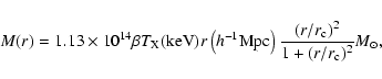
For a single thin lens, such as a cluster of galaxies, the strength of the
lens is expressed in the dimensionless mass surface density ![]() ,
where
,
where
 |
(1) |
 |
(2) |
![\begin{figure}
\par\includegraphics[width=8.8cm,clip]{H4502F1.ps}
\end{figure}](/articles/aa/full/2003/39/aah4502/img25.gif) |
Figure 1:
Plotted above are the values of
|
| Open with DEXTER | |
Table 1: Summary of cluster data.
What is measured from the background galaxies, however, is not ![]() ,
but
the reduced shear g, which is related to the gravitational shear
,
but
the reduced shear g, which is related to the gravitational shear ![]() by
by
 |
(3) |
 |
(5) |
 |
(6) |
A similar equation can be calculated for the non-weak lensing case,
when
![]() ,
however in
this case the effective mean lensing redshift will be a function of the
local mass surface density. Further, due to the competing effects of
deflection and
magnification of the background galaxies, the redshift distribution of a
magnitude limited sample of the background galaxies will change with
increasing
,
however in
this case the effective mean lensing redshift will be a function of the
local mass surface density. Further, due to the competing effects of
deflection and
magnification of the background galaxies, the redshift distribution of a
magnitude limited sample of the background galaxies will change with
increasing ![]() (e.g. Dye et al. 2001). As a result, accurately comparing
the mean lensing redshifts of two galaxy populations near the cores of massive
clusters is much harder than at large distances from the cores, and is near
impossible without some pre-existing knowledge of the mass distribution of
the clusters.
(e.g. Dye et al. 2001). As a result, accurately comparing
the mean lensing redshifts of two galaxy populations near the cores of massive
clusters is much harder than at large distances from the cores, and is near
impossible without some pre-existing knowledge of the mass distribution of
the clusters.
As can be seen in Eq. (4), in the weak lensing limit a sheet of constant
density across the field can be added to the cluster surface density without
affecting the measured shear. As a result, one cannot determine ![]() or
or
![]() at a given point uniquely, but can only determine them to
within an unknown additive constant. As a result, a useful statistic to
use as a mass estimate is aperture densitometry (Fahlman et al. 1994; Clowe et al. 2000),
at a given point uniquely, but can only determine them to
within an unknown additive constant. As a result, a useful statistic to
use as a mass estimate is aperture densitometry (Fahlman et al. 1994; Clowe et al. 2000),
Further, in the non-weak lensing limit,
![]() in aperture densitometry is replaced by
in aperture densitometry is replaced by ![]() ,
and the resulting
statistic is no longer measuring
,
and the resulting
statistic is no longer measuring
![]() .
The statistic is also no longer linear
with
.
The statistic is also no longer linear
with
![]() ,
but can still be used to find a best
fit
,
but can still be used to find a best
fit
![]() by converting a mass profile, which must
cover the same range in r as
by converting a mass profile, which must
cover the same range in r as
![]() ,
to a reduced
shear profile and calculating the resulting
,
to a reduced
shear profile and calculating the resulting
![]() statistic to compare with the measured value.
If, however, one does have a mass profile determined from an independent data
set, one will typically get a higher signal-to-noise measurement by fitting
the observed reduced shear profile directly with the mass profile converted
to reduced shear profile via the
statistic to compare with the measured value.
If, however, one does have a mass profile determined from an independent data
set, one will typically get a higher signal-to-noise measurement by fitting
the observed reduced shear profile directly with the mass profile converted
to reduced shear profile via the
![]() fit parameter. In both
cases, the fitting for the mean lensing redshift can only be done in regions
with a sufficiently low
fit parameter. In both
cases, the fitting for the mean lensing redshift can only be done in regions
with a sufficiently low ![]() and
and ![]() that the magnification and
displacement of the background galaxies do not significantly alter the
background galaxy redshift distribution.
that the magnification and
displacement of the background galaxies do not significantly alter the
background galaxy redshift distribution.
![\begin{figure}
\par\includegraphics[width=17cm,clip]{H4502F2.ps}
\end{figure}](/articles/aa/full/2003/39/aah4502/img84.gif) |
Figure 2:
Shown above are the best fit values for the mean lensing redshift
of the background galaxy population as a function of
|
| Open with DEXTER | |
The standard model used to fit the X-ray data of the clusters is the
![]() -model, for which the mass enclosed in a sphere of radius r is
-model, for which the mass enclosed in a sphere of radius r is
 |
(8) |
| |
= | 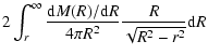 |
|
| = | 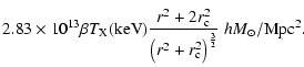 |
(9) |
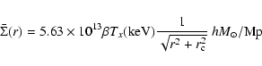 |
(10) |
In the above comparison, all of the background galaxies were de-magnified
before applying magnitude cuts to the catalog
by the amount
![]() by assuming that
by assuming that
![]() ,
and using
the best fit
,
and using
the best fit
![]() model to the measured reduced shear over
a
model to the measured reduced shear over
a
![]() range to calculate
range to calculate
![]() .
This is a first order correction to the magnification of the
observed background galaxy population, and thus should make the observed
population be on average the same as those observed in blank fields.
However, because the lensing strength, and thus the magnification, is
a function of the redshift of the galaxies, the average magnification which
we corrected for will be slightly too low for high redshift galaxies and
too high for low redshift galaxies. Thus, higher redshift galaxies will
still be slightly magnified and lower redshift galaxies will be slightly
de-magnified. This will result in
a slight overestimation of
.
This is a first order correction to the magnification of the
observed background galaxy population, and thus should make the observed
population be on average the same as those observed in blank fields.
However, because the lensing strength, and thus the magnification, is
a function of the redshift of the galaxies, the average magnification which
we corrected for will be slightly too low for high redshift galaxies and
too high for low redshift galaxies. Thus, higher redshift galaxies will
still be slightly magnified and lower redshift galaxies will be slightly
de-magnified. This will result in
a slight overestimation of
![]() by this method, but
from simulations we have determined this systematic error is an order of
magnitude below the random errors in the measurement. In future, larger
data-sets, this error could be minimized by binning the data by colors into
groups with similar redshifts.
by this method, but
from simulations we have determined this systematic error is an order of
magnitude below the random errors in the measurement. In future, larger
data-sets, this error could be minimized by binning the data by colors into
groups with similar redshifts.
![\begin{figure}
\par\includegraphics[width=8.8cm,clip]{H4502F3.ps}
\end{figure}](/articles/aa/full/2003/39/aah4502/img96.gif) |
Figure 3:
Shown above are the best fit values for
|
| Open with DEXTER | |
As can be seen in Fig. 2, if the ![]() -model of the X-ray clusters is
extrapolated to determine the mean
-model of the X-ray clusters is
extrapolated to determine the mean ![]() in the annular region subtracted
in
in the annular region subtracted
in
![]() ,
the allowable value for
,
the allowable value for
![]() is
in good agreement with that calculated from photometric redshifts of galaxies
with the same magnitude and color range in the HDF-S (Fontana et al. 1999).
If one is going to extrapolate the X-ray model over the region containing
the measured reduced shear, however, one will obtain both a better
signal-to-noise and avoid the systematic error of assuming g is
is
in good agreement with that calculated from photometric redshifts of galaxies
with the same magnitude and color range in the HDF-S (Fontana et al. 1999).
If one is going to extrapolate the X-ray model over the region containing
the measured reduced shear, however, one will obtain both a better
signal-to-noise and avoid the systematic error of assuming g is ![]() by fitting the reduced shear profile with the
by fitting the reduced shear profile with the ![]() -model surface mass profile.
In Fig. 3 are the best fit values of
-model surface mass profile.
In Fig. 3 are the best fit values of
![]() when fitting
the shear and mass models over a
when fitting
the shear and mass models over a
![]() range. The
300 h-1 kpc inner radius was chosen to avoid the large
changes to the background galaxy redshift distribution which occurs
due to the larger magnifications and displacements of the background galaxies
near the cluster core.
range. The
300 h-1 kpc inner radius was chosen to avoid the large
changes to the background galaxy redshift distribution which occurs
due to the larger magnifications and displacements of the background galaxies
near the cluster core.
For these fits, the ![]() -model was converted from
-model was converted from ![]() to
to ![]() by the fit value
by the fit value
![]() ,
and used to
calculate
the reduced shear profile
,
and used to
calculate
the reduced shear profile
![]() .
The model's
.
The model's
![]() and
and
![]() profiles were then used to calculate and correct for
the average magnification for each background galaxy as a function of
distance from the cluster center. The magnitude corrected
catalog then had the magnitude and color cuts applied to select the catalog
used to measure the reduced shear. The measured reduced shear was then
compared with the model using a
profiles were then used to calculate and correct for
the average magnification for each background galaxy as a function of
distance from the cluster center. The magnitude corrected
catalog then had the magnitude and color cuts applied to select the catalog
used to measure the reduced shear. The measured reduced shear was then
compared with the model using a ![]() statistic, which was minimized
to find the best fit
statistic, which was minimized
to find the best fit
![]() .
The resulting
.
The resulting
![]() measurements can then be converted to
a
measurements can then be converted to
a
![]() for each cluster. For a broad background galaxy
redshift distribution, the resulting
for each cluster. For a broad background galaxy
redshift distribution, the resulting
![]() is a function
of the lensing cluster redshift due to the change in the
is a function
of the lensing cluster redshift due to the change in the
![]() with cluster
redshift. The results are in good agreement
with the photometric redshift distribution of faint galaxies from the HDF-S.
with cluster
redshift. The results are in good agreement
with the photometric redshift distribution of faint galaxies from the HDF-S.
It should be noted that the mean lensing background galaxy redshift is a function of magnitude, color, size, and surface brightness cuts placed on the background galaxy catalog. Because the images for the five clusters used in this comparison are similar in exposure times and seeing, the weak lensing results all use the same background galaxy redshift distribution. In general, however, this will not be the case and the mean lensing redshifts as a function of cluster redshift shown in Fig. 3 will not be the mean lensing redshifts of the observations. For each observation, the mean lensing redshift would need to be computed from a redshift catalog by applying the same cuts as are used to select the background galaxies.
As was discussed in Sect. 2, for a high-redshift lens, the strength of the
shear acting on a background galaxy greatly depends on the angular distance of the
background galaxy. As the ellipticity induced in the galaxy by the
weak lensing shear is smaller than the typical intrinsic ellipticity of the
galaxy, one cannot use this to determine angular distances of individual galaxies.
One can, however, use this to measure the relative distances of two galaxy
samples provided each sample has enough galaxies to reduce the mean
intrinsic ellipticity of the sample well below the expected shear level.
Ideally one would choose the samples in some manner, such as by using
photometric redshifts, which would allow the galaxies inside each sample
to be at a similar distance. It is, however, still
possible to measure a mean angular distance ratio for two sets of galaxies,
each of which has a broad redshift distribution.
![\begin{figure}
\par\includegraphics[width=8.8cm,clip]{H4502F4.ps}
\end{figure}](/articles/aa/full/2003/39/aah4502/img102.gif) |
Figure 4:
Shown above are values for the mean shear for the background galaxies,
divided into four magnitude bins (23-24, 24-25, 25-25.7, and 25.7-26.3),
relative to the mean shear of the brightest magnitude bin. Only galaxies
located further than
350 h-1 kpc from the cluster centers were used
to compute the mean shear.
The mean shear of the three
|
| Open with DEXTER | |
In the weak lensing limit, where
![]() ,
the shear acting upon a
galaxy is a function of the lens mass, the galaxy position, the lens and
galaxy redshifts, and the cosmological model. If the galaxy samples
being compared have the same spatial distribution about a common lens, then
the ratio of the mean shears is a function only of the redshift of the lens,
the redshift distributions of the samples, and the cosmological model.
If the magnification of the background galaxies is corrected for, the galaxy
samples around different lenses of similar redshift can be coadded to improve
the signal-to-noise of the mean shear ratio.
,
the shear acting upon a
galaxy is a function of the lens mass, the galaxy position, the lens and
galaxy redshifts, and the cosmological model. If the galaxy samples
being compared have the same spatial distribution about a common lens, then
the ratio of the mean shears is a function only of the redshift of the lens,
the redshift distributions of the samples, and the cosmological model.
If the magnification of the background galaxies is corrected for, the galaxy
samples around different lenses of similar redshift can be coadded to improve
the signal-to-noise of the mean shear ratio.
In Fig. 4 we show the relative strength of the mean shear signal for the
three ![]() clusters and the three
clusters and the three
![]() clusters in four
magnitude bins. For both sets of clusters, the strength of the shear signal
increases with increasing magnitude, with significances, calculated from
Student's t-distribution, of 96.4%, 72.4%, and 96.0% for the
clusters in four
magnitude bins. For both sets of clusters, the strength of the shear signal
increases with increasing magnitude, with significances, calculated from
Student's t-distribution, of 96.4%, 72.4%, and 96.0% for the
![]() clusters,
clusters, ![]() clusters, and both sets combined
respectively. This is consistent with the mean redshift
of the background galaxies increasing with magnitude. Also shown in
Fig. 4 are the shears which would be measured from the Fontana
HDF-S photometric redshifts when using the same magnitude bins.
clusters, and both sets combined
respectively. This is consistent with the mean redshift
of the background galaxies increasing with magnitude. Also shown in
Fig. 4 are the shears which would be measured from the Fontana
HDF-S photometric redshifts when using the same magnitude bins.
Due to
![]() increasing more rapidly for higher
redshift lenses, one should, in theory, be able to use multiple lenses at
different redshifts to obtain estimates for the redshift distribution of the
background galaxies. This can be seen in Fig. 4 in which the difference
in the lensing strength predicted by the HDF-S photometric redshift catalogs
for the
increasing more rapidly for higher
redshift lenses, one should, in theory, be able to use multiple lenses at
different redshifts to obtain estimates for the redshift distribution of the
background galaxies. This can be seen in Fig. 4 in which the difference
in the lensing strength predicted by the HDF-S photometric redshift catalogs
for the ![]() and
and
![]() lenses continues to increase with
increasing magnitude of the background galaxies. This difference, however,
is too small to measure with this data set. We estimate that we would need
a data set ten times as large (60 clusters) with the same quality of data
in order to successfully apply any of the techniques (e.g. Bartelmann & Narayan 1995) to measure the background galaxy redshift distribution.
lenses continues to increase with
increasing magnitude of the background galaxies. This difference, however,
is too small to measure with this data set. We estimate that we would need
a data set ten times as large (60 clusters) with the same quality of data
in order to successfully apply any of the techniques (e.g. Bartelmann & Narayan 1995) to measure the background galaxy redshift distribution.
One source of systematic error in the weak lensing mass estimates can be
the dilution of the shear signal from blue cluster dwarf galaxies. The
background galaxy catalogs were selected from all detected galaxies with
23<R<26.3 and R-I<0.9. The color selection removed the red-sequence
of cluster ellipticals from the galaxy catalogs, but would have left some
fraction of the bluer cluster galaxies. Cluster galaxies at ![]() are redder in R-I than those at
are redder in R-I than those at ![]() .
As a result, applying the
same color cut to both sets of clusters would remove a greater fraction of
cluster spirals from the
.
As a result, applying the
same color cut to both sets of clusters would remove a greater fraction of
cluster spirals from the ![]() background galaxy catalogs than from the
background galaxy catalogs than from the
![]() catalogs. From number counts of dwarf galaxies in nearby clusters
(e.g. Trentham 1998), we estimate that the weak lensing shear signal, and thus
the derived masses, could be under-predicted by 10-20% for the
catalogs. From number counts of dwarf galaxies in nearby clusters
(e.g. Trentham 1998), we estimate that the weak lensing shear signal, and thus
the derived masses, could be under-predicted by 10-20% for the ![]() clusters. This estimate, however, depends greatly on a lack of evolution in
the number counts of dwarf galaxies compared to the cluster L* population.
clusters. This estimate, however, depends greatly on a lack of evolution in
the number counts of dwarf galaxies compared to the cluster L* population.
We also compared the ratio of the shear signals as a function of magnitude, and demonstrate that the measured shear does tend to increase with increasing magnitude. The amount of the increase is again in good agreement with the photometric redshifts of the HDF-S. This result is also in agreement withthat of Hoekstra et al. (2000), who compared the relative lensing strength of galaxies in an HST mosaic of MS 1054.4-0321. The level of noise in our comparison, however, is too great to attempt to obtain a meaningful mean lensing redshift as a function of magnitude for the background galaxies.
Acknowledgements
We thank Gillian Wilson, Lev Koffman, Len Cowie, Dave Sanders, John Learned, and Peter Schneider for their help and advice. We also wish to thank Megan Donahue, Isabella Gioia, and J. Patrick Henry for sharing their X-ray data with us. This work was supported by NSF Grants AST-9529274 and AST-9500515, Nasa Grant NAG5-2594, ASI-CNR, and the Deutsche Forschungsgemeinschaft under the project SCHN 342/3-1.