All Figures

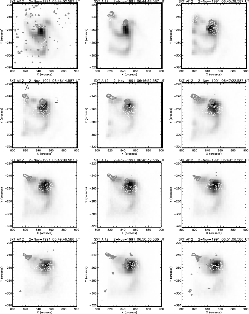
$\begin{figure} \par\resizebox{16.1cm}{!}{\includegraphics{4109.f1.ps}}\end{figure}$ Figure 1: A series of images of the flare of 2 November 1991 in the Al12 filter of the SXT. Overlaid are contours of the WL emission (solid lines) and of the M1 channel (dashed white lines). There are two WLF kernels that correlate well spatially with the M1 sources, with a small offset. The larger of the two sources centred at (850, -260) is also the stronger of the two and the longest lived. The northern source seems to correspond to a footpoint.
Open with DEXTER

In the text

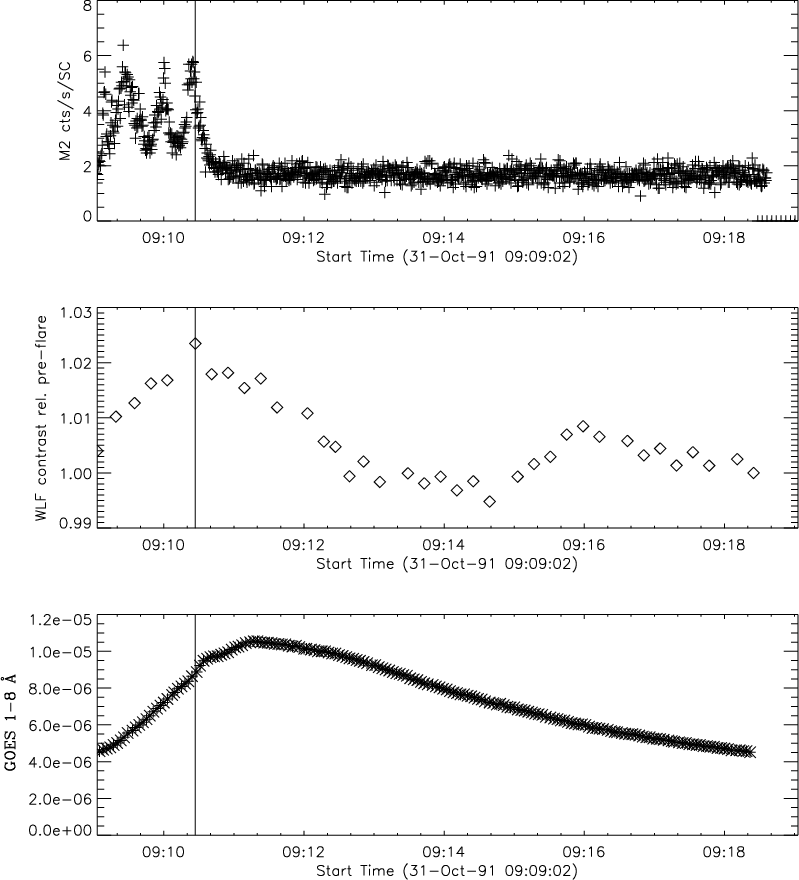
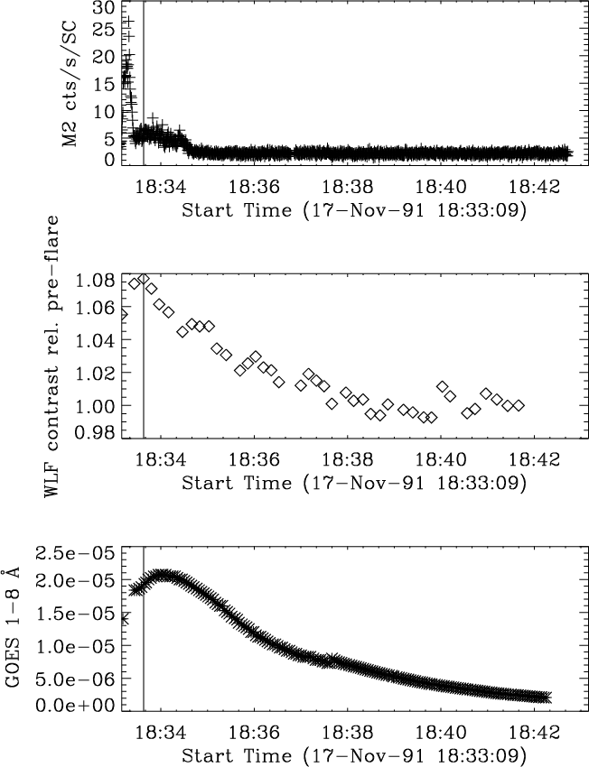
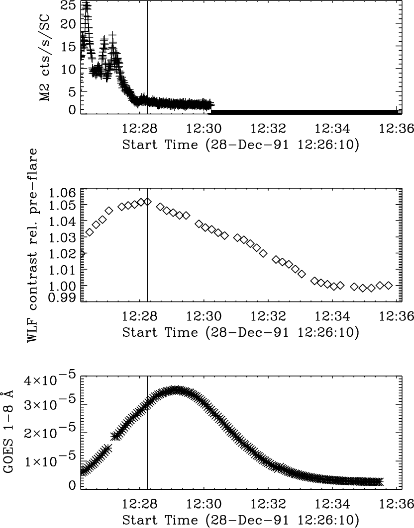
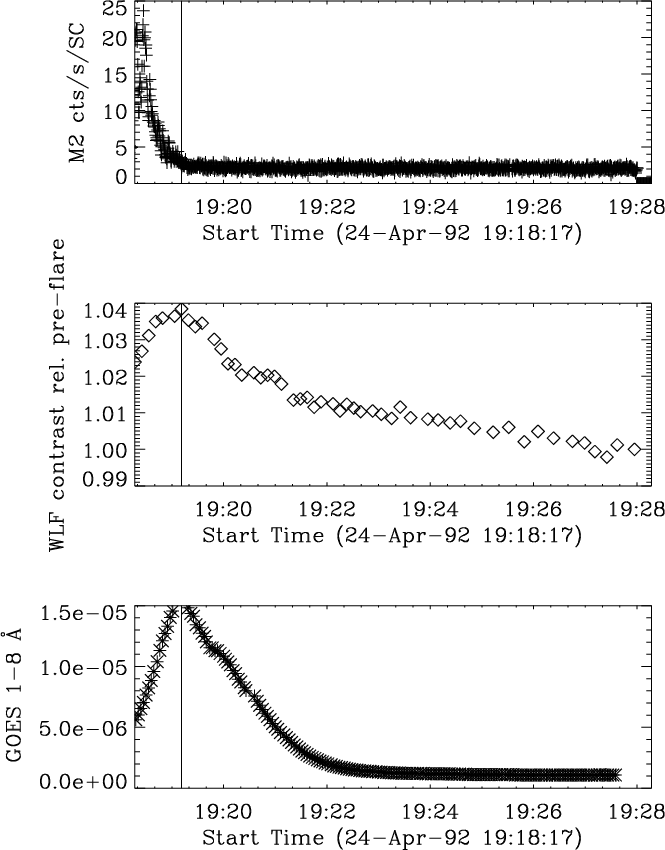
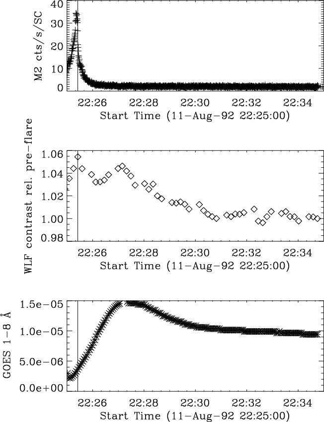
$\begin{figure} \par\resizebox{\hsize}{!}{\includegraphics{4109.f2.ps}}\end{figure}$ Figure 2: Time series plots of the 2 November 1991 flare. Top panel: M2 cts/s/SC. Middle panel: WLF contrast calculated relative to the pre-flare brightness in the location that the flare occurred. Lower panel: GOES 1-8 Å flux. The vertical line indicates the time of maximum WLF contrast.
Open with DEXTER

In the text

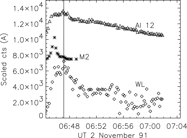$\begin{figure} \par\resizebox{8.5cm}{!}{\includegraphics{4109.f3.ps}}\end{figure}$ Figure 3: Light-curves of the WLF, M2 and Al12 emission in the northern most kernel A of the flare of 2 November 1991, centred on (820, -235). The Al12 and M2 curves have been scaled and shifted relative to the WLF curve for clarity. In this instance WLF cts are from the difference cube (DN/s). The vertical line marks the time of peak WLF cts in this kernel.
Open with DEXTER

In the text

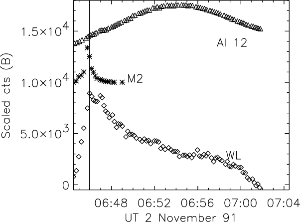$\begin{figure} \par\resizebox{8.5cm}{!}{\includegraphics{4109.f4.ps}}\end{figure}$ Figure 4: Light-curves of the WLF, M2 and Al12 emission in kernel B of the flare of 2 November 1991 centred on (850, -260). The Al12 and M2 curves have been scaled and shifted relative to the WLF curve for clarity. In this instance WLF cts are from the difference cube (DN/s). The vertical line marks the time of peak WLF cts in this kernel.
Open with DEXTER

In the text

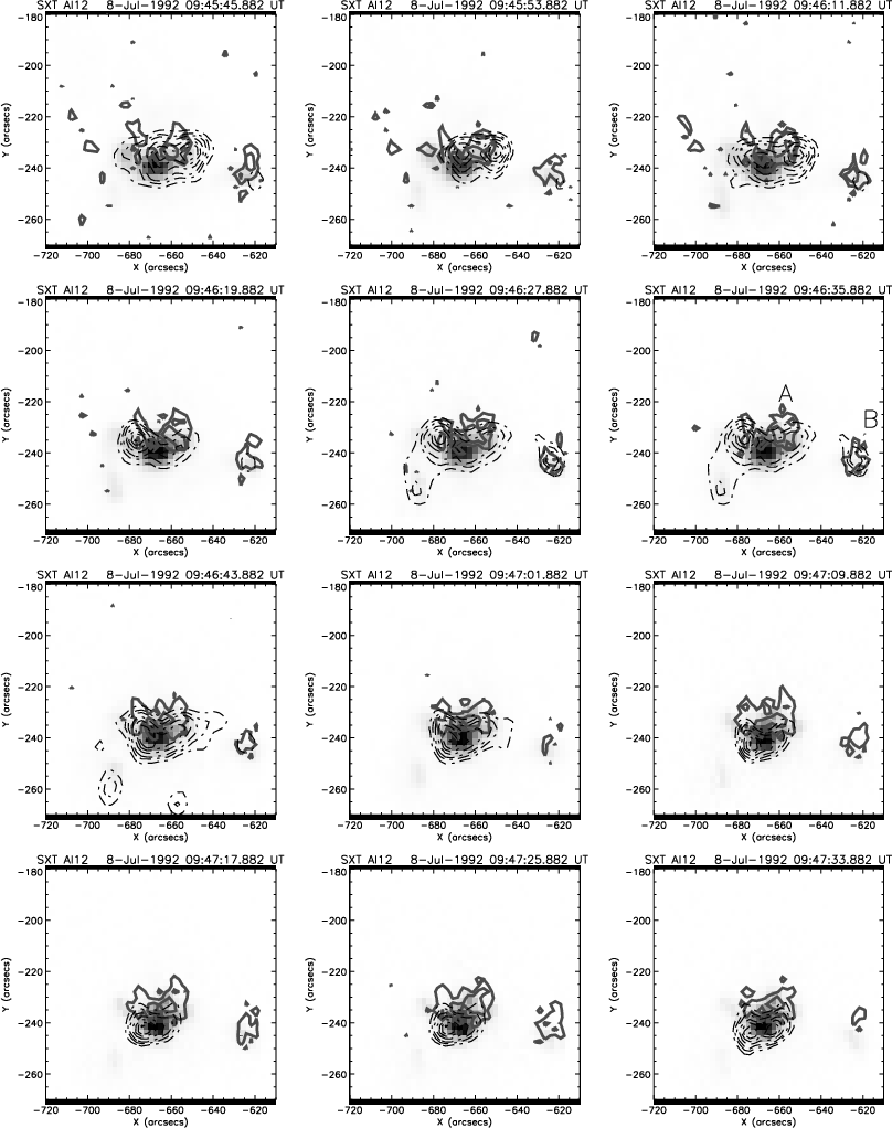$\begin{figure} \par\resizebox{15.8cm}{!}{\includegraphics{4109.f5.ps}}\end{figure}$ Figure 5: A series of images of the flare of 8 July 1992 in the Al12 filter of the SXT. Overlaid are contours of the WL emission (solid lines) and of the M2 channel (dashed black line). WLF kernel A at (-665, -235) correlates well spatially with the M2 source at this location. Both the WLF and the M2 emission in this location give the impression of a double footpoint structure. In addition there is a second WLF source, B, at (-620, -240) which also correlates well with M2 emission in this location.
Open with DEXTER

In the text

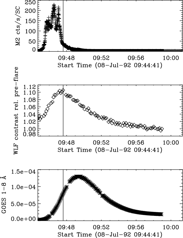$\begin{figure} \par\resizebox{8.4cm}{!}{\includegraphics{4109.f6.ps}}\end{figure}$ Figure 6: Time series plots of the 8 July 1992 flare. Top panel: M2 cts/s/SC. Middle panel: WLF contrast calculated relative to the pre-flare brightness in the location that the flare occurred. Lower panel: GOES 1-8 Å flux. The vertical line indicates the time of maximum WLF contrast.
Open with DEXTER

In the text

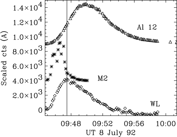$\begin{figure} \par\resizebox{8.2cm}{!}{\includegraphics{4109.f7.ps}}\end{figure}$ Figure 7: Light-curves of the WLF, M2 and Al12 emission in source A for the 8 July 1992 flare centred at (-665, -235). The Al12 and M2 curves have been scaled and shifted relative to the WLF curve for clarity. In this instance WLF cts are from the difference cube (DN/s).
Open with DEXTER

In the text

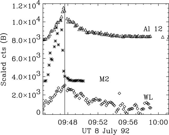$\begin{figure} \par\resizebox{8.3cm}{!}{\includegraphics{4109.f8.ps}}\end{figure}$ Figure 8: Light-curves of the WLF, M2 and Al12 emission in source B for the 8 July 1992 flare centred at (-620, -240). The Al12 and M2 curves have been scaled and shifted relative to the WLF curve for clarity. In this instance WLF cts are from the difference cube (DN/s).
Open with DEXTER

In the text

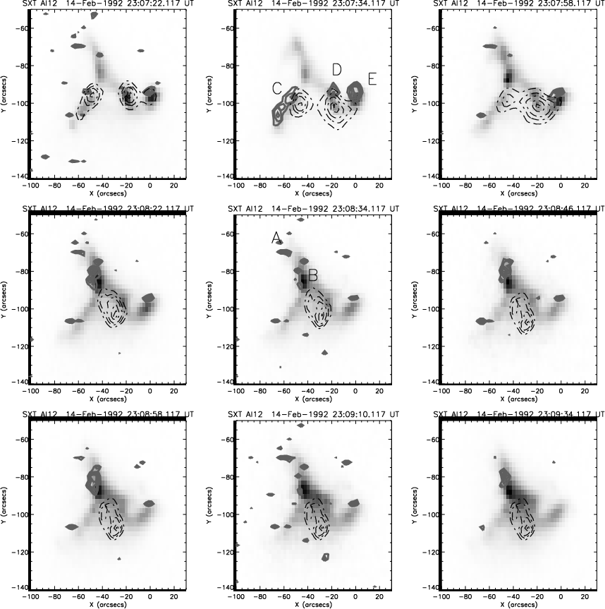$\begin{figure} \par\resizebox{15.9cm}{!}{\includegraphics{4109.f9.ps}}\end{figure}$ Figure 9: A series of images of the flare of 14 February 1992 in the Al12 filter of the SXT. Overlaid are contours of the WL emission (solid lines) and of the M1 channel (dashed black line). There are 5 WLF kernels, 4 of which correlate well spatially with the M1 sources during the impulsive phase of the flare.
Open with DEXTER

In the text

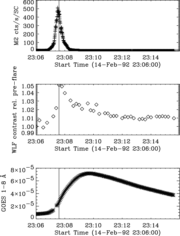$\begin{figure} \par\resizebox{8.5cm}{!}{\includegraphics{4109.f10.ps}}\end{figure}$ Figure 10: Time series plots of the 14 February 1992 flare. Top panel: M2 cts/s/SC. Middle panel: WLF contrast calculated relative to the pre-flare brightness in the location that the flare occurred. Lower panel: GOES 1-8 Å flux. The vertical line indicates the time of maximum WLF contrast.
Open with DEXTER

In the text

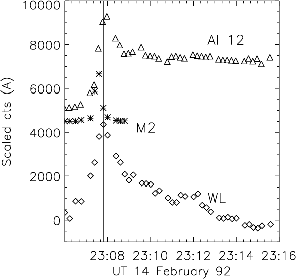$\begin{figure} \par\resizebox{8.3cm}{!}{\includegraphics{4109.f11.ps}}\end{figure}$ Figure 11: Light-curves of the WLF, M2 and Al12 emission in the northern most kernel (A) of the flare of 14 February 1992, centred on (-60, -70). The Al12 and M2 curves have been scaled and shifted relative to the WLF curve for clarity. In this instance WLF cts are from the difference cube (DN/s).
Open with DEXTER

In the text

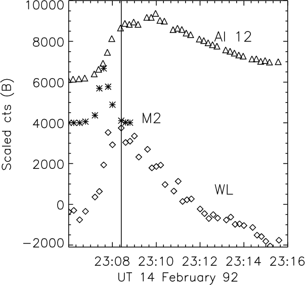$\begin{figure} \par\resizebox{8.5cm}{!}{\includegraphics{4109.f12.ps}}\end{figure}$ Figure 12: Light-curves of the WLF, M2 and Al12 emission in kernel B of the flare of 14 February 1992, centred on (-50, -85). The Al12 and M2 curves have been scaled and shifted relative to the WLF curve for clarity. In this instance WLF cts are from the difference cube (DN/s).
Open with DEXTER

In the text

$\begin{figure} \par\resizebox{8.7cm}{!}{\includegraphics{4109.f13.ps}}\end{figure}$ Figure 13: Light-curves of the WLF, M2 and Al12 emission in kernel C of the flare of 14 February 1992, centred on (-55, -95). The Al12 and M2 curves have been scaled and shifted relative to the WLF curve for clarity. In this instance WLF cts are from the difference cube (DN/s).
Open with DEXTER

In the text

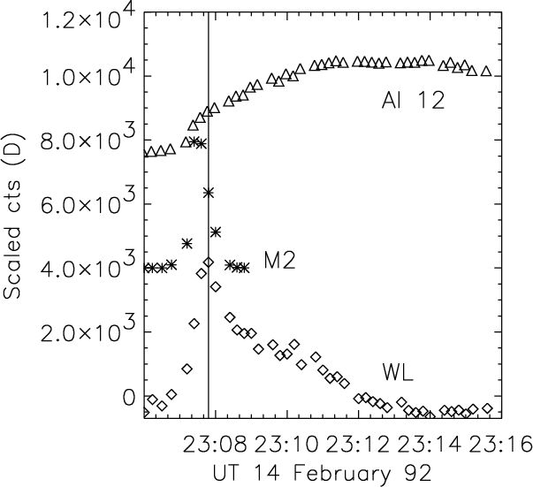$\begin{figure} \par\resizebox{8.5cm}{!}{\includegraphics{4109.f14.ps}}\end{figure}$ Figure 14: Light-curves of the WLF, M2 and Al12 emission in kernel D of the flare of 14 February 1992, centred on (-20, -95). The Al12 and M2 curves have been scaled and shifted relative to the WLF curve for clarity. In this instance WLF cts are from the difference cube (DN/s).
Open with DEXTER

In the text

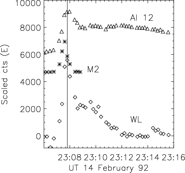$\begin{figure} \par\resizebox{8.3cm}{!}{\includegraphics{4109.f15.ps}}\end{figure}$ Figure 15: Light-curves of the WLF, M2 and Al12 emission in the northern most kernel E of the flare of 14 February 1992, centred on (0, -95). The Al12 and M2 curves have been scaled and shifted relative to the WLF curve for clarity. In this instance WLF cts are from the difference cube (DN/s).
Open with DEXTER

In the text

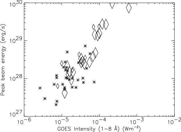$\begin{figure} \par\resizebox{8.3cm}{!}{\includegraphics{4109.f16.ps}}\end{figure}$ Figure 16: Scatter plot showing the relationship between peak GOES flux in the 1-8 Å channel and the peak electron beam power calculated for a thick target assumption and a low energy cut-off of 20 keV. * represents the non-WLFs and $\diamond$ represents the WLFs, with larger symbol size corresponding to those events that showed WLF contrast $\geq$ 5% relative to the pre-flare continuum intensity in the flare region.
Open with DEXTER

In the text

$\begin{figure} \par\resizebox{15.5cm}{!}{\includegraphics{4109.f17.ps}}\end{figure}$ Figure 17: Histogram showing the distribution of electron beam power for non-WLFs, WLFs with peak contrast <5% and WLFs with peak contrast >5%.
Open with DEXTER

In the text

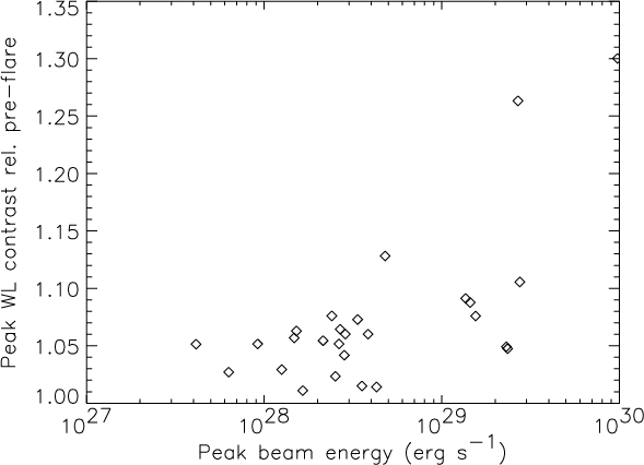$\begin{figure} \par\resizebox{8.3cm}{!}{\includegraphics{4109.f18.ps}}\end{figure}$ Figure 18: Scatter plot showing the relationship between the peak electron beam power calculated for a thick target assumption and a low energy cut-off of 20 keV and the maximum WLF contrast relative to the pre-flare continuum intensity in the flare region.
Open with DEXTER

In the text

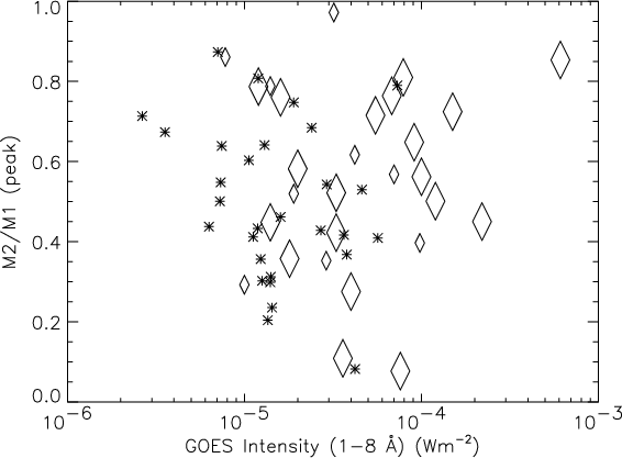$\begin{figure} \par\resizebox{8cm}{!}{\includegraphics{4109.f19.ps}}\end{figure}$ Figure 19: Scatter plot showing the relationship between the peak GOES flux in the 1-8 Å channel and the peak value of M2/M1 for both non-WLFs and WLFs. * represents the non-WLFs and $\diamond$ represents the WLFs, with larger symbol size corresponding to those events that showed WLF contrast $\geq$ 5% relative to the pre-flare continuum intensity in the flare region.
Open with DEXTER

In the text

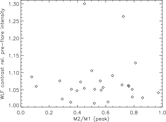$\begin{figure} \par\resizebox{8cm}{!}{\includegraphics{4109.f20.ps}}\end{figure}$ Figure 20: Scatter plot showing the relationship between the peak value of M2/M1 and the peak WLF contrast relative to the pre-flare continuum intensity in the flare region. Here * represents the non-WLFs and $\diamond$ represents the WLFs.
Open with DEXTER

In the text

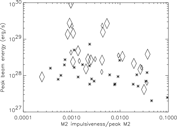$\begin{figure} \par\resizebox{8.5cm}{!}{\includegraphics{4109.f21.ps}}\end{figure}$ Figure 21: Scatter plot showing the relationship between the impulsiveness of the M2 emission, determined as described in the text, and the peak beam energy calculated for a thick target assumption and a low energy cut-off of 20 keV. * represents the non-WLFs and $\diamond$ represents the WLFs, with larger symbol size corresponding to those events that showed WLF contrast $\geq$ 5% relative to the pre-flare continuum intensity in the flare region.
Open with DEXTER

In the text

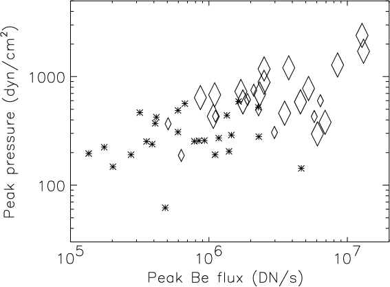$\begin{figure} \par\resizebox{8cm}{!}{\includegraphics{4109.f22.ps}}\end{figure}$ Figure 22: Scatter plot showing peak coronal pressure against peak Be 119 flux. * represents non-WLFs, and $\diamond$ represents WLFs.
Open with DEXTER

In the text

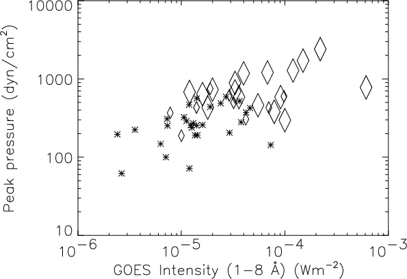$\begin{figure} \par\resizebox{8.4cm}{!}{\includegraphics{4109.f23.ps}}\end{figure}$ Figure 23: Scatter plot showing peak coronal pressure against peak GOES intensity. * represents non-WLFs, and $\diamond$ represents WLFs, with larger symbols representing higher contrast. Note that the flare with largest GOES flux was the 27 October 91 event, which was poorly observed preventing us from accurately deriving the contrast.
Open with DEXTER

In the text

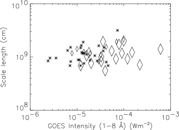$\begin{figure} \par\resizebox{8.2cm}{!}{\includegraphics{4109.f24.ps}}\end{figure}$ Figure 24: Scatter plot showing SXR scale length = $\sqrt {area > FWHM}$ against peak GOES intensity. Here * represents non-WLFs, and $\diamond$ represents WLFs. Note that the flare with largest GOES flux was the27 October 91 event, which was poorly observed preventing us from accurately deriving the contrast.
Open with DEXTER

In the text

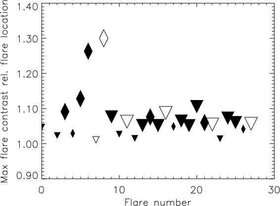$\begin{figure} \par\resizebox{8cm}{!}{\includegraphics{4109.f25.ps}}\end{figure}$ Figure 25: Scatter plot showing the peak WLF contrast relative to the pre-flare continuum intensity in the flare region. $\diamond$ represents those WLFs that showed associated $\gamma$ -ray emission, while $\bigtriangledown$ represents those events with no associated $\gamma$ -rays. Filled symbols indicate a location on the solar disk, while open symbols indicated events that occurred on the limb. Larger symbol size indicates $\geq$ 5% peak contrast. Flare number is given in Table 1.
Open with DEXTER

In the text

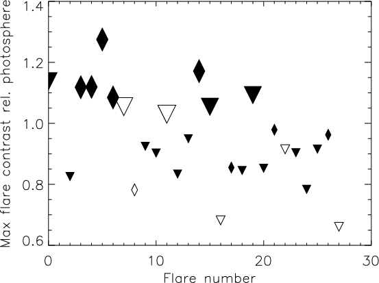$\begin{figure} \par\resizebox{7.8cm}{!}{\includegraphics{4109.f26.ps}}\end{figure}$ Figure 26: Scatter plot showing the peak WLF contrast relative to the neighbouring quiet photospheric continuum intensity. $\diamond$ represents those WLFs that showed associated $\gamma$ -ray emission, while $\bigtriangledown$ represents those events with no associated $\gamma$ -rays. Filled symbols indicate a location on the solar disk, while open symbols indicated events that occurred on the limb. Larger symbol size indicates $\geq$ 0.5% peak contrast. Flare number is given in Table 1.
Open with DEXTER

In the text

$\begin{figure} \par\includegraphics[width=8.8cm]{4109on.f1.ps} \end{figure}$ Figure A.1: Time series plots of the 24 October 1991 flare. Top panel: M2 cts/s/SC. Middle panel: WLF contrast calculated relative to the pre-flare brightness in the location that the flare occurred. Lower panel: GOES 1-8 Å flux. The vertical line indicates the time of maximum WLF contrast.

In the text

$\begin{figure} \par\includegraphics[width=8.8cm]{4109on.f2.ps} % \end{figure}$ Figure A.2: Light-curves of the WLF, M2 and Al12 emission in kernel A of the flare of 24 October 1991 centred on (-660, -265). The Al12 and M2 curves have been scaled and shifted relative to the WLF curve for clarity. In this instance WLF cts are from the difference cube (DN/s). The vertical line marks the time of peak WLF cts in this kernel.

In the text

$\begin{figure} \par\includegraphics[width=8.8cm]{4109on.f3.ps} \def \@captype{figure}\end{figure}$ Figure A.3: Light-curves of the WLF, M2 and Al12 emission in kernel B of the flare of 24 October 1991 centred on (-675, -320). The Al12 and M2 curves have been scaled and shifted relative to the WLF curve for clarity. In this instance WLF cts are from the difference cube (DN/s). The vertical line marks the time of peak WLF cts in this kernel.

In the text

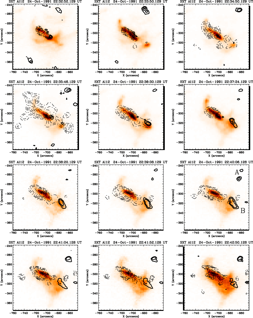$\begin{figure} \par\resizebox{16cm}{!}{\includegraphics{4109on.f4.ps}}\par\end{figure}$ Figure A.4: A series of images of the flare of 24 October 1991 in the Al12 filter of the SXT. Overlaid are contours of the WL emission (solid lines) and of the M1 channel (dashed lines).

In the text

$\begin{figure} \includegraphics[width=8.5cm]{4109on.f5.ps} \end{figure}$ Figure B.1: Time series plots of the 27 October 1991 flare. Top panel: M2 cts/s/SC. Middle panel: WLF contrast calculated relative to the pre-flare brightness in the location that the flare occurred. Lower panel: GOES 1-8 Å flux. The vertical line indicates the time of maximum WLF contrast.

In the text

$\begin{figure} \par\includegraphics[width=8.5cm]{4109on.f6.ps} \end{figure}$ Figure B.2: Light-curves of the WLF, M2 and Al12 emission in kernel A of the flare of 27 October 1991 centred on (-305, -310). The Al12 and M2 curves have been scaled and shifted relative to the WLF curve for clarity. In this instance WLF cts are from the difference cube (DN/s). The vertical line marks the time of peak WLF cts in this kernel.

In the text

$\begin{figure} \par\includegraphics[width=7.5cm]{4109on.f7.ps} \end{figure}$ Figure B.3: Light-curves of the WLF, M2 and Al12 emission in kernel B of the flare of 27 October 1991 centred on (-280, -295). The Al12 and M2 curves have been scaled and shifted relative to the WLF curve for clarity. In this instance WLF cts are from the difference cube (DN/s). The vertical line marks the time of peak WLF cts in this kernel.

In the text

$\begin{figure} \par\includegraphics[width=7.5cm]{4109on.f8.ps}\end{figure}$ Figure B.4: Light-curves of the WLF, M2 and Al12 emission in kernel C of the flare of 27 October 1991 centred on (-270, -270). The Al12 and M2 curves have been scaled and shifted relative to the WLF curve for clarity. In this instance WLF cts are from the difference cube (DN/s). The vertical line marks the time of peak WLF cts in this kernel.

In the text

$\begin{figure} \par\includegraphics[width=7.5cm]{4109on.f9.ps}\def \@captype{figure}\end{figure}$ Figure B.5: Light-curves of the WLF, M2 and Al12 emission in kernel D of the flare of 27 October 1991 centred on (-240, -280). The Al12 and M2 curves have been scaled and shifted relative to the WLF curve for clarity. In this instance WLF cts are from the difference cube (DN/s). The vertical line marks the time of peak WLF cts in this kernel.

In the text

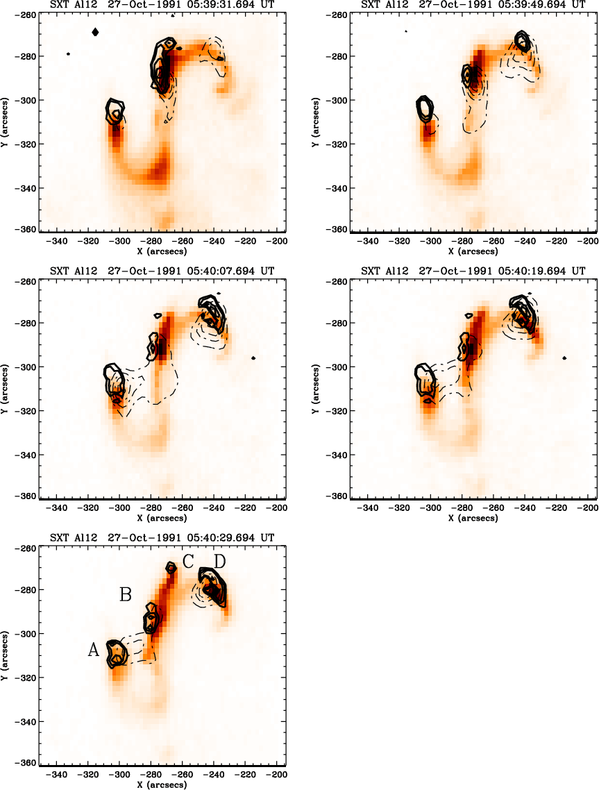$\begin{figure} \par\resizebox{16cm}{!}{\includegraphics{4109on.f10.ps}}\end{figure}$ Figure B.6: A series of images of the flare of 27 October 1991 in the Al12 filter of the SXT. Overlaid are contours of the WL emission (solid lines) and of the M1 channel (dashed lines).

In the text

$\begin{figure} \includegraphics{4109on.f11.ps}\end{figure}$ Figure C.1: Time series plots of the 31 October 1991 flare. Top panel: M2 cts/s/SC. Middle panel: WLF contrast calculated relative to the pre-flare brightness in the location that the flare occurred. Lower panel: GOES 1-8 Å flux. The vertical line indicates the time of maximum WLF contrast.

In the text

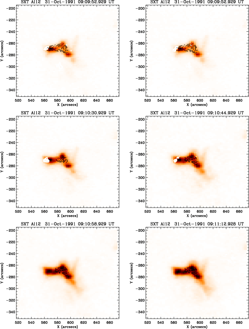$\begin{figure} \par\resizebox{16cm}{!}{\includegraphics{4109on.f12.ps}}\end{figure}$ Figure C.2: A series of images of the flare of 31 October 1991 in the Al12 filter of the SXT. Overlaid are contours of the WL emission (solid lines) and of the M1 channel (dashed lines).

In the text

$\begin{figure} \includegraphics[width=14cm,clip]{4109on.f13.ps}\end{figure}$ Figure D.1: Time series plots of the 9 November 1991 flare. Top panel: M2 cts/s/SC. Middle panel: WLF contrast calculated relative to the pre-flare brightness in the location that the flare occurred. Lower panel: GOES 1-8 Å flux. The vertical line indicates the time of maximum WLF contrast.

In the text

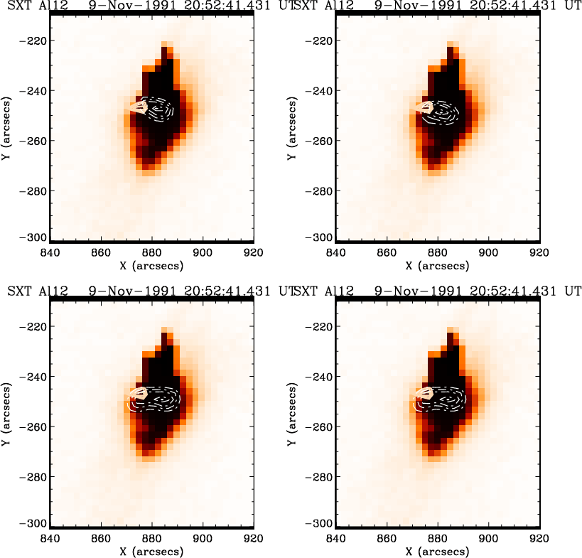$\begin{figure} \par\resizebox{16cm}{!}{\includegraphics{4109on.f14.ps}}\end{figure}$ Figure D.2: A series of images of the flare of 9 November 1991 in the Al12 filter of the SXT. Overlaid are contours of the WL emission (solid lines) and of the M1 channel (dashed lines).

In the text

$\begin{figure} \par\includegraphics[width=8cm]{4109on.f15.ps}\end{figure}$ Figure E.1: Time series plots of the 10 November 1991 flare. Top panel: M2 cts/s/SC. Middle panel: WLF contrast calculated relative to the pre-flare brightness in the location that the flare occurred. Lower panel: GOES 1-8 Å flux. The vertical line indicates the time of maximum WLF contrast.

In the text

$\begin{figure}\includegraphics[width=8cm]{4109on.f16.ps}\end{figure}$ Figure E.2: Light-curves of the WLF, M2 and Al12 emission in kernel A of the flare of 10 November 1991 centred on (-720, -230). The Al12 and M2 curves have been scaled and shifted relative to the WLF curve for clarity. In this instance WLF cts are from the difference cube (DN/s). The vertical line marks the time of peak WLF cts in this kernel.

In the text

$\begin{figure}\includegraphics[width=8cm]{4109on.f17.ps}\end{figure}$ Figure E.3: Light-curves of the WLF, M2 and Al12 emission in kernel B of the flare of 10 November 1991 centred on (-695, -265). The Al12 and M2 curves have been scaled and shifted relative to the WLF curve for clarity. In this instance WLF cts are from the difference cube (DN/s). The vertical line marks the time of peak WLF cts in this kernel.

In the text

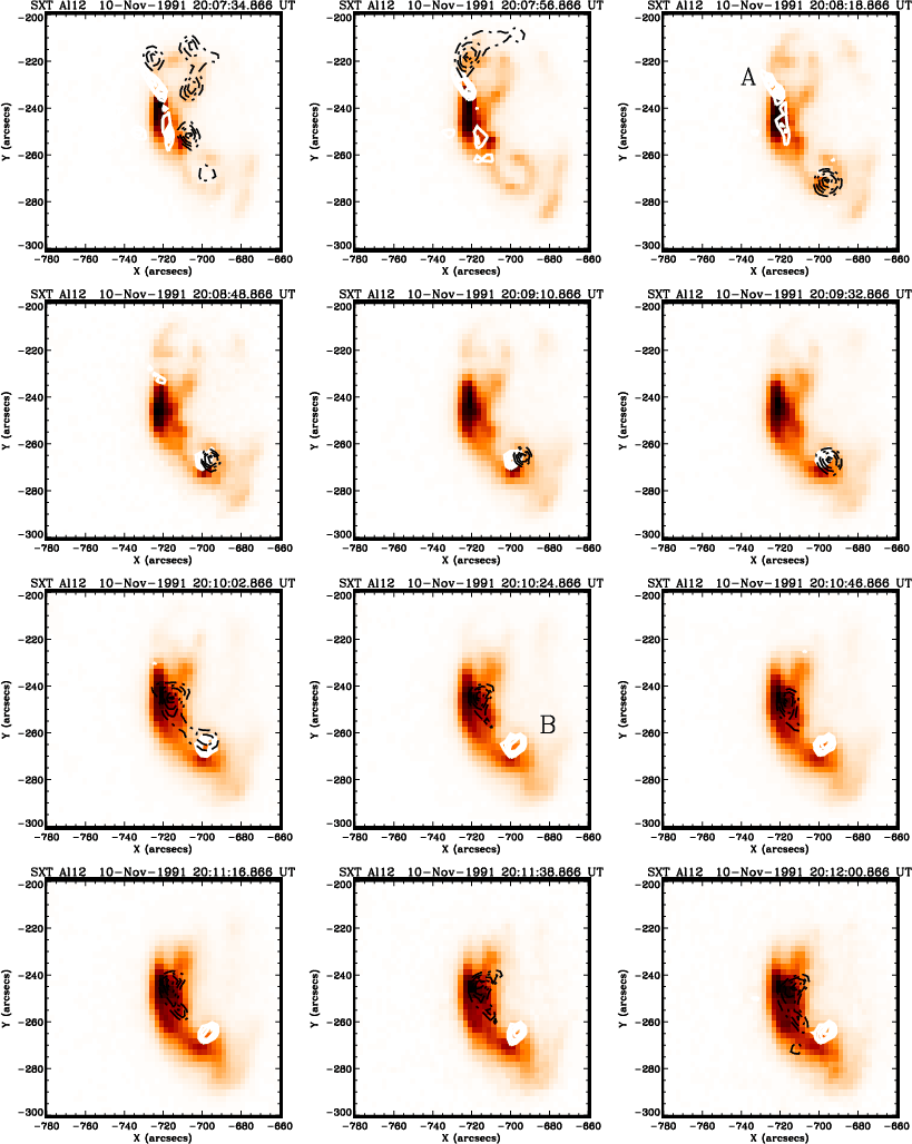$\begin{figure} \par\resizebox{16cm}{!}{\includegraphics{4109on.f18.ps}}\end{figure}$ Figure E.4: A series of images of the flare of 10 November 1991 in the Al12 filter of the SXT. Overlaid are contours of the WL emission (solid lines) and of the M1 channel (dashed lines).

In the text

$\begin{figure}\par\includegraphics[width=8cm]{4109on.f19.ps}\end{figure}$ Figure F.1: Time series plots of the 15 November 1991 flare. Top panel: M2 cts/s/SC. Middle panel: WLF contrast calculated relative to the pre-flare brightness in the location that the flare occurred. Lower panel: GOES 1-8 Å flux. The vertical line indicates the time of maximum WLF contrast.

In the text

$\begin{figure}\includegraphics[width=8cm]{4109on.f20.ps}\end{figure}$ Figure F.2: Light-curves of the WLF, M2 and Al12 emission in kernel A of the flare of 15 November 1991 centred on (300, -250). The Al12 and M2 curves have been scaled and shifted relative to the WLF curve for clarity. In this instance WLF cts are from the difference cube (DN/s). The vertical line marks the time of peak WLF cts in this kernel.

In the text

$\begin{figure}\includegraphics[width=8cm]{4109on.f21.ps}\end{figure}$ Figure F.3: Light-curves of the WLF, M2 and Al12 emission in kernel B of the flare of 15 November 1991 centred on (300, -265). The Al12 and M2 curves have been scaled and shifted relative to the WLF curve for clarity. In this instance WLF cts are from the difference cube (DN/s). The vertical line marks the time of peak WLF cts in this kernel.

In the text

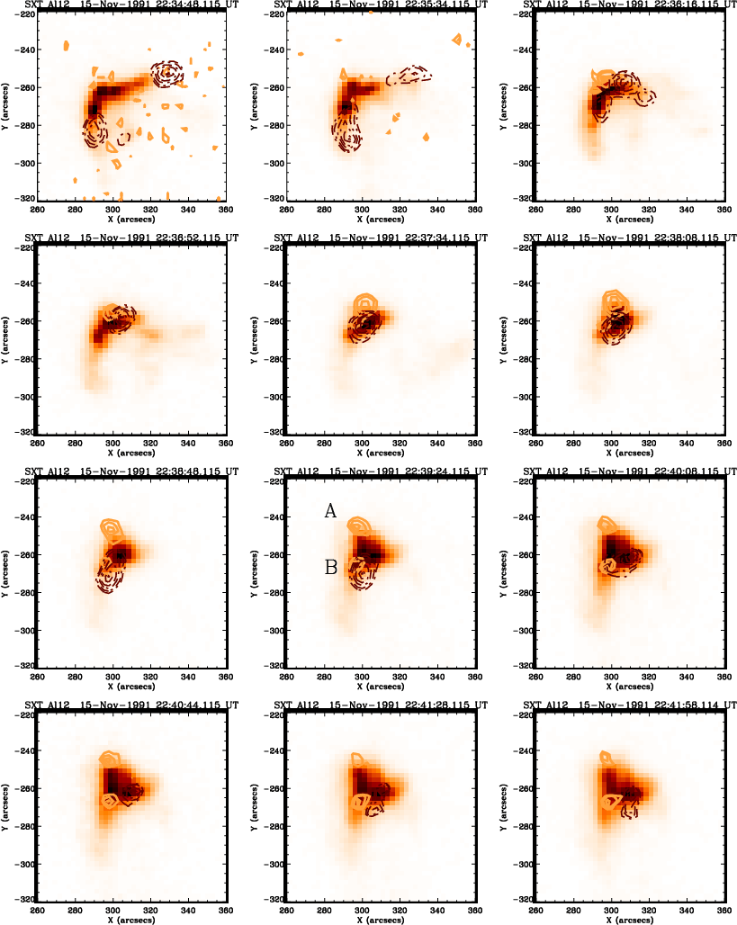$\begin{figure} \resizebox{16cm}{!}{\includegraphics{4109on.f22.ps}}\end{figure}$ Figure F.4: A series of images of the flare of 15 November 1991 in the Al12 filter of the SXT. Overlaid are contours of the WL emission (solid lines) and of the M1 channel (dashed lines).

In the text

$\begin{figure}\par\includegraphics{4109on.f23.ps}\end{figure}$ Figure G.1: Time series plots of the 17 November 1991 flare. Top panel: M2 cts/s/SC. Middle panel: WLF contrast calculated relative to the pre-flare brightness in the location that the flare occurred. Lower panel: GOES 1-8 Å flux. The vertical line indicates the time of maximum WLF contrast.

In the text

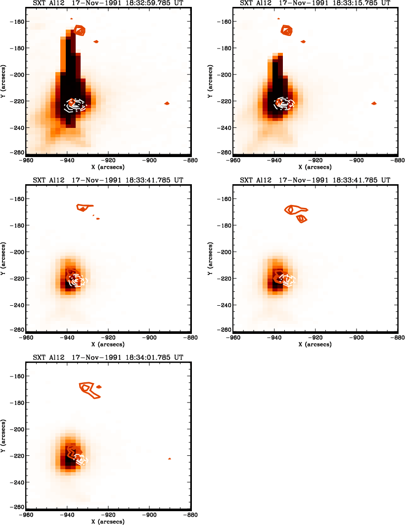$\begin{figure}\par\resizebox{16cm}{!}{\includegraphics{4109on.f24.ps}}\end{figure}$ Figure G.2: A series of images of the flare of 17 November 1991 in the Al12 filter of the SXT. Overlaid are contours of the WL emission (solid lines) and of the M1 channel (dashed lines).

In the text

$\begin{figure}\par\includegraphics{4109on.f25.ps}\end{figure}$ Figure H.1: Time series plots of the 3 December 1991 flare. Top panel: M2 cts/s/SC. Middle panel: WLF contrast calculated relative to the pre-flare brightness in the location that the flare occurred. Lower panel: GOES 1-8 Å flux. The vertical line indicates the time of maximum WLF contrast.

In the text

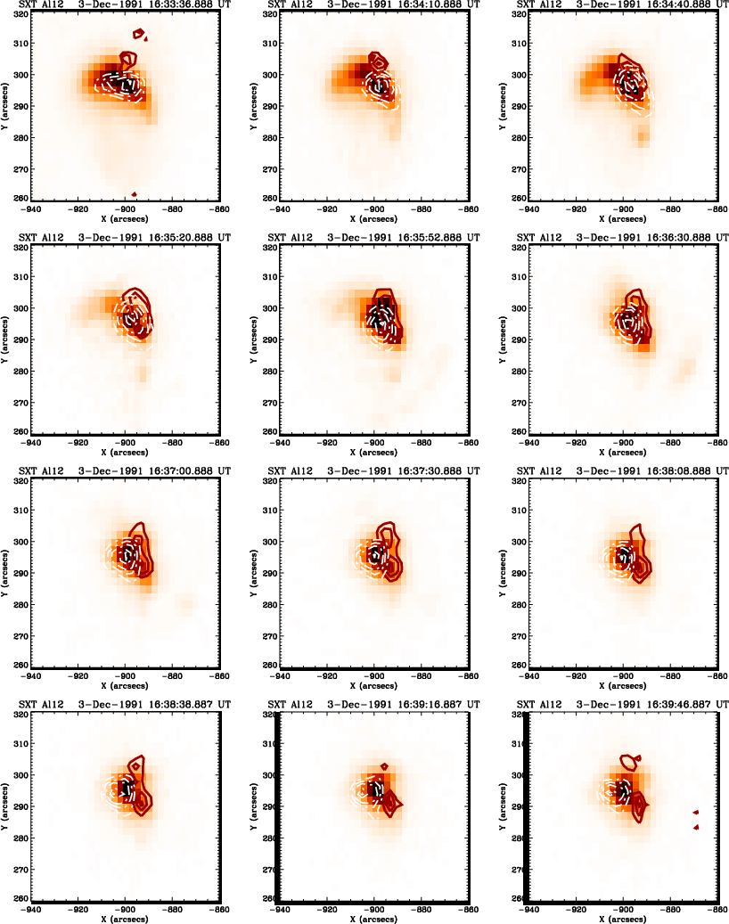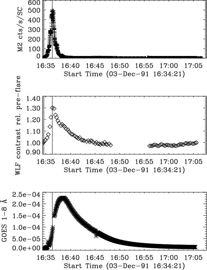
$\begin{figure}\par\resizebox{16cm}{!}{\includegraphics{4109on.f26.ps}}\end{figure}$ Figure H.2: A series of images of the flare of 3 December 1991 in the Al12 filter of the SXT. Overlaid are contours of the WL emission (solid lines) and of the M1 channel (dashed lines).

In the text

$\begin{figure}\includegraphics{4109on.f27.ps}\end{figure}$ Figure I.1: Time series plots of the 11 December 1991 flare. Top panel: M2 cts/s/SC. Middle panel: WLF contrast calculated relative to the pre-flare brightness in the location that the flare occurred. Lower panel: GOES 1-8 Å flux. The vertical line indicates the time of maximum WLF contrast.

In the text

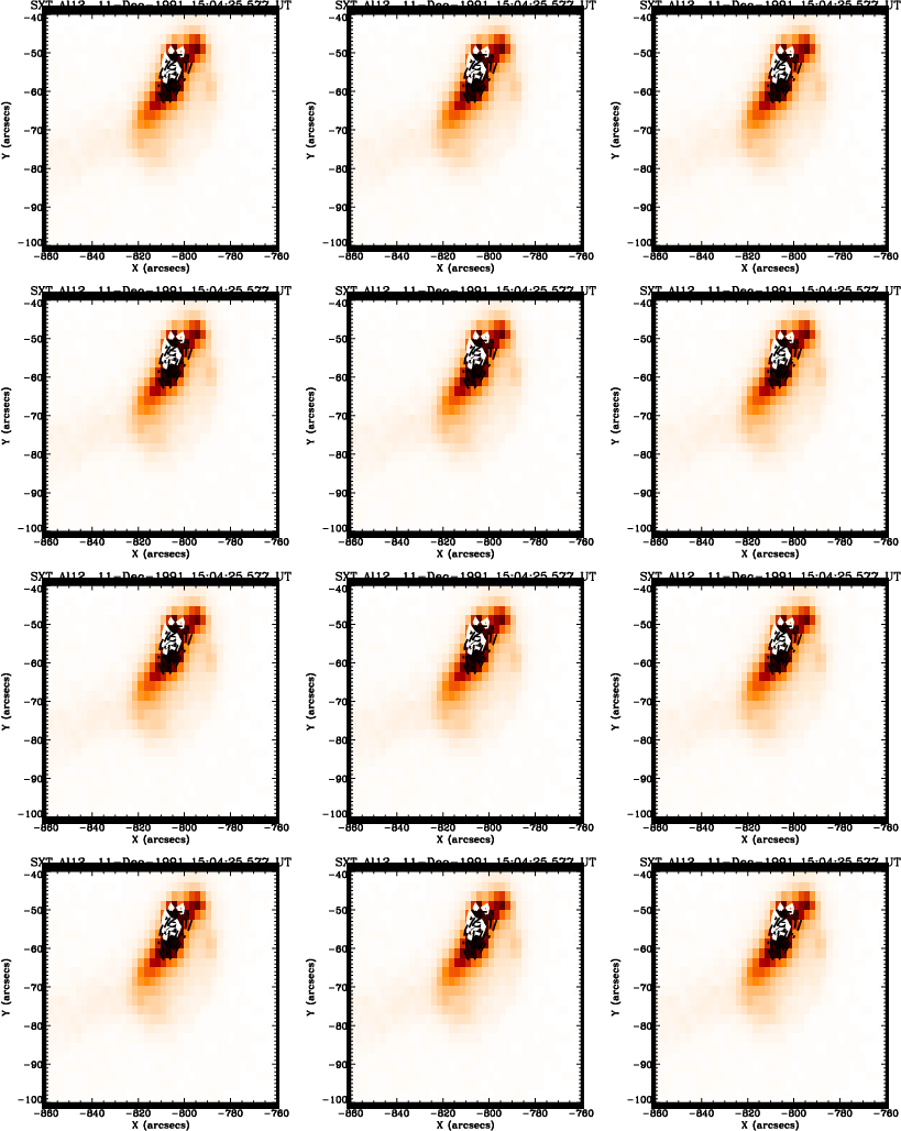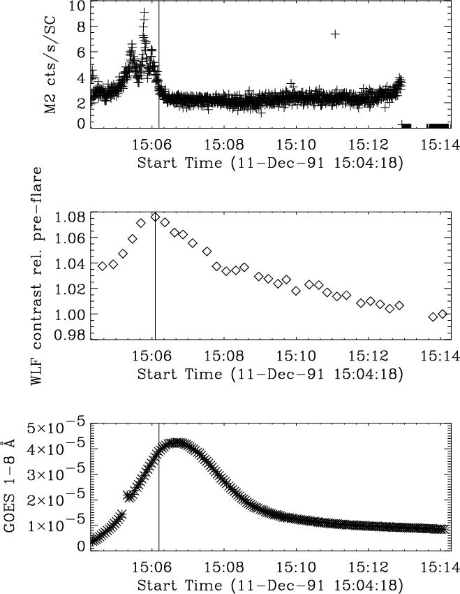
$\begin{figure}\par\resizebox{16cm}{!}{\includegraphics{4109on.f28.ps}}\end{figure}$ Figure I.2: A series of images of the flare of 11 December 1991 in the Al12 filter of the SXT. Overlaid are contours of the WL emission (solid lines) and of the M1 channel (dashed lines).

In the text

$\begin{figure}\par\includegraphics{4109on.f29.ps}\end{figure}$ Figure J.1: Time series plots of the 1st 16 December 1991 flare. Top panel: M2 cts/s/SC. Middle panel: WLF contrast calculated relative to the pre-flare brightness in the location that the flare occurred. Lower panel: GOES 1-8 Å flux. The vertical line indicates the time of maximum WLF contrast.

In the text

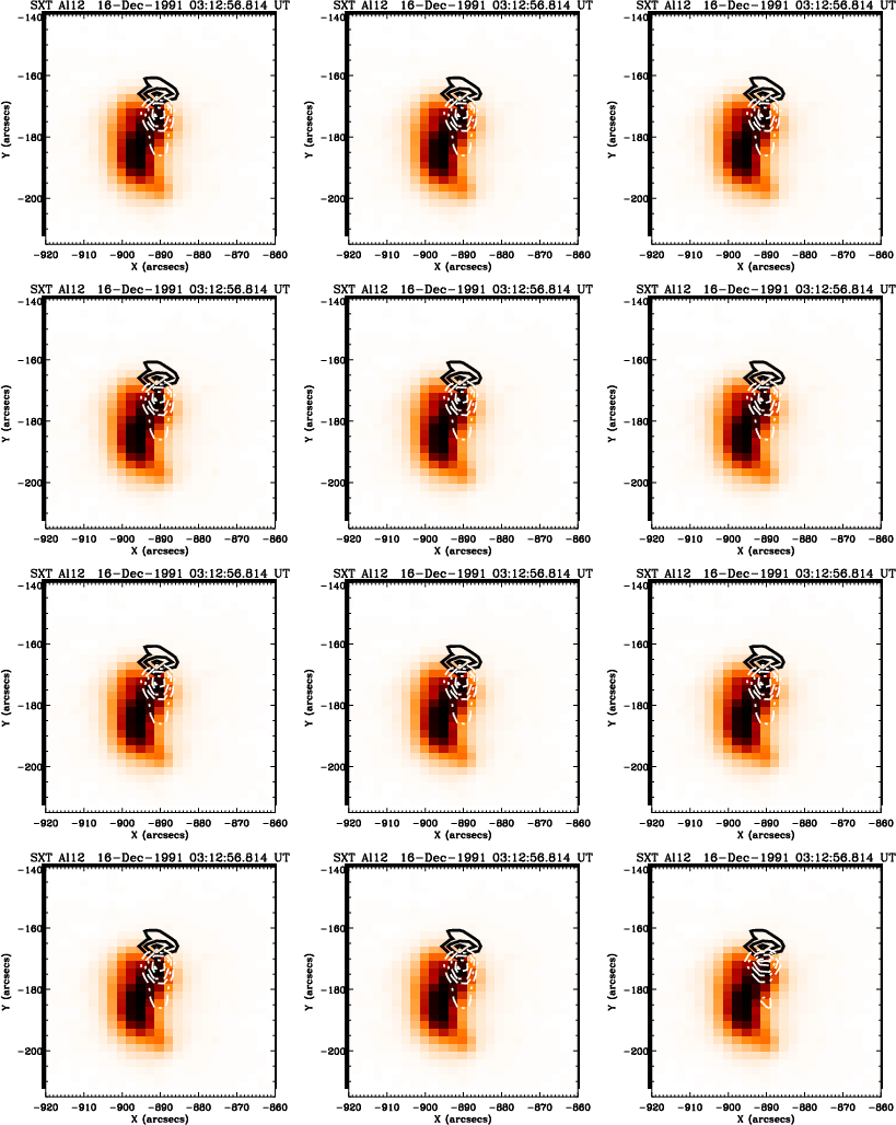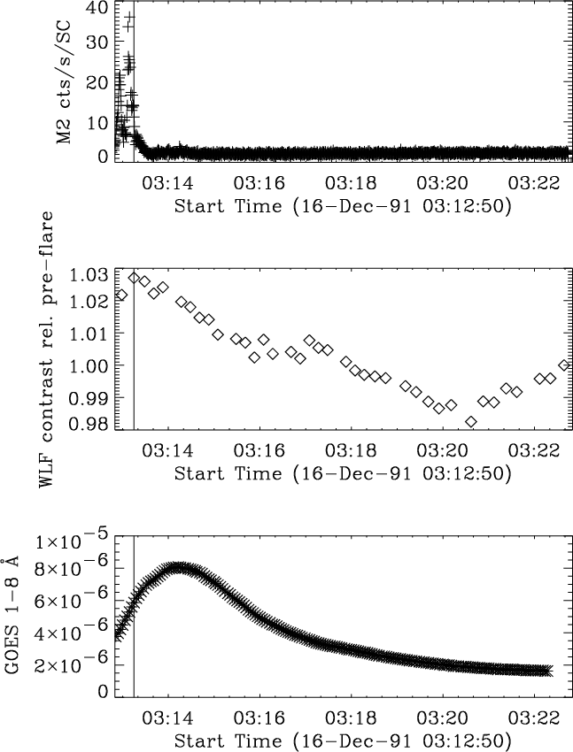
$\begin{figure}\par\resizebox{16cm}{!}{\includegraphics{4109on.f30.ps}}\end{figure}$ Figure J.2: A series of images of the 1st flare on 16 December 1991 in the Al12 filter of the SXT. Overlaid are contours of the WL emission (solid lines) and of the M1 channel (dashed lines).

In the text

$\begin{figure}\par\includegraphics{4109on.f31.ps}\end{figure}$ Figure K.1: Time series plots of the 16 December 1991 flare. Top panel: M2 cts/s/SC. Middle panel: WLF contrast calculated relative to the pre-flare brightness in the location that the flare occurred. Lower panel: GOES 1-8 Å flux. The vertical line indicates the time of maximum WLF contrast.

In the text

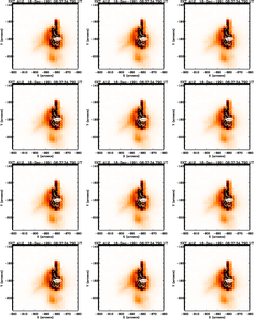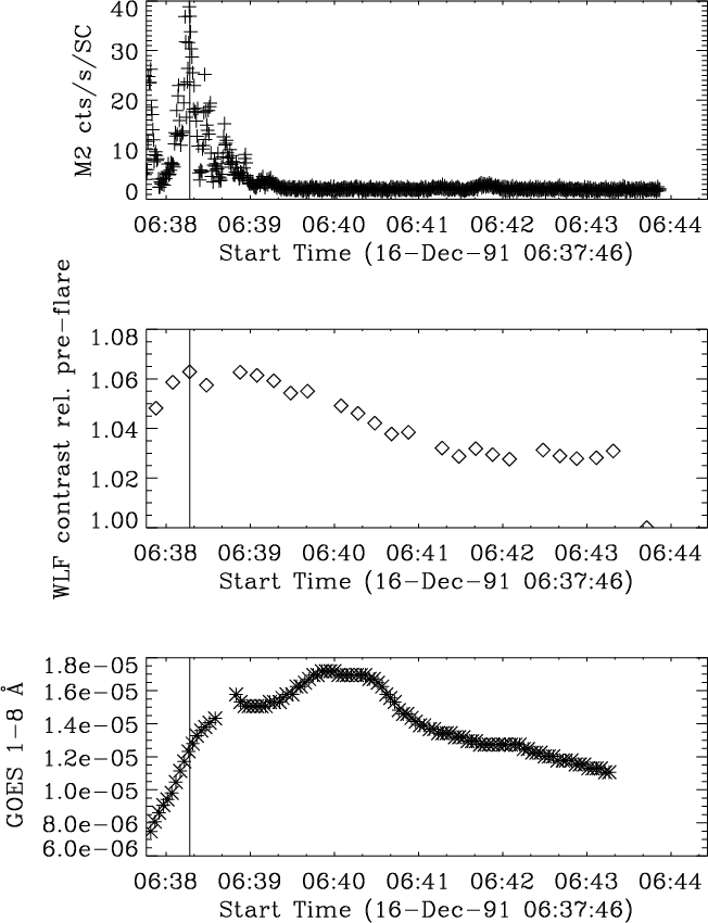
$\begin{figure}\par\resizebox{16cm}{!}{\includegraphics{4109on.f32.ps}}\end{figure}$ Figure K.2: A series of images of the flare of 16 December 1991 in the Al12 filter of the SXT. Overlaid are contours of the WL emission (solid lines) and of the M1 channel (dashed lines).

In the text

$\begin{figure}\par\includegraphics[width=8cm]{4109on.f33.ps}\end{figure}$ Figure L.1: Time series plots of the 26 December 1991 flare. Top panel: M2 cts/s/SC. Middle panel: WLF contrast calculated relative to the pre-flare brightness in the location that the flare occurred. Lower panel: GOES 1-8 Å flux. The vertical line indicates the time of maximum WLF contrast.

In the text

$\begin{figure}\includegraphics[width=8cm]{4109on.f34.ps}\end{figure}$ Figure L.2: Light-curves of the WLF, M2 and Al12 emission in kernel A of the flare of 26 December 1991 centred on (-330, -190). The Al12 and M2 curves have been scaled and shifted relative to the WLF curve for clarity. In this instance WLF cts are from the difference cube (DN/s). The vertical line marks the time of peak WLF cts in this kernel.

In the text

$\begin{figure}\includegraphics[width=8cm]{4109on.f35.ps}\end{figure}$ Figure L.3: Light-curves of the WLF, M2 and Al12 emission in kernel B of the flare of 26 December 1991 centred on (-310, -190). The Al12 and M2 curves have been scaled and shifted relative to the WLF curve for clarity. In this instance WLF cts are from the difference cube (DN/s). The vertical line marks the time of peak WLF cts in this kernel.

In the text

$\begin{figure}\par\includegraphics[width=8cm]{4109on.f36.ps}\end{figure}$ Figure L.4: Light-curves of the WLF, M2 and Al12 emission in kernel C of the flare of 26 December 1991 centred on (-260, -240). The Al12 and M2 curves have been scaled and shifted relative to the WLF curve for clarity. In this instance WLF cts are from the difference cube (DN/s). The vertical line marks the time of peak WLF cts in this kernel.

In the text

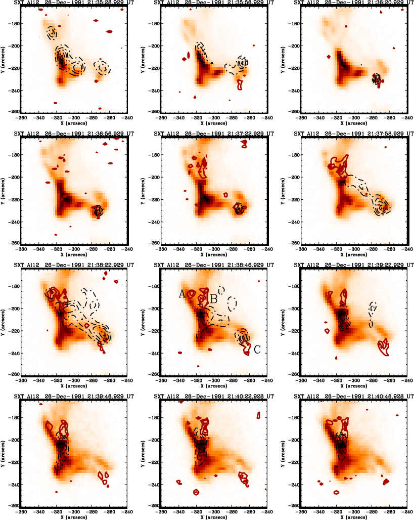$\begin{figure}\par\resizebox{16cm}{!}{\includegraphics{4109on.f37.ps}}\end{figure}$ Figure L.5: A series of images of the flare of 26 December 1991 in the Al12 filter of the SXT. Overlaid are contours of the WL emission (solid lines) and of the M1 channel (dashed lines).

In the text

$\begin{figure}\par\includegraphics{4109on.f38.ps}\def \@captype{figure}\end{figure}$ Figure M.1: Time series plots of the 28 December 1991 flare. Top panel: M2 cts/s/SC. Middle panel: WLF contrast calculated relative to the pre-flare brightness in the location that the flare occurred. Lower panel: GOES 1-8 Å flux. The vertical line indicates the time of maximum WLF contrast.

In the text

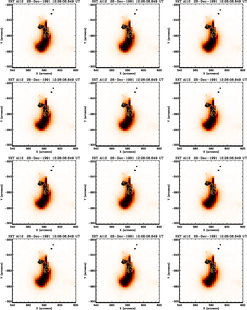$\begin{figure}\par\resizebox{16cm}{!}{\includegraphics{4109on.f39.ps}}\end{figure}$ Figure M.2: A series of images of the flare of 28 December 1991 in the Al12 filter of the SXT. Overlaid are contours of the WL emission (solid lines) and of the M1 channel (dashed lines).

In the text

$\begin{figure}\par\includegraphics[width=8cm]{4109on.f40.ps}\end{figure}$ Figure N.1: Time series plots of the 26 January 1992 flare. Top panel: M2 cts/s/SC. Middle panel: WLF contrast calculated relative to the pre-flare brightness in the location that the flare occurred. Lower panel: GOES 1-8 Å flux. The vertical line indicates the time of maximum WLF contrast.

In the text

$\begin{figure}\par\includegraphics[width=8cm]{4109on.f41.ps}\end{figure}$ Figure N.2: Light-curves of the WLF, M2 and Al12 emission in kernel A of the flare of 26 January 1992 centred on (875, -170). The Al12 and M2 curves have been scaled and shifted relative to the WLF curve for clarity. In this instance WLF cts are from the difference cube (DN/s). The vertical line marks the time of peak WLF cts in this kernel.

In the text

$\begin{figure}\includegraphics[width=8.5cm]{4109on.f42.ps}\end{figure}$ Figure N.3: Light-curves of the WLF, M2 and Al12 emission in kernel B of the flare of 26 January 1992 centred on (855, -215). The Al12 and M2 curves have been scaled and shifted relative to the WLF curve for clarity. In this instance WLF cts are from the difference cube (DN/s). The vertical line marks the time of peak WLF cts in this kernel.

In the text

$\begin{figure}\includegraphics[width=8.5cm]{4109on.f43.ps}\end{figure}$ Figure N.4: Light-curves of the WLF, M2 and Al12 emission in kernel C of the flare of 26 January 1992 centred on (865, -230). The Al12 and M2 curves have been scaled and shifted relative to the WLF curve for clarity. In this instance WLF cts are from the difference cube (DN/s). The vertical line marks the time of peak WLF cts in this kernel.

In the text

$\begin{figure}\includegraphics[width=8cm]{4109on.f44.ps}\def \@captype{figure}\end{figure}$ Figure N.5: Light-curves of the WLF, M2 and Al12 emission in kernel D of the flare of 26 January 1992 centred on (830, -220). The Al12 and M2 curves have been scaled and shifted relative to the WLF curve for clarity. In this instance WLF cts are from the difference cube (DN/s). The vertical line marks the time of peak WLF cts in this kernel.

In the text

$\begin{figure}\includegraphics[width=8cm]{4109on.f45.ps}\def \@captype{figure}\end{figure}$ Figure N.6: Light-curves of the WLF, M2 and Al12 emission in kernel E of the flare of 26 January 1992 centred on (845, -245). The Al12 and M2 curves have been scaled and shifted relative to the WLF curve for clarity. In this instance WLF cts are from the difference cube (DN/s). The vertical line marks the time of peak WLF cts in this kernel.

In the text

$\begin{figure}\par\resizebox{16cm}{!}{\includegraphics[width=16cm]{4109on.f46.ps}}\end{figure}$ Figure N.7: A series of images of the flare of 26 January 1992 in the Al12 filter of the SXT. Overlaid are contours of the WL emission (solid lines) and of the M1 channel (dashed lines).

In the text

$\begin{figure}\par\includegraphics{4109on.f47.ps}\def \@captype{figure}\end{figure}$ Figure O.1: Time series plots of the 30 January 1992 flare. Top panel: M2 cts/s/SC. Middle panel: WLF contrast calculated relative to the pre-flare brightness in the location that the flare occurred. Lower panel: GOES 1-8 Å flux. The vertical line indicates the time of maximum WLF contrast.

In the text

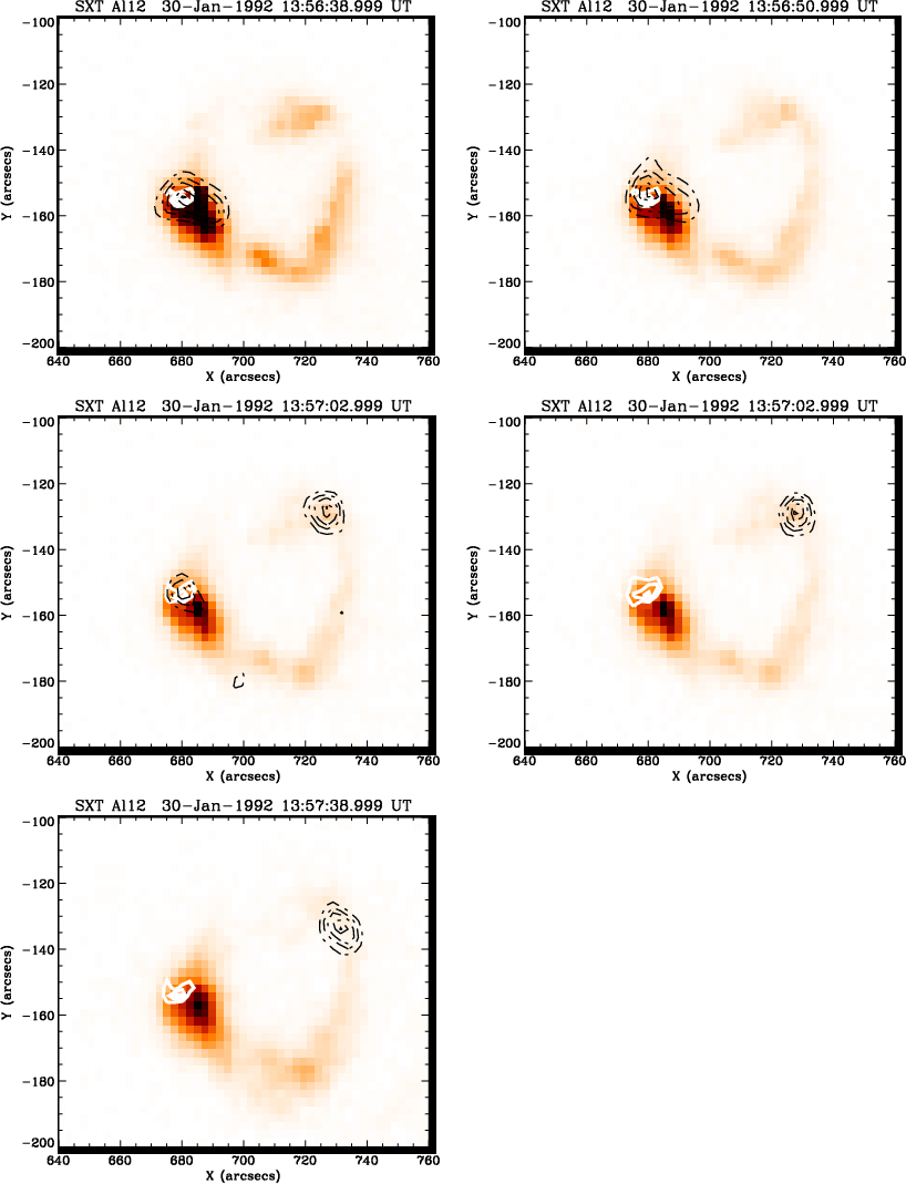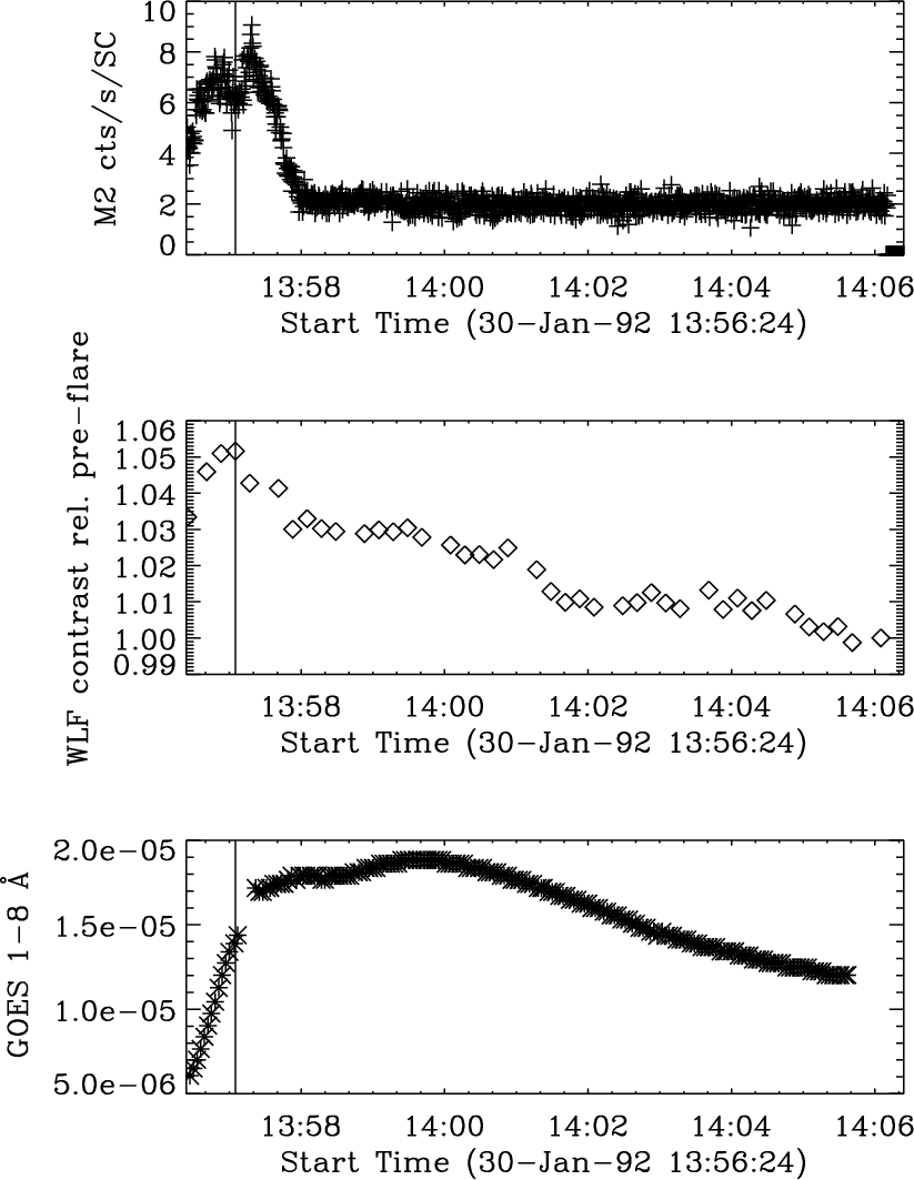
$\begin{figure}\par\resizebox{16cm}{!}{\includegraphics{4109on.f48.ps}}\end{figure}$ Figure O.2: A series of images of the flare of 30 January 1992 in the Al12 filter of the SXT. Overlaid are contours of the WL emission (solid lines) and of the M1 channel (dashed lines).

In the text

$\begin{figure}\par\includegraphics[width=8cm]{4109on.f49.ps}\end{figure}$ Figure P.1: Time series plots of the 6 February 1992 flare. Top panel: M2 cts/s/SC. Middle panel: WLF contrast calculated relative to the pre-flare brightness in the location that the flare occurred. Lower panel: GOES 1-8 Å flux. The vertical line indicates the time of maximum WLF contrast.

In the text

$\begin{figure}\includegraphics[width=8cm]{4109on.f50.ps}\end{figure}$ Figure P.2: Light-curves of the WLF, M2 and Al12 emission in kernel A of the flare of 6 February 1992 centred on (960,145). The Al12 and M2 curves have been scaled and shifted relative to the WLF curve for clarity. In this instance WLF cts are from the difference cube (DN/s). The vertical line marks the time of peak WLF cts in this kernel.

In the text

$\begin{figure}\includegraphics[width=8cm]{4109on.f51.ps}\end{figure}$ Figure P.3: Light-curves of the WLF, M2 and Al12 emission in kernel B of the flare of 6 February 1992 centred on (960,125). The Al12 and M2 curves have been scaled and shifted relative to the WLF curve for clarity. In this instance WLF cts are from the difference cube (DN/s). The vertical line marks the time of peak WLF cts in this kernel.

In the text

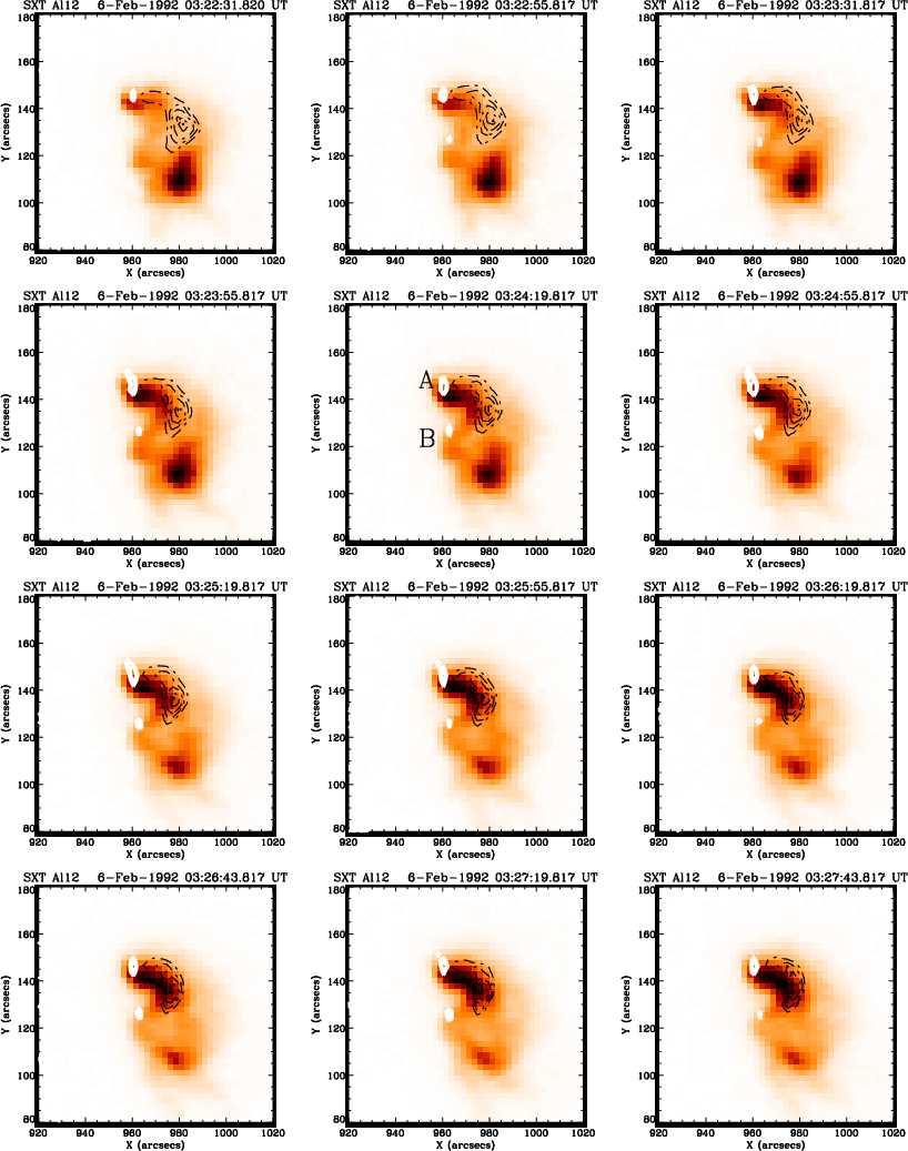$\begin{figure}\par\resizebox{16cm}{!}{\includegraphics{4109on.f52.ps}}\end{figure}$ Figure P.4: A series of images of the flare of 6 February 1992 in the Al12 filter of the SXT. Overlaid are contours of the WL emission (solid lines) and of the M1 channel (dashed lines).

In the text

$\begin{figure}\par\includegraphics[width=8cm]{4109on.f53.ps}\end{figure}$ Figure Q.1: Time series plots of the 15 February 1992 flare. Top panel: M2 cts/s/SC. Middle panel: WLF contrast calculated relative to the pre-flare brightness in the location that the flare occurred. Lower panel: GOES 1-8 Å flux. The vertical line indicates the time of maximum WLF contrast.

In the text

$\begin{figure}\includegraphics[width=8cm]{4109on.f54.ps}\end{figure}$ Figure Q.2: Light-curves of the WLF, M2 and Al12 emission in kernel A of the flare of 15 February 1992 centred on (230, -120). The Al12 and M2 curves have been scaled and shifted relative to the WLF curve for clarity. In this instance WLF cts are from the difference cube (DN/s). The vertical line marks the time of peak WLF cts in this kernel.

In the text

$\begin{figure}\includegraphics[width=8cm]{4109on.f55.ps}\end{figure}$ Figure Q.3: Light-curves of the WLF, M2 and Al12 emission in kernel B of the flare of 15 February 1992 centred on (190, -130). The Al12 and M2 curves have been scaled and shifted relative to the WLF curve for clarity. In this instance WLF cts are from the difference cube (DN/s). The vertical line marks the time of peak WLF cts in this kernel.

In the text

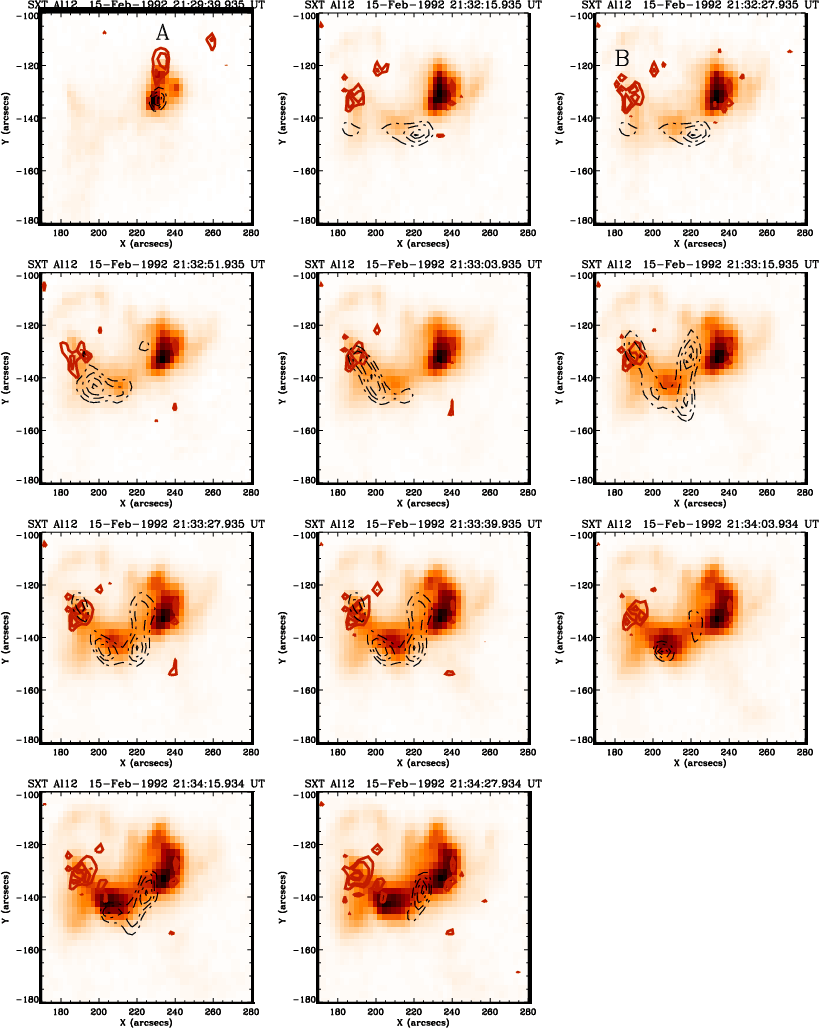$\begin{figure}\par\resizebox{16cm}{!}{\includegraphics{4109on.f56.ps}}\end{figure}$ Figure Q.4: A series of images of the flare of 15 February 1992 in the Al12 filter of the SXT. Overlaid are contours of the WL emission (solid lines) and of the M1 channel (dashed lines).

In the text

$\begin{figure}\par\includegraphics{4109on.f57.ps}\end{figure}$ Figure R.1: Time series plots of the 24 April 1992 flare. Top panel: M2 cts/s/SC. Middle panel: WLF contrast calculated relative to the pre-flare brightness in the location that the flare occurred. Lower panel: GOES 1-8 Å flux. The vertical line indicates the time of maximum WLF contrast.

In the text

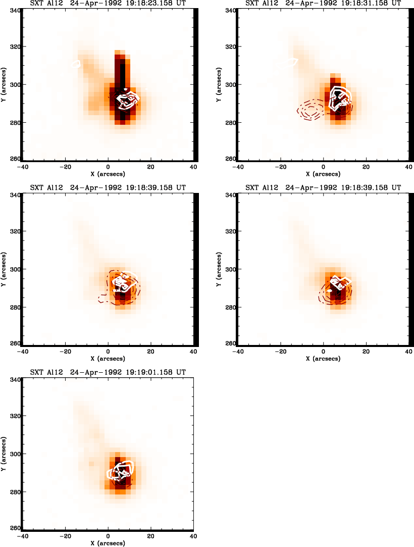$\begin{figure}\par\resizebox{16cm}{!}{\includegraphics{4109on.f58.ps}}\end{figure}$ Figure R.2: A series of images of the flare of 24 April 1992 in the Al12 filter of the SXT. Overlaid are contours of the WL emission (solid lines) and of the M1 channel (dashed lines).

In the text

$\begin{figure}\par\includegraphics[width=8cm]{4109on.f59.ps}\end{figure}$ Figure S.1: Time series plots of the 16 July 1992 flare. Top panel: M2 cts/s/SC. Middle panel: WLF contrast calculated relative to the pre-flare brightness in the location that the flare occurred. Lower panel: GOES 1-8 Å flux. The vertical line indicates the time of maximum WLF contrast.

In the text

$\begin{figure}\includegraphics[width=8cm]{4109on.f60.ps}\end{figure}$ Figure S.2: Light-curves of the WLF, M2 and Al12 emission in kernel A of the flare of 16 July 1992 centred on (810, -195). The Al12 and M2 curves have been scaled and shifted relative to the WLF curve for clarity. In this instance WLF cts are from the difference cube (DN/s). The vertical line marks the time of peak WLF cts in this kernel.

In the text

$\begin{figure}\includegraphics[width=8cm]{4109on.f61.ps}\end{figure}$ Figure S.3: Light-curves of the WLF, M2 and Al12 emission in kernel B of the flare of 16 July 1992 centred on (810, -175). The Al12 and M2 curves have been scaled and shifted relative to the WLF curve for clarity. In this instance WLF cts are from the difference cube (DN/s). The vertical line marks the time of peak WLF cts in this kernel.

In the text

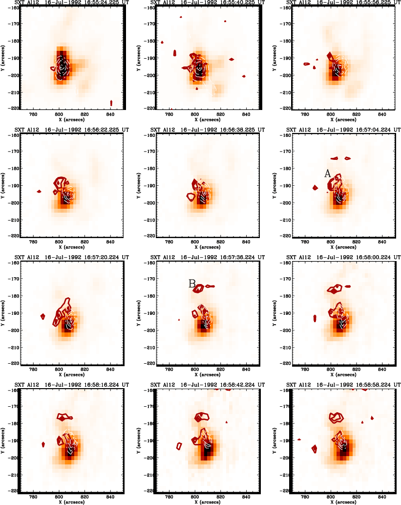$\begin{figure}\par\resizebox{16cm}{!}{\includegraphics{4109on.f62.ps}}\end{figure}$ Figure S.4: A series of images of the flare of 16 July 1992 in the Al12 filter of the SXT. Overlaid are contours of the WL emission (solid lines) and of the M1 channel (dashed lines).

In the text

$\begin{figure}\par\includegraphics{4109on.f63.ps}\end{figure}$ Figure T.1: Time series plots of the 11 August 1992 flare. Top panel: M2 cts/s/SC. Middle panel: WLF contrast calculated relative to the pre-flare brightness in the location that the flare occurred. Lower panel: GOES 1-8 Å flux. The vertical line indicates the time of maximum WLF contrast.

In the text

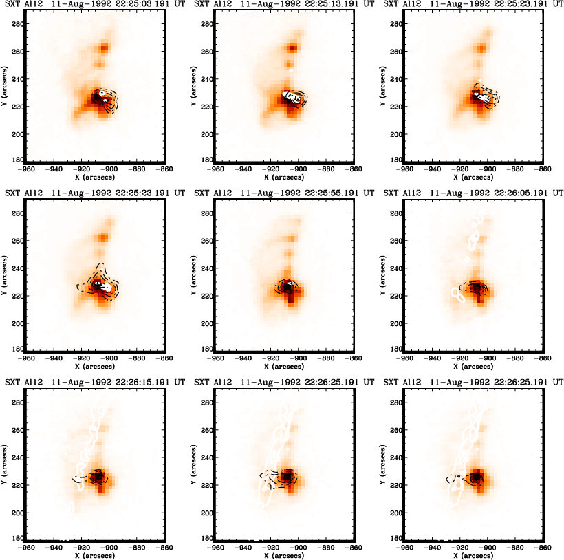$\begin{figure}\par\resizebox{16cm}{!}{\includegraphics{4109on.f64.ps}}\end{figure}$ Figure T.2: A series of images of the flare of 11 August 1992 in the Al12 filter of the SXT. Overlaid are contours of the WL emission (solid lines) and of the M1 channel (dashed lines).

In the text

$\begin{figure}\par\includegraphics{4109on.f65.ps}\end{figure}$ Figure U.1: Time series plots of the 20 August 1992 flare. Top panel: M2 cts/s/SC. Middle panel: WLF contrast calculated relative to the pre-flare brightness in the location that the flare occurred. Lower panel: GOES 1-8 Å flux. The vertical line indicates the time of maximum WLF contrast.

In the text

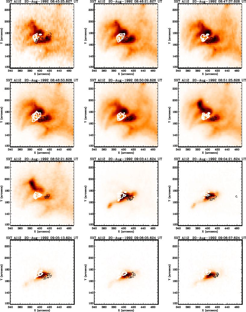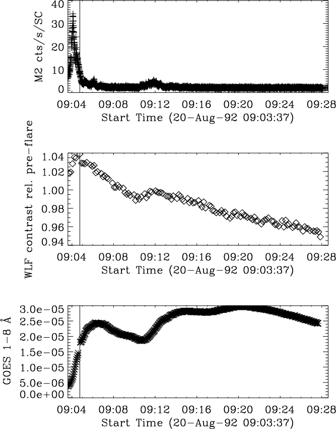
$\begin{figure}\par\resizebox{16cm}{!}{\includegraphics{4109on.f66.ps}}\end{figure}$ Figure U.2: A series of images of the flare of 20 August 1992 in the Al12 filter of the SXT. Overlaid are contours of the WL emission (solid lines) and of the M1 channel (dashed lines).

In the text

$\begin{figure}\par\includegraphics{4109on.f67.ps}\def \@captype{figure}\end{figure}$ Figure V.1: Time series plots of the 6 September 1992 flare. Top panel: M2 cts/s/SC. Middle panel: WLF contrast calculated relative to the pre-flare brightness in the location that the flare occurred. Lower panel: GOES 1-8 Å flux. The vertical line indicates the time of maximum WLF contrast.

In the text

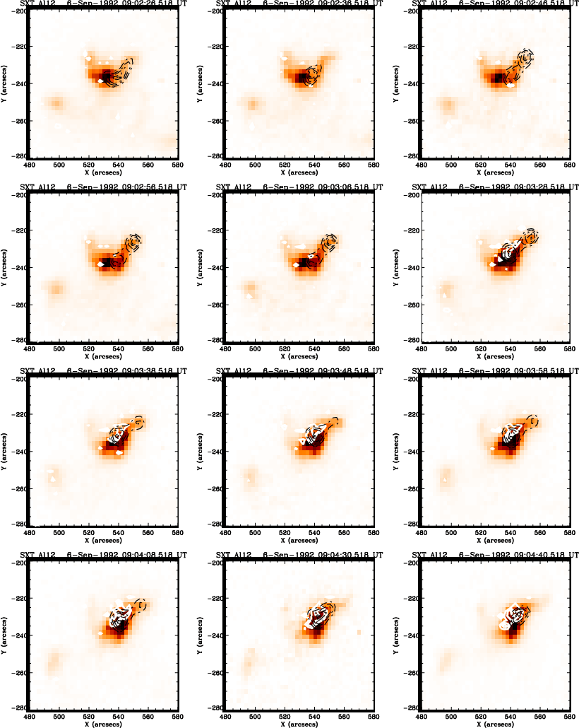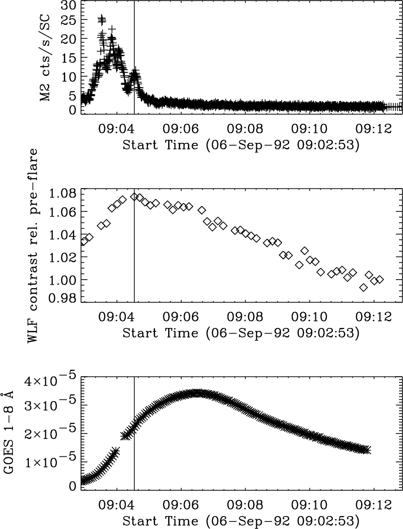
$\begin{figure}\par\resizebox{16cm}{!}{\includegraphics{4109on.f68.ps}}\end{figure}$ Figure V.2: A series of images of the flare of 6 September 1992 in the Al12 filter of the SXT. Overlaid are contours of the WL emission (solid lines) and of the M1 channel (dashed lines).

In the text

$\begin{figure}\par\includegraphics{4109on.f69.ps}\end{figure}$ Figure W.1: Time series plots of the 7 September 1992 flare. Top panel: M2 cts/s/SC. Middle panel: WLF contrast calculated relative to the pre-flare brightness in the location that the flare occurred. Lower panel: GOES 1-8 Å flux. The vertical line indicates the time of maximum WLF contrast.

In the text

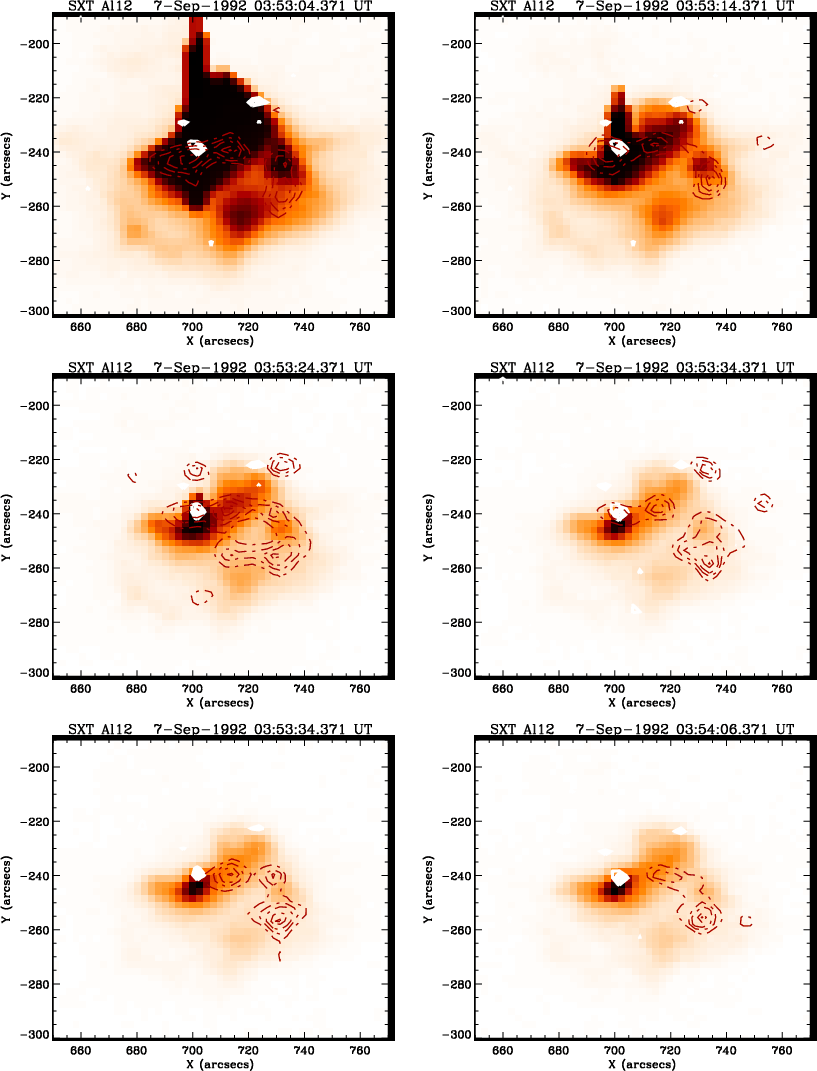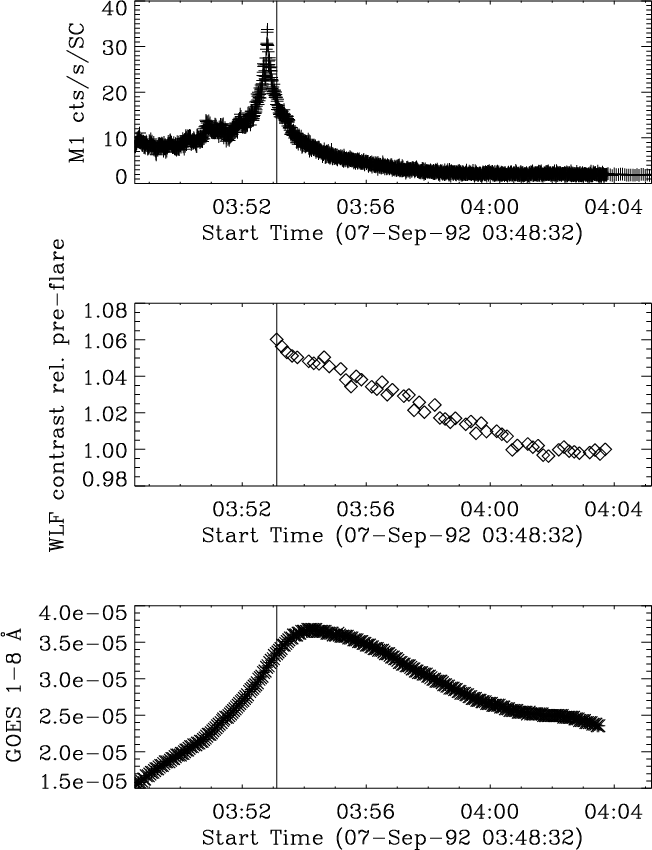
$\begin{figure}\par\resizebox{16cm}{!}{\includegraphics{4109on.f70.ps}}\end{figure}$ Figure W.2: A series of images of the flare of 7 September 1992 in the Al12 filter of the SXT. Overlaid are contours of the WL emission (solid lines) and of the M1 channel (dashed lines).

In the text

$\begin{figure}\par\includegraphics[width=8cm]{4109on.f71.ps}\end{figure}$ Figure X.1: Time series plots of the 10 September 1992 flare. Top panel: M2 cts/s/SC. Middle panel: WLF contrast calculated relative to the pre-flare brightness in the location that the flare occurred. Lower panel: GOES 1-8 Å flux. The vertical line indicates the time of maximum WLF contrast.

In the text

$\begin{figure}\includegraphics[width=8cm]{4109on.f72.ps}\end{figure}$ Figure X.2: Light-curves of the WLF, M2 and Al12 emission in kernel A of the flare of 10 September 1992 centred on (-620,225). The Al12 and M2 curves have been scaled and shifted relative to the WLF curve for clarity. In this instance WLF cts are from the difference cube (DN/s). The vertical line marks the time of peak WLF cts in this kernel.

In the text

$\begin{figure}\includegraphics[width=8cm]{4109on.f73.ps}\end{figure}$ Figure X.3: Light-curves of the WLF, M2 and Al12 emission in kernel B of the flare of 10 September 1992 centred on (-620,195). The Al12 and M2 curves have been scaled and shifted relative to the WLF curve for clarity. In this instance WLF cts are from the difference cube (DN/s). The vertical line marks the time of peak WLF cts in this kernel.

In the text

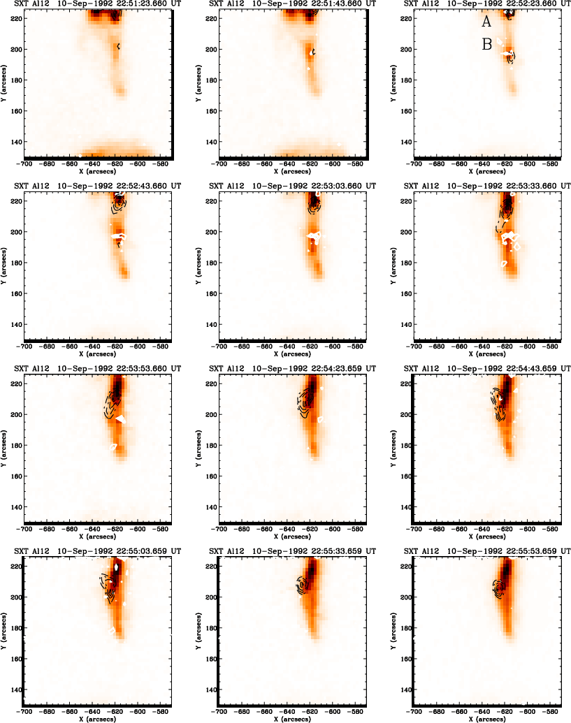$\begin{figure}\par\resizebox{16cm}{!}{\includegraphics{4109on.f74.ps}}\end{figure}$ Figure X.4: A series of images of the flare of 10 September 1992 in the Al12 filter of the SXT. Overlaid are contours of the WL emission (solid lines) and of the M1 channel (dashed lines).

In the text

$\begin{figure}\par\includegraphics{4109on.f75.ps}\end{figure}$ Figure Y.1: Time series plots of the 5 November 1992 flare. Top panel: M2 cts/s/SC. Middle panel: WLF contrast calculated relative to the pre-flare brightness in the location that the flare occurred. Lower panel: GOES 1-8 Å flux. The vertical line indicates the time of maximum WLF contrast.

In the text

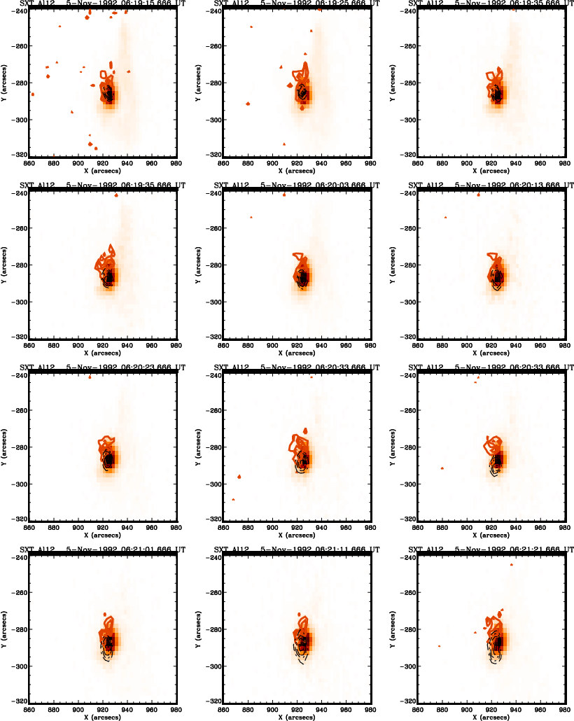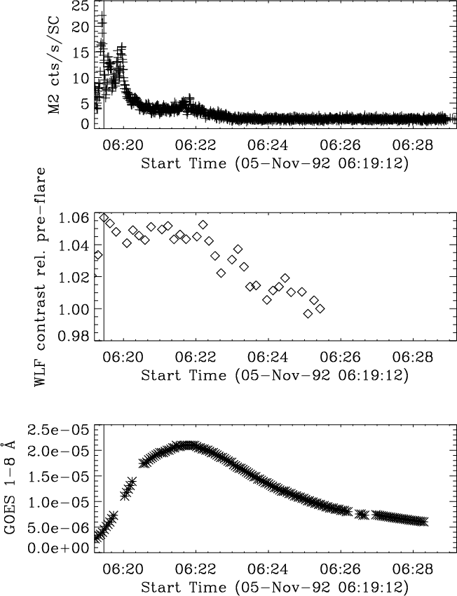
$\begin{figure}\par\resizebox{16cm}{!}{\includegraphics{4109on.f76.ps}}\end{figure}$ Figure Y.2: A series of images of the flare of 5 November 1992 in the Al12 filter of the SXT. Overlaid are contours of the WL emission (solid lines) and of the M1 channel (dashed lines).

In the text

$\begin{figure} \par\resizebox{\hsize}{!}{\includegraphics{4109.f2.ps}}\end{figure}$	Figure 2: Time series plots of the 2 November 1991 flare. Top panel: M2 cts/s/SC. Middle panel: WLF contrast calculated relative to the pre-flare brightness in the location that the flare occurred. Lower panel: GOES 1-8 Å flux. The vertical line indicates the time of maximum WLF contrast.
Open with DEXTER

$\begin{figure} \par\resizebox{8.5cm}{!}{\includegraphics{4109.f3.ps}}\end{figure}$	Figure 3: Light-curves of the WLF, M2 and Al12 emission in the northern most kernel A of the flare of 2 November 1991, centred on (820, -235). The Al12 and M2 curves have been scaled and shifted relative to the WLF curve for clarity. In this instance WLF cts are from the difference cube (DN/s). The vertical line marks the time of peak WLF cts in this kernel.
Open with DEXTER

$\begin{figure} \par\resizebox{8.5cm}{!}{\includegraphics{4109.f4.ps}}\end{figure}$	Figure 4: Light-curves of the WLF, M2 and Al12 emission in kernel B of the flare of 2 November 1991 centred on (850, -260). The Al12 and M2 curves have been scaled and shifted relative to the WLF curve for clarity. In this instance WLF cts are from the difference cube (DN/s). The vertical line marks the time of peak WLF cts in this kernel.
Open with DEXTER

$\begin{figure} \par\resizebox{8.4cm}{!}{\includegraphics{4109.f6.ps}}\end{figure}$	Figure 6: Time series plots of the 8 July 1992 flare. Top panel: M2 cts/s/SC. Middle panel: WLF contrast calculated relative to the pre-flare brightness in the location that the flare occurred. Lower panel: GOES 1-8 Å flux. The vertical line indicates the time of maximum WLF contrast.
Open with DEXTER

$\begin{figure} \par\resizebox{8.2cm}{!}{\includegraphics{4109.f7.ps}}\end{figure}$	Figure 7: Light-curves of the WLF, M2 and Al12 emission in source A for the 8 July 1992 flare centred at (-665, -235). The Al12 and M2 curves have been scaled and shifted relative to the WLF curve for clarity. In this instance WLF cts are from the difference cube (DN/s).
Open with DEXTER

$\begin{figure} \par\resizebox{8.3cm}{!}{\includegraphics{4109.f8.ps}}\end{figure}$	Figure 8: Light-curves of the WLF, M2 and Al12 emission in source B for the 8 July 1992 flare centred at (-620, -240). The Al12 and M2 curves have been scaled and shifted relative to the WLF curve for clarity. In this instance WLF cts are from the difference cube (DN/s).
Open with DEXTER

$\begin{figure} \par\resizebox{15.9cm}{!}{\includegraphics{4109.f9.ps}}\end{figure}$	Figure 9: A series of images of the flare of 14 February 1992 in the Al12 filter of the SXT. Overlaid are contours of the WL emission (solid lines) and of the M1 channel (dashed black line). There are 5 WLF kernels, 4 of which correlate well spatially with the M1 sources during the impulsive phase of the flare.
Open with DEXTER

$\begin{figure} \par\resizebox{8.5cm}{!}{\includegraphics{4109.f10.ps}}\end{figure}$	Figure 10: Time series plots of the 14 February 1992 flare. Top panel: M2 cts/s/SC. Middle panel: WLF contrast calculated relative to the pre-flare brightness in the location that the flare occurred. Lower panel: GOES 1-8 Å flux. The vertical line indicates the time of maximum WLF contrast.
Open with DEXTER

$\begin{figure} \par\resizebox{8.3cm}{!}{\includegraphics{4109.f11.ps}}\end{figure}$	Figure 11: Light-curves of the WLF, M2 and Al12 emission in the northern most kernel (A) of the flare of 14 February 1992, centred on (-60, -70). The Al12 and M2 curves have been scaled and shifted relative to the WLF curve for clarity. In this instance WLF cts are from the difference cube (DN/s).
Open with DEXTER

$\begin{figure} \par\resizebox{8.5cm}{!}{\includegraphics{4109.f12.ps}}\end{figure}$	Figure 12: Light-curves of the WLF, M2 and Al12 emission in kernel B of the flare of 14 February 1992, centred on (-50, -85). The Al12 and M2 curves have been scaled and shifted relative to the WLF curve for clarity. In this instance WLF cts are from the difference cube (DN/s).
Open with DEXTER

$\begin{figure} \par\resizebox{8.7cm}{!}{\includegraphics{4109.f13.ps}}\end{figure}$	Figure 13: Light-curves of the WLF, M2 and Al12 emission in kernel C of the flare of 14 February 1992, centred on (-55, -95). The Al12 and M2 curves have been scaled and shifted relative to the WLF curve for clarity. In this instance WLF cts are from the difference cube (DN/s).
Open with DEXTER

$\begin{figure} \par\resizebox{8.5cm}{!}{\includegraphics{4109.f14.ps}}\end{figure}$	Figure 14: Light-curves of the WLF, M2 and Al12 emission in kernel D of the flare of 14 February 1992, centred on (-20, -95). The Al12 and M2 curves have been scaled and shifted relative to the WLF curve for clarity. In this instance WLF cts are from the difference cube (DN/s).
Open with DEXTER

$\begin{figure} \par\resizebox{8.3cm}{!}{\includegraphics{4109.f15.ps}}\end{figure}$	Figure 15: Light-curves of the WLF, M2 and Al12 emission in the northern most kernel E of the flare of 14 February 1992, centred on (0, -95). The Al12 and M2 curves have been scaled and shifted relative to the WLF curve for clarity. In this instance WLF cts are from the difference cube (DN/s).
Open with DEXTER

$\begin{figure} \par\resizebox{15.5cm}{!}{\includegraphics{4109.f17.ps}}\end{figure}$	Figure 17: Histogram showing the distribution of electron beam power for non-WLFs, WLFs with peak contrast <5% and WLFs with peak contrast >5%.
Open with DEXTER

$\begin{figure} \par\resizebox{8.3cm}{!}{\includegraphics{4109.f18.ps}}\end{figure}$	Figure 18: Scatter plot showing the relationship between the peak electron beam power calculated for a thick target assumption and a low energy cut-off of 20 keV and the maximum WLF contrast relative to the pre-flare continuum intensity in the flare region.
Open with DEXTER

$\begin{figure} \par\resizebox{8cm}{!}{\includegraphics{4109.f19.ps}}\end{figure}$	Figure 19: Scatter plot showing the relationship between the peak GOES flux in the 1-8 Å channel and the peak value of M2/M1 for both non-WLFs and WLFs. * represents the non-WLFs and $\diamond$ represents the WLFs, with larger symbol size corresponding to those events that showed WLF contrast $\geq$ 5% relative to the pre-flare continuum intensity in the flare region.
Open with DEXTER

$\begin{figure} \par\resizebox{8cm}{!}{\includegraphics{4109.f20.ps}}\end{figure}$	Figure 20: Scatter plot showing the relationship between the peak value of M2/M1 and the peak WLF contrast relative to the pre-flare continuum intensity in the flare region. Here * represents the non-WLFs and $\diamond$ represents the WLFs.
Open with DEXTER

$\begin{figure} \par\resizebox{8cm}{!}{\includegraphics{4109.f22.ps}}\end{figure}$	Figure 22: Scatter plot showing peak coronal pressure against peak Be 119 flux. * represents non-WLFs, and $\diamond$ represents WLFs.
Open with DEXTER

$\begin{figure} \par\resizebox{8.4cm}{!}{\includegraphics{4109.f23.ps}}\end{figure}$	Figure 23: Scatter plot showing peak coronal pressure against peak GOES intensity. * represents non-WLFs, and $\diamond$ represents WLFs, with larger symbols representing higher contrast. Note that the flare with largest GOES flux was the 27 October 91 event, which was poorly observed preventing us from accurately deriving the contrast.
Open with DEXTER

$\begin{figure} \par\resizebox{8.2cm}{!}{\includegraphics{4109.f24.ps}}\end{figure}$	Figure 24: Scatter plot showing SXR scale length = $\sqrt {area > FWHM}$ against peak GOES intensity. Here * represents non-WLFs, and $\diamond$ represents WLFs. Note that the flare with largest GOES flux was the27 October 91 event, which was poorly observed preventing us from accurately deriving the contrast.
Open with DEXTER