![[*]](/icons/foot_motif.gif)
A&A 409, 1-7 (2003)
DOI: 10.1051/0004-6361:20031080
Wei-Min Gu1,2 - T. Foglizzo1
1 - Service d'Astrophysique, CEA/DSM/DAPNIA, CEA-Saclay,
91191 Gif-sur-Yvette, France
2 -
Department of Physics, Xiamen University,
Xiamen, Fujian 361005, PR China
Received 10 April 2003 / Accepted 30 June 2003
Abstract
The linear stability of a shocked isothermal accretion flow
onto a black hole is investigated in the inviscid limit.
The outer shock solution, which was previously found to be stable with
respect to axisymmetric perturbations, is, however, generally unstable to
non-axisymmetric ones.
Eigenmodes and growth rates are obtained by numerical integration of
the linearized equations.
The mechanism of this instability is based on the cycle of acoustic
waves between their corotation radius and the shock.
It is a form of
the Papaloizou-Pringle instability, modified by
advection and the presence of the shock. As such it can be
generalized to non isothermal shocked accretion flows. Blobs and
vortices are generated by the shock as a by-product of the
instability.
Key words: accretion, accretion disks - black hole physics - hydrodynamics - instabilities - shock waves
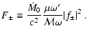
Hydrodynamic instabilities of shocked accretion flows may explain some of the properties of X-ray binaries, such as their time variability. The structure of stationary accretion flows involving shocks was described by Fukue (1987) and Chakarabarti (1989a,b). Even with the simple inviscid hypothesis, the structure of shocked accretion flows is complex, and their stability is not yet fully understood. As noted by Nakayama (1992), the calculations of Chakrabarti (1989a,b) are a study of the forced oscillations of the flow rather than an analysis of its intrinsic stability. Nakayama (1992, 1993) introduced a new type of global instability between the inner sonic point and the shock. He found that, of the two possible shock positions, the inner one is unstable due to post-shock acceleration, while the outer one is stable due to post-shock deceleration. His conclusion was confirmed by Nobuta & Hanawa (1994), whose numerical simulations showed that the inner shock is completely destroyed by perturbations, while the outer one is stable. All the above works, however, were based on axisymmetric calculations. Molteni et al. (1999, hereafter MTK) performed 2D simulations of an adiabatic flow with an outer shock and found a non-axisymmetric instability. They showed that the instability saturates at a low level, and a new asymmetric configuration develops, with a deformed shock rotating steadily. MTK pointed out that this effect may have relevant observational consequences, such as quasi-periodic oscillations (QPO). The mechanism of the instability was not explained by MTK, who briefly mentioned a possible link with the numerical simulations of Blaes & Hawley (1988). The Papaloizou-Pringle instability (1984, hereafter PPI) simulated by Blaes & Hawley is known to take place in discs or tori, in which the radial velocity is initially zero, whereas the flow simulated by MTK involves radial advection, an inner sonic point and an outer shock. The effect of advection on the PPI was investigated by Blaes (1987), who found that the PPI is strongly stabilized by advection at the inner boundary. The interpretation of the results of MTK in terms of the PPI is thus not obvious a priori. What is more, the flow studied by MTK is also potentially unstable by the advective-acoustic mechanism (Foglizzo & Tagger 2000; Foglizzo 2001, 2002), based on the cycle of entropy/vorticity perturbations and acoustic waves in the subsonic region between a stationary shock and a sonic surface.
The aim of this study is thus to understand the instability mechanism at work in shocked accretion flows. For the sake of simplicity, the present linear stability analysis is focused on isothermal accretion flows with constant angular momentum. The paper is organised as follows. Linearized equations and boundary conditions are described in Sect. 2 and solved numerically in Sect. 3. The instability mechanism is analysed in Sect. 4, and compared to the simulations by MTK in Sect. 5.
![\begin{figure}
\par\includegraphics[width=8cm,clip]{3844f1.eps}\end{figure}](/articles/aa/full/2003/37/aa3844/img14.gif) |
Figure 1:
Radial profile of the Mach number in the unperturbed flow,
for which l=1.87 and
 .
The two circles denote
the inner and the outer sonic points, respectively. The dashed arrow
shows the shock at .
The two circles denote
the inner and the outer sonic points, respectively. The dashed arrow
shows the shock at
 . .
|
| Open with DEXTER | |
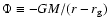 .
Equations are made
dimensionless by using the Schwarzschild radius
and the speed of light as reference units, i.e.,
.
Equations are made
dimensionless by using the Schwarzschild radius
and the speed of light as reference units, i.e.,
 and
and
 .
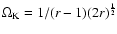
In these units, the Keplerian frequency is
denoted
.
In these units, the Keplerian frequency is
denoted
 .
In order to overcome the
technical difficulty of treating a realistic vertical structure,
three types of simplifying assumptions can be used; constant
thickness, constant angle (conical flows), or vertical equilibrium.
Chakrabarti & Das (2001) proved that
there is no essential difference among these three assumptions from
the point of view of the existence of stationary solutions.
The thickness of the flow is approximated as a
constant for the sake of
simplicity, as in Nakayama (1992), Nobuta & Hanawa (1994),
Blaes (1987) or MTK, although the approximate thickness
.
In order to overcome the
technical difficulty of treating a realistic vertical structure,
three types of simplifying assumptions can be used; constant
thickness, constant angle (conical flows), or vertical equilibrium.
Chakrabarti & Das (2001) proved that
there is no essential difference among these three assumptions from
the point of view of the existence of stationary solutions.
The thickness of the flow is approximated as a
constant for the sake of
simplicity, as in Nakayama (1992), Nobuta & Hanawa (1994),
Blaes (1987) or MTK, although the approximate thickness
 deduced from the balance of the vertical
pressure force and the vertical gravity is not constant.
deduced from the balance of the vertical
pressure force and the vertical gravity is not constant.
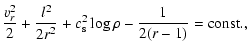
The stationary flow is described by the conservation of mass and the
Bernoulli equation:
 is the density,
 is the radial velocity,
 is the sound speed, and l is the specific angular momentum.
An example solution of unperturbed flow is shown in Fig. 1,
for which l=1.87 and
.
As a consequence of the inviscid hypothesis, stationary accretion
flows onto a black hole are very sub-Keplerian in their outer parts.
The question of the origin of this sub-Keplerian flow is still uncertain
(Chakrabarti & Titarchuk 1995; Molteni et al. 2001).
In Fig. 1, the unperturbed flow
is supersonic between the outer sonic point (
is the sound speed, and l is the specific angular momentum.
An example solution of unperturbed flow is shown in Fig. 1,
for which l=1.87 and
.
As a consequence of the inviscid hypothesis, stationary accretion
flows onto a black hole are very sub-Keplerian in their outer parts.
The question of the origin of this sub-Keplerian flow is still uncertain
(Chakrabarti & Titarchuk 1995; Molteni et al. 2001).
In Fig. 1, the unperturbed flow
is supersonic between the outer sonic point (
 )
and
the shock (
), becomes subsonic
between the shock and the inner sonic point (
)
and
the shock (
), becomes subsonic
between the shock and the inner sonic point (
 )
and goes into
the central black hole supersonically. This example solution is
precisely the one chosen by
Nobuta & Hanawa (1994), in which they showed that the outer shock is stable
to axisymmetric perturbations. Our numerical results in Sect. 3,
however, indicate that it is unstable to non-axisymmetric perturbations.
)
and goes into
the central black hole supersonically. This example solution is
precisely the one chosen by
Nobuta & Hanawa (1994), in which they showed that the outer shock is stable
to axisymmetric perturbations. Our numerical results in Sect. 3,
however, indicate that it is unstable to non-axisymmetric perturbations.
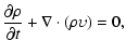
The mass conservation equation and the Euler equation are
written as follows:
 of the perturbation measured in the rotating
frame is defined as:
of the perturbation measured in the rotating
frame is defined as:
 |
(7) |
 is
the angular velocity.
With the standard method of linear stability analysis, (perturbations
proportional to e
is
the angular velocity.
With the standard method of linear stability analysis, (perturbations
proportional to e
 ,
see Appendix B), the
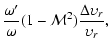
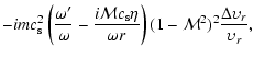
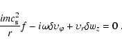
following differential system is obtained:
,
see Appendix B), the
following differential system is obtained:
 ,
wz is the vorticity along the rotation axis,
,
wz is the vorticity along the rotation axis,
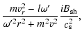
 is the radial Mach number, and the
subscript "sh'' denotes the shock position.
The boundary conditions corresponding to a perturbed shock velocity
is the radial Mach number, and the
subscript "sh'' denotes the shock position.
The boundary conditions corresponding to a perturbed shock velocity
 are obtained in Appendix C:
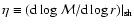 (Eq. (A.1)),
 and
are calculated at the post-shock side.
and
are calculated at the post-shock side.
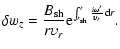
The
vorticity
 produced by the shock is:
 in our system, thus three boundary conditions are needed to solve
the equations. In addition to the two boundary conditions
Eqs. (10), (11)
at the shock, a third equation is obtained from the critical
condition at the sonic point,
.
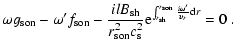
A single equation corresponding to this boundary value problem is
formulated in Appendix D.
in our system, thus three boundary conditions are needed to solve
the equations. In addition to the two boundary conditions
Eqs. (10), (11)
at the shock, a third equation is obtained from the critical
condition at the sonic point,
.
A single equation corresponding to this boundary value problem is
formulated in Appendix D.
![\begin{figure}
\par\includegraphics[width=8cm,clip]{3844f2.eps}\end{figure}](/articles/aa/full/2003/37/aa3844/img52.gif) |
Figure 2:
Eigenspectrum of the flow l=1.87 and
,
showing the instability
of the modes
 .
The empty triangles correspond to the stable
axisymmetric eigenmodes found by Nobuta & Hanawa (1994). .
The empty triangles correspond to the stable
axisymmetric eigenmodes found by Nobuta & Hanawa (1994).
|
| Open with DEXTER | |
![\begin{figure}
\par\includegraphics[width=8cm,clip]{3844f3.eps}\end{figure}](/articles/aa/full/2003/37/aa3844/img53.gif) |
Figure 3:
The maximum growth rate of the non radial modes is reached for  in the flow l=1.87 and
.
The pattern frequency in the flow l=1.87 and
.
The pattern frequency
 of
these unstable modes is concentrated in a limited band.
of
these unstable modes is concentrated in a limited band.
|
| Open with DEXTER | |
studied by Nobuta & Hanawa (1994),
for perturbations
 .
The stability of axisymmetric perturbations
confirms the results of Nobuta & Hanawa (1994).
In contrast, non-axisymmetric perturbations are unstable. The highest
growth rate is reached for m=10 perturbations, as seen in
Fig. 3. Determining numerically how the
most unstable m depends on the value of
.
The stability of axisymmetric perturbations
confirms the results of Nobuta & Hanawa (1994).
In contrast, non-axisymmetric perturbations are unstable. The highest
growth rate is reached for m=10 perturbations, as seen in
Fig. 3. Determining numerically how the
most unstable m depends on the value of
 is beyond the scope
of this paper.
In what follows, numerical calculations are restricted to m = 1perturbations for the sake of simplicity.
is beyond the scope
of this paper.
In what follows, numerical calculations are restricted to m = 1perturbations for the sake of simplicity.
![\begin{figure}
\par\includegraphics[width=8cm,clip]{3844f4.eps}\end{figure}](/articles/aa/full/2003/37/aa3844/img56.gif) |
Figure 4:
The two thick solid lines are the threshold for shock-included solutions.
The dotted lines measure the shock strength by the value of
 indicated on the left.
The thin solid lines correspond to the
value of the minimum
Mach number indicated on the left.
The thin solid lines correspond to the
value of the minimum
Mach number
 indicated on the
right.
The 19 filled circles correspond to unstable outer shock solutions, andthe
5 empty squares correspond to stable ones.
indicated on the
right.
The 19 filled circles correspond to unstable outer shock solutions, andthe
5 empty squares correspond to stable ones.
|
| Open with DEXTER | |
Figure 4 shows the domain
of angular momentum and sound
speed for which an isothermal inviscid flow, subsonic far from the
accretor, may accrete onto a black-hole through a stationary shock.
This domain is limited by two solid lines.
The solid line on the
left corresponds to the
solutions in which the inner shock and the outer shock are identical,
whereas the solid line on the right corresponds to
extremely weak shocks,
 .
A total of 24 shocked solutions were considered for numerical calculation,
in order to get a broad view of their stability properties.
Since the inner shock solution was already found
unstable to axisymmetric perturbations, we concentrated on the stability
of the outer shock solution. Solutions at the bottom right corner
in Fig. 4, for which the advection timescale is much longer
than the acoustic one (
.
A total of 24 shocked solutions were considered for numerical calculation,
in order to get a broad view of their stability properties.
Since the inner shock solution was already found
unstable to axisymmetric perturbations, we concentrated on the stability
of the outer shock solution. Solutions at the bottom right corner
in Fig. 4, for which the advection timescale is much longer
than the acoustic one (
 ),
were avoided for computing time reasons.
Among this sample of 24 shocked flows, 19 were found to be unstable and 5
to be stable. The results shown in Fig. 4 suggest that the
shock is generally unstable to non-axisymmetric perturbations, except
for a very narrow region close to the upper right border. In other words,
the shock might be stable only for
.
),
were avoided for computing time reasons.
Among this sample of 24 shocked flows, 19 were found to be unstable and 5
to be stable. The results shown in Fig. 4 suggest that the
shock is generally unstable to non-axisymmetric perturbations, except
for a very narrow region close to the upper right border. In other words,
the shock might be stable only for
.
![\begin{figure}
\par\includegraphics[width=8cm,clip]{3844f5.eps}\end{figure}](/articles/aa/full/2003/37/aa3844/img59.gif) |
Figure 5:
Growth rates compared to three timescales: advection
 (squares), acoustic
 (circles), and
rotation
(circles), and
rotation
 (crosses).
|
| Open with DEXTER | |
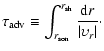
 ,
with a growth time comparable to the advection timescale
:
,
with a growth time comparable to the advection timescale
:
 |
(15) |
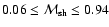
(i) the flow is generally unstable to non-axisymmetric perturbations,
even for mild shocks: the range of shock strengths among the 19unstable flows considered is very wide (
 ).
).
(ii) the growth time can be much shorter than the advection time.
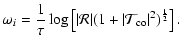
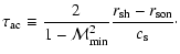
The growth time of the instability is plotted in Fig. 5,
in units of the rotation frequency at the sonic radius
,
the advection time
and also in units of
the acoustic time
approximated by the following lower bound:
 |
(16) |
The corotation radius
 of the perturbation is defined by
 ,
where
,
where
 :
:
 |
(17) |
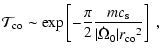
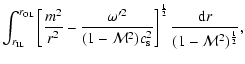
 ). The PPI is based on the exchange of energy
and angular momentum between acoustic waves propagating inside and
those propagating outside the corotation radius (Mark 1976).
The thin disc hypothesis in these studies is technically important in
order to treat high frequency perturbations in the WKB approximation
). The PPI is based on the exchange of energy
and angular momentum between acoustic waves propagating inside and
those propagating outside the corotation radius (Mark 1976).
The thin disc hypothesis in these studies is technically important in
order to treat high frequency perturbations in the WKB approximation
 .
According to Fig. 7, the high
frequency approximation is applicable only in the limit
.
According to Fig. 7, the high
frequency approximation is applicable only in the limit
 ,
which coincides with strong shocks according to Fig. 4.
Following GN85 and Kato (1987), we believe that
the physical mechanism captured analytically in thin discs is also
relevant in thicker discs (
,
which coincides with strong shocks according to Fig. 4.
Following GN85 and Kato (1987), we believe that
the physical mechanism captured analytically in thin discs is also
relevant in thicker discs (
 ), even if a
quantitative estimate of the growth rate is precluded.
), even if a
quantitative estimate of the growth rate is precluded.
![\begin{figure}
\par\includegraphics[width=8cm,clip]{3844f6.eps}\end{figure}](/articles/aa/full/2003/37/aa3844/img72.gif) |
Figure 6: The position of the corotation radius is indicated for 19 unstable flows (circles) and 5 stable ones (squares). |
| Open with DEXTER | |
![\begin{figure}
\par\includegraphics[width=8cm,clip]{3844f7.eps}\end{figure}](/articles/aa/full/2003/37/aa3844/img73.gif) |
Figure 7:
The value of the ratio
 at the sonic point
(dotted lines) and at the shock (full lines) is indicated on the
lines.
at the sonic point
(dotted lines) and at the shock (full lines) is indicated on the
lines.
|
| Open with DEXTER | |
The PPI
occurs with either an inner or an outer reflecting boundary, or even
more efficiently with both. Let us recall this mechanism in the case
of a single reflecting boundary, noting
 the
fractional amplitude of the transmitted wave through the corotation
zone, and
the
fractional amplitude of the transmitted wave through the corotation
zone, and  the fractional amplitude of the acoustic wave
reflected by the boundary. An incident wave with energy +1transmits an energy
the fractional amplitude of the acoustic wave
reflected by the boundary. An incident wave with energy +1transmits an energy
 on the other side of
corotation, thus amplifying the energy of the reflected wave by a
factor
on the other side of
corotation, thus amplifying the energy of the reflected wave by a
factor
 .
If
.
If  is the duration of the
acoustic cycle, the growth rate
is the duration of the
acoustic cycle, the growth rate  of this instability
is:
of this instability
is:
was obtained by GN85 and
confirmed by Kato (1987):
 ,
and the most
unstable modes correspond to
,
and the most
unstable modes correspond to
 .
Let us now
investigate the effects of radial advection on this
mechanism.
.
Let us now
investigate the effects of radial advection on this
mechanism.
The effect of advection on the corotation region can be
handled analytically in the high frequency limit.
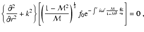
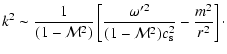
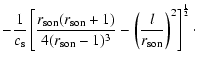
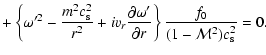
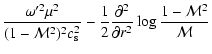
The second order
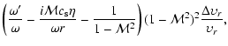
differential equation satisfied by the homogeneous solution f0 is
obtained in Appendix E:
 ), negative near the corotation radius
(
), negative near the corotation radius
(
 ),
and positive again at large radius. A calculation with
),
and positive again at large radius. A calculation with
 and
and
 in Appendix F
shows that
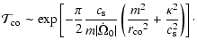
is
independent of the Mach number in the high frequency approximation,
if the gradient of the Mach number is neglected:
in Appendix F
shows that
is
independent of the Mach number in the high frequency approximation,
if the gradient of the Mach number is neglected:
 is the derivative of the rotation frequency at the
corotation radius.
This estimate at high frequency thus favours modes
with a low azimuthal number m. Beyond the high frequency
approximation, this calculation shows that the amplification
mechanism at corotation can operate even with radial
advection.
is the derivative of the rotation frequency at the
corotation radius.
This estimate at high frequency thus favours modes
with a low azimuthal number m. Beyond the high frequency
approximation, this calculation shows that the amplification
mechanism at corotation can operate even with radial
advection.
In order to estimate the effect of radial advection at
the inner boundary, Blaes (1987) considered
an inviscid flow with
constant thickness in a pseudo-Newtonian
potential, and a uniform angular momentum. It differed from the
present study by
an adiabatic hypothesis and, most importantly, a
leaking outer boundary.
As stressed by GN85, the PPI requires at
least one reflecting
boundary. The stabilizing effect of advection found by Blaes (1987)
is thus directly
related to the impossibility, for acoustic waves
moving away from the corotation,
to be reflected towards it.
By contrast, a stationary shock standing at the outer boundary of the flow
is a good reflector of acoustic waves, if the shock is not too weak.
A continuity argument would lead to expect the reflection coefficient
 to decrease to zero in the limit
 .
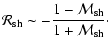
This is confirmed by a calculation of
in the
high frequency limit (see Appendix E), which gives the same result as
in isothermal flows without rotation (Foglizzo 2002):
.
This is confirmed by a calculation of
in the
high frequency limit (see Appendix E), which gives the same result as
in isothermal flows without rotation (Foglizzo 2002):
 )
is a sufficient condition for the instability of the
acoustic cycle between the shock and corotation in thin discs.
Acoustic energy in shocked flows is thus trapped between the shock
and the
corotation radius, and may leak inside through the sonic radius without
damping the instability.
On the basis of the results obtained by Blaes (1987), a strong decrease of
the growth rate should be expected in the weak shock limit.
This
trend is clear in Fig. 5, when measuring the growth
rate,
as Blaes (1987), in units of the rotation frequency at a fixed
radius.
What is more, all the stable modes correspond to weak shocks
(
)
is a sufficient condition for the instability of the
acoustic cycle between the shock and corotation in thin discs.
Acoustic energy in shocked flows is thus trapped between the shock
and the
corotation radius, and may leak inside through the sonic radius without
damping the instability.
On the basis of the results obtained by Blaes (1987), a strong decrease of
the growth rate should be expected in the weak shock limit.
This
trend is clear in Fig. 5, when measuring the growth
rate,
as Blaes (1987), in units of the rotation frequency at a fixed
radius.
What is more, all the stable modes correspond to weak shocks
(
 )
according to Fig. 6.
)
according to Fig. 6.
![\begin{figure}
\par\includegraphics[width=8cm,clip]{3844f8.eps}\end{figure}](/articles/aa/full/2003/37/aa3844/img97.gif) |
Figure 8:
Growth rate measured in units of the total acoustic time
(circles)
compared to the acoustic time
 between the corotation and the shock (stars). between the corotation and the shock (stars). |
| Open with DEXTER | |
Figure 8 shows that the dispersion of the points is
further decreased
by measuring the growth rate in units of the
acoustic timescale
between
the corotation and the
shock, approximated by:
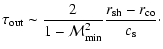
and strong shocks. A direct application of this
estimate outside its range of validity is unable to explain
the strong dispersion of the points in Fig. 8 for weak
shocks.
As noted in Sect. 4.2 with Fig. 7, solutions with a
weak shock coincides with those with the largest parameter
(
), i.e.the least adapted to a high frequency
approximation.
It should be noted that part of the dispersion of the
growth rate in Fig. 8 may come from the contribution of
the vorticity perturbations, when the advection time is comparable to
the acoustic time: they trigger additionnal acoustic waves which may
add or substract to the acoustic power present in the acoustic cycle.
Could this effect be essentially stabilizing? According to
Fig. 9, for a given shock strength (i.e.
 ), the flow seems to be stabilized by a strong advection.
![\begin{figure}
\par\includegraphics[width=8cm,clip]{3844f9.eps}\end{figure}](/articles/aa/full/2003/37/aa3844/img99.gif) |
Figure 9:
Incidence of advection on the PPI for weak shocks (
). The growth rate of the instability is measured in units of
the acoustic time
between the corotation and the
shock. |
| Open with DEXTER | |
Although
non-linear processes might redistribute the energy of the unstable
modes,
it could be tempting to identify the frequency
 ,
observed in the
simulations, with the real part of the most unstable eigenmode.
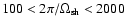
Based on five regular oscillation examples, MTK
found that the oscillation period P is always in the same range,
60 < P < 280 despite the large variation in the rotation rate at
the shock distance,
,
observed in the
simulations, with the real part of the most unstable eigenmode.
Based on five regular oscillation examples, MTK
found that the oscillation period P is always in the same range,
60 < P < 280 despite the large variation in the rotation rate at
the shock distance,
 .
We find that all the five regular oscillation examples listed in MTK satisfy
the condition,
.
We find that all the five regular oscillation examples listed in MTK satisfy
the condition,
 ,
which is a requirement of the PPI mechanism.
,
which is a requirement of the PPI mechanism.
A quantitative
comparison with the results of MTK is hampered by our
choice of an
isothermal flow rather than an adiabatic one, and also by our
restriction
to m=1 perturbations which are not necessarily the most
unstable ones.
A global understanding of which azimuthal wavenumber
corresponds to the
most unstable perturbation has not been reached yet.
The only isothermal example considered in Fig. 3 with m>1perturbations
favours
 ,
which seems higher than the low
azimuthal wavenumbers
present in the simulations of MTK.
,
which seems higher than the low
azimuthal wavenumbers
present in the simulations of MTK.
Despite these uncertainties, the present isothermal calculation
is simple
enough to illustrate the possibility of a PPI in a shocked accretion
flow, occuring on a shorter time scale than any possible
advective-acoustic cycle.
This instability mechanism should thus also apply to adiabatic flows,
including those simulated by MTK, if the shock is able to reflect
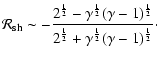
acoustic waves. The calculation of
in the
adiabatic hypothesis (Foglizzo & Tagger 2000, Eq. (C13)) would
be unchanged by rotation and non radial
perturbations, in the high frequency limit, for a strong shock:
 for
for
 ).
).
A refined comparison of the growth rate and
oscillation frequency with the results of MTK would require
a linear
stability analysis in an adiabatic flow involving also  perturbations.
This will be the subject of a forthcoming paper.
perturbations.
This will be the subject of a forthcoming paper.
The main results can be summarized as follows:
1. Despite post-shock deceleration, the outer shock solution is generally
unstable with respect to non-axisymmetric perturbations.
2. The growth time is comparable to the acoustic time if the shock
is not too weak. The flow might be stable only when
is
close to 1.
3. A WKB analysis of thin discs with advection
proves that the acoustic cycle between
the corotation radius and the
shock is unstable if the shock is strong, thus extending the
mechanism of the Papaloizou-Pringle instability to shocked discs
with advection.
4. Extrapolating the results established in thin
discs, the instability of thicker discs could be interpreted as a
form of the Papaloizou-Pringle instability modified by advection.
This interpretation is supported by the existence of a corotation
radius within the disc, a growth time comparable to the acoustic
time, and the role of the shock strength. The influence of advection
in the specific case of weak shocks, however, is still unexplained
(Fig. 9).
One particularity of this instability should be pointed out: although the instability mechanism relies on acoustic waves, vortical waves are continuously generated by the perturbed shock and advected to the accretor (Eqs. (12), (13)). These vortical waves (or the entropy/vorticity waves in the case of non isothermal flows) may play the role of the "blobs'' invoked frequently to model the time variability of X-ray binaries (e.g.references in Belloni et al. 2002). The observed properties of these blobs could therefore be used to test the validity of a model of shocked accretion.
Acknowledgements
The authors would like to thank Dr M. Tagger for discussions. W. Gu is grateful to Prof. Lu for his encouragement.
We consider a simple one-dimensional steady flow under the assumption
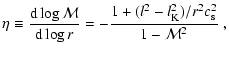
of a constant thickness. The derivative of the Mach number is
obtained
by derivating the stationary flow Eqs (1), (2):
 is the Keplerian angular momentum,
 .
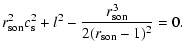
The continuity of the flow at the sonic point requires
.
The continuity of the flow at the sonic point requires
 |
(A.2) |
parameter space for the shocked accretion flows is shown
in Fig. 4.
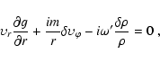
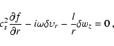
The mass conservation and Euler equations
are linearized in order to
obtain the following three equations:
 |
(B.1) |
 |
(B.2) |
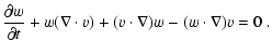 |
(B.4) |
 is related to f and
 (Eqs. (B.3), (13)),
 from (f,g).
The isothermal shock conditions are written as follows:
 |
(C.1) |
 |
(C.2) |
 |
(C.3) |
 in the radial
direction:
in the radial
direction:
 |
(C.4) |
 of the shock and its angle
 with the azimuthal direction are
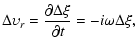 |
(C.5) |
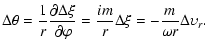 |
(C.6) |
 |
 |
(C.7) |
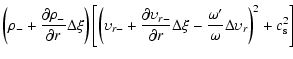  |
(C.8) |
 |
(C.9) |
With three boundary conditions
Eqs. (10), (11), (14), the differential
system
could in principle be
directly integrated using the Runge-Kutta method.
The singularity at the sonic point requires to integrate from the sonic
point towards the shock. The boundary value problem is conveniently
reduced to a
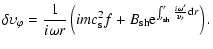
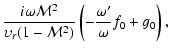
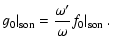
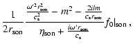
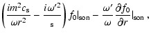
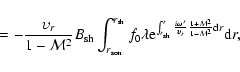
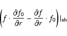
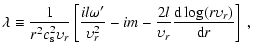
single equation involving the solution f0 of the homogeneous system.
The homogeneous differential equations are expressed as follows:
 |
(D.7) |
 is:
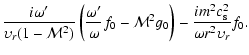
is:
 |
(D.9) |
 at the shock is deduced from Eqs. (8) and (10)-(12).
Perturbations
 at the
shock are decomposed on acoustic waves
at the
shock are decomposed on acoustic waves
 and
advected perturbations
and
advected perturbations
 :
:
 |
|||
 |
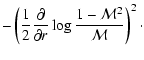
(E.3) |
| k2 |  |
 |
|
 |
(E.4) | ||
 |
|
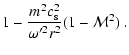 |
(E.5) |
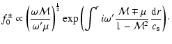
 are dominated by the phase variations in
the WKB limit:
are dominated by the phase variations in
the WKB limit:
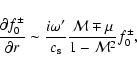 |
(E.8) |
 |
(E.9) |
 :
:
:
:
 |
(E.12) |
is defined using
Eq. (E.7), so that
 is the
fraction of the reflected acoustic flux reflected inward:
is the
fraction of the reflected acoustic flux reflected inward:
 |
|
 |
(E.13) |
| = | 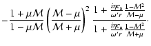 |
(E.14) |
 and the reflection coefficient is given by
Eq. (23).
and the reflection coefficient is given by
Eq. (23).
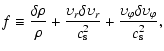
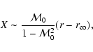
Defining a new variable X as in Foglizzo
(2001),
 |
(F.1) |
 |
(F.2) |
 |
(F.3) |
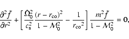 |
(F.4) |
by replacing the sound
speed
by
 ,
and the azimuthal
wavenumber m by
,
and the azimuthal
wavenumber m by
 .
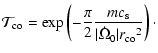
The fractional amplitude
of the transmitted wave, deduced from Eqs. (5)-(8) of GN85 is thus
independent of the Mach number in this approximation:
.
The fractional amplitude
of the transmitted wave, deduced from Eqs. (5)-(8) of GN85 is thus
independent of the Mach number in this approximation:
 |
(F.5) |
 the two zeros of kdeduced from Eq. (21),