![\begin{figure}
\par\includegraphics[width=7cm,clip]{3568_fig1.eps}
\end{figure}](/articles/aa/full/2003/37/aa3568/img19.gif) |
Figure 1:
a) Extraction of a sub-image (
|
| Open with DEXTER | |
In the text
![\begin{figure}
\par\includegraphics[width=5cm,clip]{3568_fig2.eps}
\end{figure}](/articles/aa/full/2003/37/aa3568/img41.gif) |
Figure 2:
Normalized PSF of the A370 image.
a) Contours Plot. The contours represent successively 100, 80, 60, 40, 20, 10, 5, 3.5, 2.5, 1.5, 0.8,
0.5, 0.2, 0.1 |
| Open with DEXTER | |
In the text
| |
Figure 3:
Relative error curve Rk between the CFHT reconstructed image and the HST one as a function of the iteration number for RL.
The images used are those of the Fig. 1, the PSF is the one of Fig. 2 and the mask used correspond to the rectangular box (
|
| Open with DEXTER | |
In the text
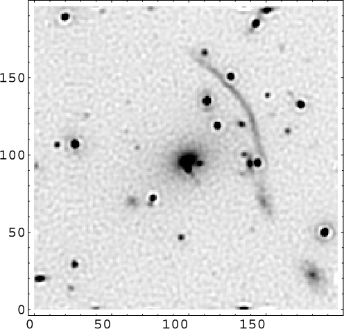 |
Figure 4:
Abell 370 reconstructed image by RL at the 50th iteration.
The image used is the one of Fig. 1a, the PSF is the one of Fig. 2 and the mask used correspond to the rectangular box (
|
| Open with DEXTER | |
In the text
| |
Figure 5:
Relative error curve Rk between the CFHT reconstructed image and the HST one as a function of the iteration number for LBCA.
The images used are those of the Fig. 1, the PSF is the one of Fig. 2 and the mask used correspond to the rectangular box (
|
| Open with DEXTER | |
In the text
![\begin{figure}
\par\includegraphics[width=7cm,clip]{3568_fig6.eps}
\end{figure}](/articles/aa/full/2003/37/aa3568/img51.gif) |
Figure 6: Best reconstructed image with LBCA using the HST reference image at the iteration 269. |
| Open with DEXTER | |
In the text
![\begin{figure}
\par\includegraphics[width=5cm,clip]{3568_fig7.eps}
\end{figure}](/articles/aa/full/2003/37/aa3568/img52.gif) |
Figure 7: Zoom on the radial arc R. HST image a), raw CFHT image b) and deconvolved CFHT image c). |
| Open with DEXTER | |
In the text
| |
Figure 8:
Relative error curve Ew(k) between the modulus of the FT of the reconstructed image at
iteration k (Abs
|
| Open with DEXTER | |
In the text
![\begin{figure}
\par\includegraphics[width=7cm,clip]{3568_fig9.eps}
\end{figure}](/articles/aa/full/2003/37/aa3568/img66.gif) |
Figure 9: Best reconstructed image with LBCA using a criterion based on the Wiener filter at the 129th iteration. |
| Open with DEXTER | |
In the text