A&A 408, 1057-1063 (2003)
DOI: 10.1051/0004-6361:20031028
S. A. Petrova
Institute of Radio Astronomy, 4, Chervonopraporna St., Kharkov 61002, Ukraine
Received 30 April 2003 / Accepted 3 June 2003
Abstract
Propagation of natural waves through the ultrarelativistic highly
magnetized plasma in the rotating magnetosphere of a pulsar is
considered. Based on the quantitative description of the
polarization-limiting effect, we develop a technique of density
diagnostics of pulsar plasma according to the observed
polarization profiles of radio pulses. For the first time, it
appears possible to obtain the profiles of the plasma density
distribution across the open field line tube. The density profiles
found for PSR B0355+54 and PSR B0628-28 show a perfect exponential
decrease towards the tube edge. The multiplicity factors derived
are compatible with those predicted by modern theories of pair
cascade in pulsars. The results of the plasma density diagnostics
may have numerous implications for the physics of the pulsar
magnetosphere. Further application of the suggested technique to
single-pulse polarization data seems to be promising.
Key words: plasmas - polarization - waves - stars: pulsars: general - stars: pulsars: individual: PSR B0355+54, PSR B0628-28
The diverse and complicated behaviour of the single pulse
polarization is mainly caused by the presence of orthogonal
polarization modes (OPMs), which are fundamental feature of
pulsar radiation. The concept of completely polarized superposed
OPMs has strong observational support (McKinnon & Stinebring
1998, 2000) and it is undoubtedly favoured by theoretical
considerations, since direct generation and further propagation of
the partially polarized disjoint modes are questionable. The
superposed modes can be recognized as the independently
propagating natural waves of pulsar plasma, which either are
generated by different emission mechanisms (McKinnon 1997) or
originate as a result of partial conversion of a single emission
mode (Petrova 2001). As the magnetic field of a pulsar is
extremely strong and ray propagation is typically
quasi-transverse, the natural waves of the magnetospheric plasma
should be linearly polarized, with the electric vector reflecting
the orientation of the ambient magnetic field. However, the
representation of the observed superposed OPMs as the natural
waves of pulsar plasma faces two major difficulties. Firstly, the
observed modes are elliptically polarized, with the degree of
circular polarization varying stochastically from pulse to pulse
(McKinnon 2002). Secondly, at a fixed pulse longitude, for each of
the orthogonal states there is a substantial pulse-to-pulse spread
in position angle (PA) of linear polarization (McKinnon &
Stinebring 1998), and moreover, the average PAs of the two states
may differ by not exactly ![]() (e.g. Gil et al. 1991, 1992).
(e.g. Gil et al. 1991, 1992).
From the theoretical point of view, if one consistently considers
propagation of natural waves in the open field line tube of a
pulsar, one cannot overlook the region where the waves decouple
from the magnetospheric plasma and become common vacuum
electromagnetic waves. This happens as soon as the plasma density
decreases sufficiently for the approximation of geometrical optics
to be broken, i.e. on condition that
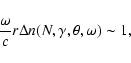 |
(1) |
In the present paper, we develop a technique that allows us to separate the observational consequences of PLE from the polarization data and to obtain the plasma number density profiles. The technique is applied to the average polarization profiles of PSR B0355+54 (at 4.85 GHz) and PSR B0628-28 (at 0.408 and 0.61 GHz), where the contribution of pulse-to-pulse orthogonal transitions is believed to be negligible, so that the average polarization characteristics can be regarded as those of a "typical'' single pulse. Although our results are rather illustrative, they do encourage further application of the suggested technique to real single pulses of a variety of pulsars, in which case the orthogonal transitions and other pulse-to-pulse polarization fluctuations can be properly taken into account. Our present research has made use of the database of published pulse profiles maintained by the European Pulsar Network, available at http://www.mpifr-bonn.mpg.de/pulsar/data.
| |
= | -2R(bx+ly)(by-lx)v, | |
| = | R[(bx+ly)2-(by-lx)2]v, | (2) | |
| = | 2R(bx+ly)(by-lx)q+R[(by-lx)2-(bx+ly)2]u, |
The Stokes parameters evolve along the wave trajectory because of
the plasma density decrease,
![]() ,
and also because
of variation of the orientation of the ambient magnetic field as a
result of ray propagation and pulsar rotation. For the wave
propagation far enough from the emission region, to the first
order in
,
and also because
of variation of the orientation of the ambient magnetic field as a
result of ray propagation and pulsar rotation. For the wave
propagation far enough from the emission region, to the first
order in
![]() (where
(where
![]() is the light cylinder
radius) the geometrical terms can be presented as (for more
details see e.g. Petrova & Lyubarskii 2000):
is the light cylinder
radius) the geometrical terms can be presented as (for more
details see e.g. Petrova & Lyubarskii 2000):
| bx+ly | = |  |
|
| by-lx | = | (3) |
Substituting Eq. (3) into Eq. (2), we find finally:
| |
= | ||
| = | (4) |
![\begin{displaymath}\frac{{\rm d}v}{{\rm d}w}=2\rho G_2(w-\rho G_1)Aq+[(\rho G_2)^2-(w-\rho
G_1)^2]Au.
\end{displaymath}](/articles/aa/full/2003/36/aa3917/img43.gif)
![\begin{displaymath}R(z_{\rm p})z_{\rm p}[(b_x+l_y)^2+(b_y-l_x)^2]_{z_{\rm p}}=1;
\end{displaymath}](/articles/aa/full/2003/36/aa3917/img45.gif) |
(5) |
| A | = | ![$\displaystyle \frac{w^3[(1-\rho G_1)^2+(\rho G_2)^2]}{[(w-\rho G_1)^2+(\rho
G_2...
...quad \rho=\frac{z_{\rm p}}{r_{\rm L}}\frac{\sin\alpha}{\vert\xi
-\alpha \vert},$](/articles/aa/full/2003/36/aa3917/img46.gif) |
|
| = |
The solution of the set of Eq. (4) at
![]() yields the
final polarization of the natural waves. Below we are interested
in the final degree of circular polarization,
yields the
final polarization of the natural waves. Below we are interested
in the final degree of circular polarization, ![]() ,
and the
final PA shift from the initial plane of magnetic lines,
,
and the
final PA shift from the initial plane of magnetic lines,
![]() .
Figure 1 shows the numerically calculated final polarization
characteristics of the ordinary waves as functions of the
parameters
.
Figure 1 shows the numerically calculated final polarization
characteristics of the ordinary waves as functions of the
parameters ![]() and
and ![]() .
According to Fig. 1c, the pairs
.
According to Fig. 1c, the pairs
![]() and
and
![]() exhibit a
unique correspondence.
exhibit a
unique correspondence.
![\begin{figure}
\includegraphics[width=8.8cm,clip]{3917f1a.eps}\par\includegraphi...
...ip]{3917f1b.eps}\par\includegraphics[width=8.8cm,clip]{3917f1c.eps} \end{figure}](/articles/aa/full/2003/36/aa3917/img57.gif) |
Figure 1:
The final ellipticity
a) and PA shift b) of the ordinary waves as
functions of parameters |
| Open with DEXTER | |
Both polarization characteristics of the natural waves, ![]() and
and
![]() ,
can be derived from observations. Given
that the observed radiation is an incoherent mixture of the
orthogonal elliptical modes with intensities I1 and I2, the
observed Stokes parameters (I, Q, U, V) are written as
,
can be derived from observations. Given
that the observed radiation is an incoherent mixture of the
orthogonal elliptical modes with intensities I1 and I2, the
observed Stokes parameters (I, Q, U, V) are written as
| I | = | ||
| V | = | vm(I1-I2), |
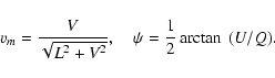 |
(6) |
| (7) |
![\begin{figure}
\includegraphics[width=8.8cm,clip]{3917f2.eps} \end{figure}](/articles/aa/full/2003/36/aa3917/img64.gif) |
Figure 2: Polarization profile of PSR B0355+54 at 4.85 GHz (von Hoensbroech & Xilouris 1997): solid line - total intensity, dashed line - linear polarization, dotted line - circular polarization, asterisks - reliable values of mode ellipticity. |
| Open with DEXTER | |
The profile of PSR B0355+54 is plotted in Fig. 2. The reliable
values of mode ellipticity, vm, calculated in accordance with
Eq. (6) are shown by asterisks. The errors in vm are assumed to
be normally distributed; hence, the standard error reads:
![]() where
where
![]() are the
rms-deviations of the Stokes parameters in the off-pulse region.
Our consideration involves the points with the relative errors
are the
rms-deviations of the Stokes parameters in the off-pulse region.
Our consideration involves the points with the relative errors
![]() .
The standard errors in PA,
.
The standard errors in PA,
![]() ,
and the
corresponding relative errors are typically much less.
,
and the
corresponding relative errors are typically much less.
![\begin{figure}
\includegraphics[width=8.8cm,clip]{3917f3.eps}\end{figure}](/articles/aa/full/2003/36/aa3917/img71.gif) |
Figure 3:
Parameter |
| Open with DEXTER | |
For the pulse longitudes considered, the tangent of the observed
PA is presented in Fig. 3 (triangles). According to the sign of the PA
derivative,
![]() .
Then, as can be seen from Eq. (4)
and Fig. 1, the negative sign of vm testifies to the dominance
of the ordinary waves. Using the numerical solution of
PLE-equations (4) at various
.
Then, as can be seen from Eq. (4)
and Fig. 1, the negative sign of vm testifies to the dominance
of the ordinary waves. Using the numerical solution of
PLE-equations (4) at various ![]() and
and ![]() ,
for each pair of
the observed values
,
for each pair of
the observed values
![]() one can find a unique pair
one can find a unique pair
![]() which provides such values of
which provides such values of ![]() and
and
![]() that satisfy both equalities (7)
simultaneously.
that satisfy both equalities (7)
simultaneously.
![\begin{figure}
\includegraphics[width=8.8cm,clip]{3917f4.eps}
\end{figure}](/articles/aa/full/2003/36/aa3917/img74.gif) |
Figure 4:
Parameter |
| Open with DEXTER | |
It should be mentioned that fitting the RVM-curve directly to the
observed PA usually faces difficulties, even in the absence of
prominent orthogonal transitions (e.g. Everett & Wiesberg 2001).
Moreover, in those rare cases when the fitting procedure yields
satisfactory results, the geometrical parameters of a pulsar
derived from the fitted curves at different frequencies appear to
differ drastically. Probably, these discrepancies can be
attributed to PLE. Further on it would be reasonable to allow for
this effect and fit the RVM-curve to ![]() rather than to
rather than to
![]() .
Although in the case considered,
.
Although in the case considered, ![]() and
and ![]() differ
slightly, in general one can expect that taking into account PLE
can improve the technique of RVM-fits, especially in application
to the single-pulse data.
differ
slightly, in general one can expect that taking into account PLE
can improve the technique of RVM-fits, especially in application
to the single-pulse data.
According to the theory of PLE, the linearly polarized natural
wave originating with the RVM position angle,
![]() ,
acquires both the observed
,
acquires both the observed ![]() and vmat a certain value of
and vmat a certain value of ![]() ,
which characterizes the physical
properties of the ambient plasma. The quantity
,
which characterizes the physical
properties of the ambient plasma. The quantity ![]() is related
to the polarization-limiting radius,
is related
to the polarization-limiting radius,
![]() ,
with
,
with
![]() .
In
our case C=2.3, corresponding to the slope of a straight line
in Fig. 3. Then
.
In
our case C=2.3, corresponding to the slope of a straight line
in Fig. 3. Then
![]() (cf. Fig. 4).
(cf. Fig. 4).
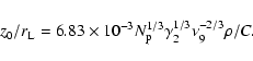
Proceeding from Eq. (5), one can find the plasma number density at
![]() :
:
![\begin{displaymath}N_{\rm p}=1.5\times 10^6P^{-1}\nu_9\gamma_2^2(\xi
-\alpha)^2C...
...^{-1}(1+\eta^2)
[(1-\rho G_1)^2+(\rho
G_2)^2]~~{\rm cm}^{-3},
\end{displaymath}](/articles/aa/full/2003/36/aa3917/img83.gif) |
(8) |
In view of the continuity of the plasma flow within the open field
line tube, it is convenient to introduce the multiplicity factor
of the plasma along a fixed field line,

 |
(9) |
The polar angle of the ray trajectory in the open field line tube,
![]() ,
can be expressed in terms of pulse phase of the ray along
with parameters of observational geometry. One can notice that far
from the emission region the radius-vector of the ray trajectory
makes approximately the same angle with the magnetic axis as does
the wavevector,
,
can be expressed in terms of pulse phase of the ray along
with parameters of observational geometry. One can notice that far
from the emission region the radius-vector of the ray trajectory
makes approximately the same angle with the magnetic axis as does
the wavevector,
![]() ,
where
,
where
![]() .
Hence, at the polarization-limiting radius,
.
Hence, at the polarization-limiting radius, ![]() ,
the
polar angle reads:
,
the
polar angle reads:
 |
(10) |
 |
(11) |
The dependence
![]() presents the plasma density
profile in the open field line tube. Although far from the
emission region, at
presents the plasma density
profile in the open field line tube. Although far from the
emission region, at
![]() ,
the tube is much wider than the
radio beam, it is still possible to probe the plasma density over
a substantial part of the tube. The point is that the
polarization-limiting radius can vary considerably across the
pulse profile (e.g., as in case of PSR B0355+54, see Fig. 4);
then, because of the magnetosphere rotation, for different rays
,
the tube is much wider than the
radio beam, it is still possible to probe the plasma density over
a substantial part of the tube. The point is that the
polarization-limiting radius can vary considerably across the
pulse profile (e.g., as in case of PSR B0355+54, see Fig. 4);
then, because of the magnetosphere rotation, for different rays
![]() can differ markedly (cf. Eq. (10)) and, in addition, for
distinct values of
can differ markedly (cf. Eq. (10)) and, in addition, for
distinct values of ![]() even close values of
even close values of
![]() may
correspond to distant field lines (cf. Eq. (11)).
may
correspond to distant field lines (cf. Eq. (11)).
Strictly speaking, the rays observed at different pulse longitudes
pass through the polarization-limiting region at different
azimuths, so that the plasma is probed only along the line
![]() .
However, if the azimuthal density
gradient is insignificant, one can suppose that
.
However, if the azimuthal density
gradient is insignificant, one can suppose that
![]() completely describes the plasma density distribution,
i.e. yields the density in any cross-section of the tube.
completely describes the plasma density distribution,
i.e. yields the density in any cross-section of the tube.
![\begin{figure}
\includegraphics[width=8.8cm,clip]{3917f5.eps}
\end{figure}](/articles/aa/full/2003/36/aa3917/img111.gif) |
Figure 5: Plasma density profiles of PSR B0355+54 (squares) and PSR B0628-28 (triangles and circles for the polarization data at 0.408 and 0.61 GHz, respectively). |
| Open with DEXTER | |
Substituting the calculated values of ![]() and
and ![]() into Eqs. (8)-(11),
we find the plasma density profile of PSR B0355+54
(squares in Fig. 5). Here it is taken that
into Eqs. (8)-(11),
we find the plasma density profile of PSR B0355+54
(squares in Fig. 5). Here it is taken that
![]() .
The dependence
.
The dependence
![]() exhibits a perfect exponential behaviour, with the exponent being
well fitted by polynomial of the second order. The values of
the multiplicity factor appear to be compatible with those given
by modern theories of pair cascade,
exhibits a perfect exponential behaviour, with the exponent being
well fitted by polynomial of the second order. The values of
the multiplicity factor appear to be compatible with those given
by modern theories of pair cascade,
![]() -100 (e.g.
Hibschman & Arons 2001a,b; Arendt & Eilek 2002). At the same
time, strong nonuniformity of the plasma distribution across the
tube is an essentially new result awaiting theoretical explanation.
-100 (e.g.
Hibschman & Arons 2001a,b; Arendt & Eilek 2002). At the same
time, strong nonuniformity of the plasma distribution across the
tube is an essentially new result awaiting theoretical explanation.
The suggested technique of plasma diagnostics has also been
applied to the polarization profiles of PSR B0628-28 at 0.408 and
0.61 GHz first published by Gould & Lyne (1998). The absence of
orthogonal transitions over a broad frequency range (Suleymanova
& Pugachev 2002) allows one to suppose that the average profiles of
PSR B0628-28 are appropriate for our treatment. The resultant
density profile is shown in Fig. 5 by triangles (0.408 GHz) and
circles (0.61 GHz) (it is taken that
![]() (Lyne
& Manchester 1988),
(Lyne
& Manchester 1988),
![]() ;
P=1.244 s,
;
P=1.244 s,
![]() ). One can see that the polarization data at
different frequencies lead to such multiplicity factors which
lie on the same curve, testifying to the validity of the suggested
technique. At the same time, this demonstrates that the
multifrequency polarization studies can extend the region suitable
for plasma probing, since the polarization-limiting radius is
frequency-dependent. Indeed, as the rays reach
). One can see that the polarization data at
different frequencies lead to such multiplicity factors which
lie on the same curve, testifying to the validity of the suggested
technique. At the same time, this demonstrates that the
multifrequency polarization studies can extend the region suitable
for plasma probing, since the polarization-limiting radius is
frequency-dependent. Indeed, as the rays reach
![]() ,
the
magnetosphere turns at an angle
,
the
magnetosphere turns at an angle ![]()
![]() ,
so
that the rays of different frequencies observed at the same pulse
longitudes probe the plasma at different field lines.
,
so
that the rays of different frequencies observed at the same pulse
longitudes probe the plasma at different field lines.
In the case of PSR B0628-28, the plasma multiplicity factor also shows
an exponential decrease, however, in contrast to the density
profile of PSR B0355+54, the second derivative of the exponent is
![]() 0, hinting at a flat maximum at smaller polar angles. Note
that in both density profiles, the main uncertainty comes
from the assumed values of
0, hinting at a flat maximum at smaller polar angles. Note
that in both density profiles, the main uncertainty comes
from the assumed values of
![]() .
As has already been
mentioned above, the customary RVM-fits usually yield questionable
results. Therefore the density profiles obtained perhaps appear
considerably shifted as a whole along both axes, though the
characteristic exponential form of
.
As has already been
mentioned above, the customary RVM-fits usually yield questionable
results. Therefore the density profiles obtained perhaps appear
considerably shifted as a whole along both axes, though the
characteristic exponential form of
![]() should
remain unaltered. The multiplicity factors derived are also
dependent on the assumed value of the characteristic
Lorentz-factor of the plasma particles (cf. Eqs. (8) and (9)).
Different models of the pair cascade certainly yield distinct
distribution functions of the secondary plasma and therefore the
characteristic Lorentz-factor should somewhat vary. However,
should
remain unaltered. The multiplicity factors derived are also
dependent on the assumed value of the characteristic
Lorentz-factor of the plasma particles (cf. Eqs. (8) and (9)).
Different models of the pair cascade certainly yield distinct
distribution functions of the secondary plasma and therefore the
characteristic Lorentz-factor should somewhat vary. However,
![]() is believed to be merely a scaling factor constant
throughout the pulse profile for a pulsar, so
that the shape of the density profile and its pulse-to-pulse
variations are not affected.
is believed to be merely a scaling factor constant
throughout the pulse profile for a pulsar, so
that the shape of the density profile and its pulse-to-pulse
variations are not affected.
The polarization profile of a pulsar at a fixed frequency typically does not allow one to reproduce the whole plasma density profile. Firstly, the rays propagating close enough to the magnetic axis remain invisible because of observational geometry. Secondly, far from the pulse profile peaks both V and L are too small to give reliable values of vm. Thirdly, the asymmetry of the observed total-intensity profiles may hint at a marked azimuthal dependence of the plasma density, in which case the polarization profile yields the multiplicity factor only along a line in the transverse cross-section of the tube. Note that joint observations at different frequencies can enlarge the region suitable for the plasma diagnostics, since the polarization-limiting radius is frequency-dependent.
The technique of plasma diagnostics has been applied to the average polarization profiles of PSR B0355+54 at 4.85 GHz and PSR B0628-28 at 0.408 and 0.61 GHz. The resultant multiplicity factors are compatible with those predicted by the modern theories of electron-positron cascade. In addition, we have found that the density distribution across the tube is essentially nonuniform, exhibiting a perfect exponential decrease towards the tube edge.
Since we have used the average polarization profiles in place of the singe-pulse ones, the results are expected to be rough. At the same time, they demonstrate the possibilities of the technique suggested and urge its further application to the single-pulse data. With the present level of observational facilities, it seems realistic to obtain the instanteneous plasma density profiles for a number of pulsars.
The plasma multiplicities and their variability, which is believed to underlie polarization fluctuations in single pulses, can impose constraints on the models of pair cascade and stimulate more detailed theoretical studies of the physics of the polar gap. Furthermore, explicit knowledge of the structure of the secondary plasma flow may provide new insights into emission physics of pulsars. At first, it would be interesting to compare the profiles of total intensity and plasma density as well as their temporal variations. In particular, the plasma diagnostics can help to find out whether the drifting and nulling phenomena are indeed associated with the spatial and temporal changes in the plasma density. A rigorous description of the density distribution of pulsar plasma can also provide a basis for quantitative studies of the propagation effects. For example, observational evidence for a non-uniformity of the plasma distribution across the tube confirms that refraction should be mainly determined by a transverse rather than radial density gradient, since the transverse scale length of the tube is much less. This strongly supports our model of refraction (see e.g. Petrova & Lyubarskii 2000), where the transverse density gradient was merely postulated. At the same time, the results of the present paper testify against the alternative model of refraction (e.g. McKinnon 1997) based on 'ducted' propagation of subluminal waves along the magnetic lines, since in the presence of a significant transverse density gradient this regime should be broken (Barnard & Arons 1986).
On the whole, the technique of plasma diagnostics suggested in the present paper can become a useful tool for studying the physics of the pulsar magnetosphere.
Acknowledgements
This research has made use of the polarization profiles from the database of the European Pulsar Network, which is operated by Max-Plank Institut fur Radioastronomie. I am grateful to the referee, A. Jessner, for useful comments and suggestions.