We report the first long-baseline interferometry of the circumstellar dust environment of R CrB. The observations were carried out with the Infrared Optical Telescope Array (IOTA), using our new
A&A 408, 553-558 (2003)
DOI: 10.1051/0004-6361:20031002
K. Ohnaka1 - U. Beckmann1 - J.-P. Berger2,3 - M. K. Brewer4 - K.-H. Hofmann1 - M. G. Lacasse2 - V. Malanushenko5 - R. Millan-Gabet2,6 - J. D. Monnier2,7 - E. Pedretti2 - D. Schertl1 - F. P. Schloerb4 - V. I. Shenavrin8 - W. A. Traub2 - G. Weigelt1 - B. F. Yudin8
1 -
Max-Planck-Institut für Radioastronomie,
Auf dem Hügel 69, 53121 Bonn, Germany
2 -
Harvard-Smithsonian Center for Astrophysics, 60 Garden Street,
Cambridge, MA 02138, USA
3 -
Laboratoire d'Astrophysique Observatoire de Grenoble,
Domaine Universitaire, 414 rue de la Piscine, BP 53,
38041 Grenoble Cedex 9, France
4 -
Department of Physics and Astronomy, University of Massachusetts,
Amherst, MA 01003, USA
5 -
Crimean Astrophysical Observatory, 98409 Crimea, Ukraine
6 -
California Institute of Technology, 770 S. Wilson Ave. MS 100-22,
Pasadena, CA 91125, USA
7 -
University of Michigan, 941 Dennison Building, 500 Church Street,
Ann Arbor, MI 48109-1090, USA
8 -
Sternberg Astronomical Institute, Universitetskii pr. 13, 119899 Moscow,
Russia
Received 28 March 2003 / Accepted 16 June 2003
Abstract
We report the first long-baseline interferometry of the circumstellar
dust environment of R CrB. The observations were carried out with the
Infrared Optical Telescope Array (IOTA), using our new
![]() beam combiner
which enables us to record fringes in the J, H, and
beam combiner
which enables us to record fringes in the J, H, and
![]() bands
simultaneously. The circumstellar dust envelope
of R CrB is resolved at a baseline of 21 m along a position angle of
bands
simultaneously. The circumstellar dust envelope
of R CrB is resolved at a baseline of 21 m along a position angle of
![]()
![]() ,
and the visibilities in the J, H, and
,
and the visibilities in the J, H, and
![]() bands
are
bands
are
![]() ,
,
![]() ,
and
,
and
![]() ,
respectively.
These observed visibilities, together with the
,
respectively.
These observed visibilities, together with the
![]() -band visibility
obtained by speckle interferometry with baselines of up to 6 m,
and the spectral energy distribution are compared with
predictions from spherical dust shell models which consist of the
central star and an optically thin dust shell.
The comparison reveals that the observed J- and H-band
visibilities are in agreement with those predicted by these
models, and the inner radius and inner boundary temperature
of the dust shell were derived to be 60-80
-band visibility
obtained by speckle interferometry with baselines of up to 6 m,
and the spectral energy distribution are compared with
predictions from spherical dust shell models which consist of the
central star and an optically thin dust shell.
The comparison reveals that the observed J- and H-band
visibilities are in agreement with those predicted by these
models, and the inner radius and inner boundary temperature
of the dust shell were derived to be 60-80 ![]() and 950-1050 K,
respectively.
However, the predicted
and 950-1050 K,
respectively.
However, the predicted
![]() -band visibilities are found to be
-band visibilities are found to be
![]() 10% smaller than the one obtained with IOTA.
Given the simplifications adopted in our models and
the complex nature of the object, this can nevertheless be regarded as rough
agreement. As a hypothesis to explain this small discrepancy,
we propose that there might be a group of newly formed dust clouds,
which may appear as a third visibility component.
10% smaller than the one obtained with IOTA.
Given the simplifications adopted in our models and
the complex nature of the object, this can nevertheless be regarded as rough
agreement. As a hypothesis to explain this small discrepancy,
we propose that there might be a group of newly formed dust clouds,
which may appear as a third visibility component.
Key words: techniques: interferometric - stars: circumstellar matter - stars: mass-loss - stars: individual: R CrB - stars: variable: general - infrared: stars
R Coronae Borealis (R CrB) stars are characterized by
irregular sudden declines in their visual light curves as deep as
![]() .
They are thought to undergo ejections of
dust clouds in random directions, and it is believed that
the sudden deep declines observed are a result of the
formation of dust clouds in the line of sight
(Loreta 1934; O'Keefe 1939).
However, the effective temperatures of R CrB stars are higher than
.
They are thought to undergo ejections of
dust clouds in random directions, and it is believed that
the sudden deep declines observed are a result of the
formation of dust clouds in the line of sight
(Loreta 1934; O'Keefe 1939).
However, the effective temperatures of R CrB stars are higher than
![]() 6000 K (Asplund et al. 2000),
and the mechanism of dust formation in such a hostile
environment is still unclear.
Particularly controversial is the location of the dust formation -
far from the star, at distances of
6000 K (Asplund et al. 2000),
and the mechanism of dust formation in such a hostile
environment is still unclear.
Particularly controversial is the location of the dust formation -
far from the star, at distances of ![]()
![]() (e.g. Fadeyev 1986,
1988; Feast 1996), or very close to the
photosphere, at
(e.g. Fadeyev 1986,
1988; Feast 1996), or very close to the
photosphere, at ![]()
![]() (Payne-Gaposchkin 1963).
R CrB stars have hydrogen-deficient and carbon-rich atmospheres
(e.g. Asplund et al. 2000), suggesting that they are
post-asymptotic giant branch stars. However, their
evolutionary status is little understood (see, e.g. Clayton
1996).
(Payne-Gaposchkin 1963).
R CrB stars have hydrogen-deficient and carbon-rich atmospheres
(e.g. Asplund et al. 2000), suggesting that they are
post-asymptotic giant branch stars. However, their
evolutionary status is little understood (see, e.g. Clayton
1996).
Ejected dust clouds are expected to be accelerated by radiation pressure. They absorb the starlight, re-emitting it in the infrared. Since R CrB stars are considered to undergo dust cloud ejections rather frequently, it is very likely that there is a group of dispersing dust clouds around the central star. No clear instantaneous correlation between the infrared and visual light curves is observed: the infrared light curves of R CrB stars do not exhibit a decline, even if the star undergoes a deep decline in the visual. Therefore, it is believed that a group of dispersing dust clouds, not one single, newly formed dust cloud, is responsible for the IR excess. Recently, Yudin et al. (2002) analyzed the infrared light curve of R CrB over 25 years and suggested that the IR excess increases with a time lag of about 4 years after the star undergoes decline events.
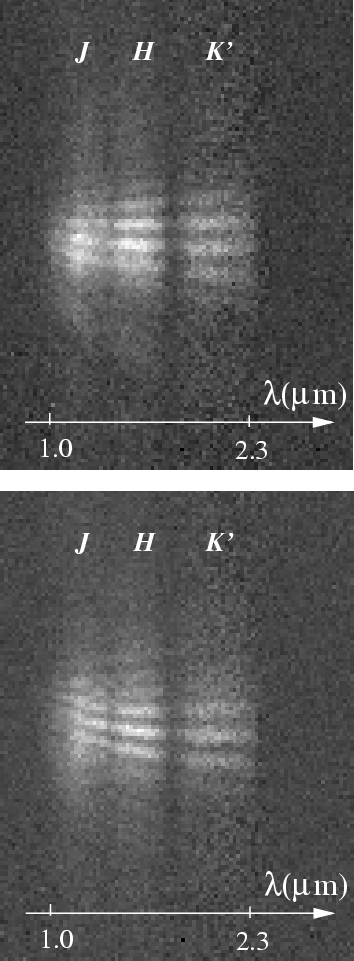 |
Figure 1:
Two consecutive interferograms of R CrB. The fringes are spectrally
dispersed in the horizontal direction and are recorded simultaneously
in the J, H, and
|
| Open with DEXTER | |
Our speckle interferometric
observations with a spatial resolution of 75 mas
have resolved the circumstellar envelope around R CrB
for the first time (Ohnaka et al. 2001, hereafter Paper I).
In Paper I, we show that simple, optically thin dust shell models can
simultaneously reproduce the visibility and
the spectral energy distribution (SED) obtained at near-maximum light
in 1996 and that the inner radius of the dust shell is
![]() 80
80 ![]() (19 mas) with a temperature of
(19 mas) with a temperature of ![]() 900 K.
Paper I also shows that
the visibility and SED obtained at minimum light in 1999 are not
in agreement with these models. As a possible interpretation,
the presence of a newly formed dust cloud was suggested,
but the spatial resolution of 75 mas was insufficient to
draw a clear conclusion about the presence of additional dust clouds.
900 K.
Paper I also shows that
the visibility and SED obtained at minimum light in 1999 are not
in agreement with these models. As a possible interpretation,
the presence of a newly formed dust cloud was suggested,
but the spatial resolution of 75 mas was insufficient to
draw a clear conclusion about the presence of additional dust clouds.
Long-baseline interferometry provides a unique opportunity to
investigate the circumstellar environment of R CrB stars with higher
spatial resolution. In this paper, we report the results of
observations of R CrB with the Infrared Optical Telescope Array (IOTA)
in the J, H, and
![]() bands.
We compare the observed SED and visibilities with those predicted
by the dust shell models which we used in Paper I and discuss
possible interpretations of the observed data.
bands.
We compare the observed SED and visibilities with those predicted
by the dust shell models which we used in Paper I and discuss
possible interpretations of the observed data.
Table 1:
IOTA observations for R CrB.
![]() :
projected baseline length,
PA: position angle of the projected baseline,
:
projected baseline length,
PA: position angle of the projected baseline,
![]() :
number of interferograms acquired for the target,
:
number of interferograms acquired for the target,
![]() :
number of interferograms acquired for the
reference star,
T: exposure time of each frame.
:
number of interferograms acquired for the
reference star,
T: exposure time of each frame.
The interferometric observations presented in this paper were
carried out with the IOTA interferometer (Traub 1998;
Traub et al. 2003)
on 2001 June 5 and 6. We used IOTA in the two-telescope
mode: a pair of 45 cm telescopes collect starlight and collimate it
into a pair of 4.5 cm beams, which are sent to the evacuated delay
line tubes. The outcoming beams are filtered through dichroics,
which feed the visible light onto star tracker CCDs and the infrared light
into our beam combiner. This latter consists of an anamorphic lens system,
a prism, and a HAWAII array detector (Weigelt et al. 2003a,b).
Spectrally dispersed fringes are
simultaneously recorded at all wavelengths in the range 1.0
to 2.3 ![]() m.
Figure 1 shows two examples of the interferograms
obtained for R CrB.
m.
Figure 1 shows two examples of the interferograms
obtained for R CrB.
Table 1 summarizes our observations of R CrB.
R CrB was at maximum light and had a visual magnitude of
approximately 6.
The observations were carried out with a baseline length of 21 m
along a position angle of ![]()
![]() on the sky.
on the sky.
The J-, H-, and
![]() -band visibilities of R CrB (= modulus
of the Fourier transform of the intensity distribution of the object)
were derived from the spectrally dispersed J-, H-, and
-band visibilities of R CrB (= modulus
of the Fourier transform of the intensity distribution of the object)
were derived from the spectrally dispersed J-, H-, and
![]() -band
Michelson interferograms. The data processing steps are described
in the Appendix A.
We derived the visibilities of R CrB to be
-band
Michelson interferograms. The data processing steps are described
in the Appendix A.
We derived the visibilities of R CrB to be
![]() ,
,
![]() ,
and
,
and
![]() in the J (wavelength range
1.04-1.44
in the J (wavelength range
1.04-1.44 ![]() m), H (1.46-1.84
m), H (1.46-1.84 ![]() m),
and
m),
and
![]() (1.94-2.30
(1.94-2.30 ![]() m) bands,
respectively. The corresponding mean spatial frequencies are
92.1 cycles/arcsec, 63.8 cycles/arcsec, and 48.8 cycles/arcsec
in the J, H, and
m) bands,
respectively. The corresponding mean spatial frequencies are
92.1 cycles/arcsec, 63.8 cycles/arcsec, and 48.8 cycles/arcsec
in the J, H, and
![]() bands, respectively.
bands, respectively.
The JHKLM photometric observations of R CrB were carried out on 2001 June 10 (only 5 days after the IOTA observations), using the 1.22 m telescope at the Crimean Laboratory of the Sternberg Astronomical Institute. UBV photometry was also carried out on the same night with the 1.25 m telescope at the Crimean Astrophysical Observatory.
The L- and M-band fluxes of R CrB vary semi-periodically on a time scale of 1260 days (Feast et al. 1997). At the time of our IOTA observations, R CrB was at maximum light in the visual as well as in the L band.
We first compare the observed SED and visibilities with
those predicted by the two-component models adopted in Paper I.
These two-component models consist of the central star and
a spherical, optically thin dust shell. Generally speaking,
it is difficult to examine such models and derive physical parameters
of the dust shell from observed SEDs alone.
However, observed visibilities can put
more constraints on the models and are therefore vital for testing models
as well as for deriving physical parameters.
Since the details of our model are described in Paper I, we only
give a summary here.
In the framework of our model, the circumstellar environment around
R CrB is represented by a spherical, optically thin dust shell of amorphous
carbon with a single grain size of 0.01 ![]() m, and
with density proportional to r-2.
The real circumstellar environment around R CrB is likely to be much
more complex. However, if dust ejection occurs frequently and in
random directions, such a simple, spherically symmetric shell model may be
regarded as an approximation of the complicated distribution of
material.
An effective temperature of 6750 K and a radius of 70
m, and
with density proportional to r-2.
The real circumstellar environment around R CrB is likely to be much
more complex. However, if dust ejection occurs frequently and in
random directions, such a simple, spherically symmetric shell model may be
regarded as an approximation of the complicated distribution of
material.
An effective temperature of 6750 K and a radius of 70 ![]() are adopted
for the central star, as described in Paper I.
The temperature distribution in the shell is calculated
from the thermal balance equation for an optically thin dust shell.
The input parameters of our model are the temperature
at the inner boundary and the optical depth of the dust shell.
We use the optical depth at 0.55
are adopted
for the central star, as described in Paper I.
The temperature distribution in the shell is calculated
from the thermal balance equation for an optically thin dust shell.
The input parameters of our model are the temperature
at the inner boundary and the optical depth of the dust shell.
We use the optical depth at 0.55 ![]() m as the reference optical
depth of the dust shell. At the time of our IOTA
observations, the star was at maximum light, and there were no obscuring
dust clouds in the line of sight. Therefore, unlike the studies presented in
Paper I, the empirical adoption
of extinction due to an obscuring dust cloud in front of the star
is not necessary here.
m as the reference optical
depth of the dust shell. At the time of our IOTA
observations, the star was at maximum light, and there were no obscuring
dust clouds in the line of sight. Therefore, unlike the studies presented in
Paper I, the empirical adoption
of extinction due to an obscuring dust cloud in front of the star
is not necessary here.
Figure 2a shows a comparison of
the observed SED and those predicted by the spherical
dust shell models.
Three different models are calculated with three different opacities
of amorphous carbon obtained by Bussoletti et al. (1987)
(AC2 sample),
Rouleau & Martin (1991) (AC1 sample), and Colangeli et al.
(1995) (ACAR sample).
The observed SED can be reproduced well with models
whose inner radius is 60-80 ![]() and inner boundary temperatures
are 950-1050 K.
The uncertainties of the inner temperature and inner radius are
estimated to be approximately
and inner boundary temperatures
are 950-1050 K.
The uncertainties of the inner temperature and inner radius are
estimated to be approximately ![]() 100 K and
100 K and ![]() 10
10 ![]() ,
respectively, for a given opacity data set.
,
respectively, for a given opacity data set.
![\begin{figure}
\par\resizebox{8.8cm}{!}{\rotatebox{0}{\includegraphics[bb=26 417...
...{\rotatebox{0}{\includegraphics[bb=26 28 544 350,clip]{3790F2.ps}}}
\end{figure}](/articles/aa/full/2003/35/aa3790/img27.gif) |
Figure 2:
Comparison of the observed SED and visibilities with
SEDs and visibilities
predicted by two-component models consisting of the central star and
an optically thin dust shell, as described in Sect. 4.1.
a) The filled circles represent the photometric data obtained
five days after the IOTA observations. The filled triangles represent
IRAS data.
The three curves represent models with different opacities for
amorphous carbon.
RM: Rouleau & Martin (1991),
CO: Colangeli et al. (1995),
BU: Bussoletti et al. (1987).
|
| Open with DEXTER | |
In Fig. 2b, we show a comparison of the J-, H-, and
![]() -band visibilities obtained with IOTA, together with the
-band visibilities obtained with IOTA, together with the
![]() -band speckle visibilities from Paper I, with those predicted from
the three models. It should be noted that these predicted visibilities are
calculated in the same manner as the observed
visibilities are derived (see Eq. (A.3)
in the Appendix A).
We also note that the
-band speckle visibilities from Paper I, with those predicted from
the three models. It should be noted that these predicted visibilities are
calculated in the same manner as the observed
visibilities are derived (see Eq. (A.3)
in the Appendix A).
We also note that the
![]() -band speckle visibilities obtained
at near-maximum light in 1996 and at minimum light
in 1999 show no significant difference within a cut-off frequency
of
-band speckle visibilities obtained
at near-maximum light in 1996 and at minimum light
in 1999 show no significant difference within a cut-off frequency
of ![]() 13 cycles/arcsec (see Fig. 2 in Paper I),
in spite of a brightness difference of 3.5 mag in the visual and
of
13 cycles/arcsec (see Fig. 2 in Paper I),
in spite of a brightness difference of 3.5 mag in the visual and
of ![]() 1 mag in the L and M bands.
Therefore, it would be reasonable
to use these speckle visibilities for the present study to cover
spatial frequencies smaller than 13 cycles/arcsec.
In the discussion here, we show only the visibilities obtained at
near-maximum light in 1996 for visual clarity.
Figure 2b shows that the three models can reproduce the
J- and H-band visibilities observed with IOTA, although
the predicted visibilities are somewhat higher in the H band.
1 mag in the L and M bands.
Therefore, it would be reasonable
to use these speckle visibilities for the present study to cover
spatial frequencies smaller than 13 cycles/arcsec.
In the discussion here, we show only the visibilities obtained at
near-maximum light in 1996 for visual clarity.
Figure 2b shows that the three models can reproduce the
J- and H-band visibilities observed with IOTA, although
the predicted visibilities are somewhat higher in the H band.
The high J-band visibility observed with IOTA suggests that
the contribution of the central star is dominant in the J band and
that the effect of scattering is small even in the J band, where
the contribution of scattered light is expected to be the largest
among the three bands. It suggests that the grain size in the dust
shell may be rather small.
This observational result is consistent with the result of the
simple analysis of the extinction curve of an obscuring dust cloud
in front of the star described in Paper I. In Paper I, we show that
the extinction curve of the obscuring dust cloud in the wavelength
region from the U to the I band can be approximated
as ![]()
![]() ,
and p changes from
,
and p changes from ![]() 0 to
0 to ![]() 1,
as the cloud disperses and becomes part of the optically thin dust shell
(see Fig. 5 of Paper I). Since the extinction
curve of amorphous carbon can be approximated by
1,
as the cloud disperses and becomes part of the optically thin dust shell
(see Fig. 5 of Paper I). Since the extinction
curve of amorphous carbon can be approximated by ![]()
![]() in the small particle limit (
in the small particle limit (
![]() ,
where a is the
radius of a spherical grain), the grain size is considered to be small
enough to fulfill the small particle limit in the UBVRI bands
when the cloud becomes part of the optically thin dust shell.
We can therefore estimate the size of grains in the optically thin
dust shell to be
,
where a is the
radius of a spherical grain), the grain size is considered to be small
enough to fulfill the small particle limit in the UBVRI bands
when the cloud becomes part of the optically thin dust shell.
We can therefore estimate the size of grains in the optically thin
dust shell to be ![]() 0.01
0.01 ![]() m, which satisfies
m, which satisfies
![]() for
for
![]()
![]() m.
With such small grains, the contribution of scattered light is
negligible, resulting in the high J-band visibility. This shows a
marked contrast with the case of HD 62623, where the observed J-band
visibility is lower than the H- and K-band visibilities, presumably
due to a presence of large grains (Bittar et al. 2001).
m.
With such small grains, the contribution of scattered light is
negligible, resulting in the high J-band visibility. This shows a
marked contrast with the case of HD 62623, where the observed J-band
visibility is lower than the H- and K-band visibilities, presumably
due to a presence of large grains (Bittar et al. 2001).
For the
![]() band, the predicted visibilities are
band, the predicted visibilities are ![]() 10%
lower than the visibility obtained with IOTA.
Given the complex nature of the circumstellar environment of
R CrB on the one hand and the simplifications adopted in our models on
the other hand, it is difficult to draw a definitive conclusion about
this discrepancy of
10%
lower than the visibility obtained with IOTA.
Given the complex nature of the circumstellar environment of
R CrB on the one hand and the simplifications adopted in our models on
the other hand, it is difficult to draw a definitive conclusion about
this discrepancy of ![]() 10%.
The small discrepancy may be due to a slight
deviation from spherical symmetry and/or to a presence of clumps,
which are plausible for R CrB.
10%.
The small discrepancy may be due to a slight
deviation from spherical symmetry and/or to a presence of clumps,
which are plausible for R CrB.
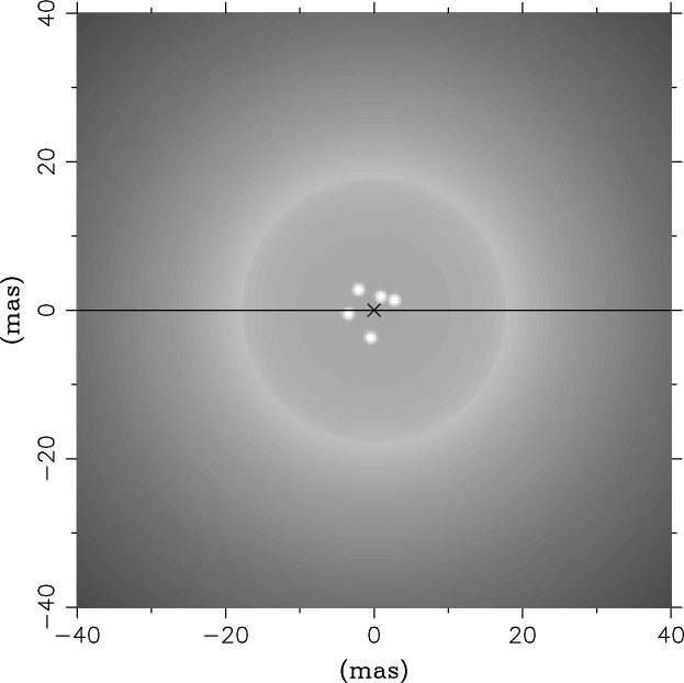 |
Figure 3:
An example of the intensity distribution of a model with
a group of dust clouds, which are randomly distributed at distances of
between 2 |
| Open with DEXTER | |
Alternatively, this small discrepancy can be interpreted as an
indication of the presence of an additional component, which is more
compact than the optically thin dust shell with the inner radius of
60-80 ![]() .
In fact, such a discrepancy
between observed visibilities and predictions from two-component
models had already been found in the study of the SED and
visibility obtained at minimum light (Paper I).
Although we tentatively assumed the presence of only one additional
obscuring dust cloud in Paper I, it seems to be more realistic to postulate
that there is probably a group of several newly formed dust clouds close to
the central star.
.
In fact, such a discrepancy
between observed visibilities and predictions from two-component
models had already been found in the study of the SED and
visibility obtained at minimum light (Paper I).
Although we tentatively assumed the presence of only one additional
obscuring dust cloud in Paper I, it seems to be more realistic to postulate
that there is probably a group of several newly formed dust clouds close to
the central star.
In order to see if such a picture is consistent
with the observed SED and visibilities, we constructed models with a
group of dust clouds, in addition to the extended optically thin dust shell.
We distributed a certain number of spherical dust clouds randomly
in the region between
![]() and
and ![]() .
All clouds are assumed to emit as a blackbody
of the same temperature and to have the same radius, which is
adjusted so that the total flux of the clouds, the optically
thin dust shell, and the central star is consistent with the observed SED.
Tentatively assuming a group of five clouds, we generated 10 random
distributions of hot dust clouds for a given set of
(
.
All clouds are assumed to emit as a blackbody
of the same temperature and to have the same radius, which is
adjusted so that the total flux of the clouds, the optically
thin dust shell, and the central star is consistent with the observed SED.
Tentatively assuming a group of five clouds, we generated 10 random
distributions of hot dust clouds for a given set of
(![]() ,
,
![]() ). We adopted a fixed value of 2
). We adopted a fixed value of 2 ![]() for
for
![]() and four different values of 10
and four different values of 10 ![]() ,
20
,
20 ![]() ,
30
,
30 ![]() ,
and 50
,
and 50 ![]() for
for ![]() .
An example of such models is shown in Fig. 3,
where a group of five intensity peaks resulting from hot dust clouds can be
seen together with the large limb-brightened, optically thin dust shell.
.
An example of such models is shown in Fig. 3,
where a group of five intensity peaks resulting from hot dust clouds can be
seen together with the large limb-brightened, optically thin dust shell.
Figure 4 shows a comparison of the observed SED and
visibilities with those predicted by
the models with five hot dust clouds out of the line of sight,
in addition to the optically thin dust shell discussed in
Sect. 4.1.
The parameters of the optically thin dust shell are the same or only slightly
changed, compared with those derived with the two-component models.
Figure 4b shows that the
![]() -band visibility observed with
IOTA is well reproduced by the models, while the agreement of the
H-band visibility is now slightly poorer than with the two-component
models. It is beyond the scope of the present work to
construct a more detailed model such as three-dimensional radiative
transfer models including dust formation processes, and we only suggest
here that the small discrepancy found in the
-band visibility observed with
IOTA is well reproduced by the models, while the agreement of the
H-band visibility is now slightly poorer than with the two-component
models. It is beyond the scope of the present work to
construct a more detailed model such as three-dimensional radiative
transfer models including dust formation processes, and we only suggest
here that the small discrepancy found in the
![]() -band visibilities may
be due to the presence of a group of newly formed hot dust clouds.
The temperature and
the size of the dust clouds are found to be approximately 1200 K and
2-3
-band visibilities may
be due to the presence of a group of newly formed hot dust clouds.
The temperature and
the size of the dust clouds are found to be approximately 1200 K and
2-3 ![]() ,
respectively.
We also calculated SEDs and visibilities
with a group of 10 clouds. However, as long as the radius of each cloud
is properly adjusted to reproduce the observed SED, the number of dust
clouds does not have a major effect on the resulting visibility
functions in the relevant spatial frequency range. The parameter
,
respectively.
We also calculated SEDs and visibilities
with a group of 10 clouds. However, as long as the radius of each cloud
is properly adjusted to reproduce the observed SED, the number of dust
clouds does not have a major effect on the resulting visibility
functions in the relevant spatial frequency range. The parameter
![]() does not have a huge influence on the resulting visibilities,
either. What matters is
the global extent of the group of dust clouds, namely
does not have a huge influence on the resulting visibilities,
either. What matters is
the global extent of the group of dust clouds, namely ![]() .
It turns out that
.
It turns out that
![]()
![]() can reproduce the
observed J-, H-, and
can reproduce the
observed J-, H-, and
![]() -band visibilities fairly well.
The adoption of smaller (
-band visibilities fairly well.
The adoption of smaller (
![]()
![]() )
or
larger (
)
or
larger (
![]()
![]() and
and ![]() 50
50 ![]() )
values
leads to poorer matches to the observed
)
values
leads to poorer matches to the observed
![]() -band visibility.
-band visibility.
![\begin{figure}
\par\resizebox{8.8cm}{!}{\rotatebox{0}{\includegraphics[bb=27 417...
...{\rotatebox{0}{\includegraphics[bb=26 27 543 347,clip]{3790F4.ps}}}
\end{figure}](/articles/aa/full/2003/35/aa3790/img42.gif) |
Figure 4: Comparison of the observed SED and visibilities with SEDs and visibilities predicted by models consisting of the central star, an optically thin dust shell, and a group of five newly formed dust clouds, as shown in Fig. 3. The dashed-dotted line in a) represents the contribution of the group of newly formed dust clouds in the RM model. See also the legend to Fig. 2. |
| Open with DEXTER | |
The first long-baseline interferometric observations of R CrB have
been carried out at the IOTA interferometer,
using our new
![]() beam combiner, which
enables us to record interferograms simultaneously in the J,
H, and
beam combiner, which
enables us to record interferograms simultaneously in the J,
H, and
![]() bands.
The J and H visibilities and the SED obtained
in the same period can be reproduced simultaneously by
two-component models consisting of the central star and an optically
thin dust shell with an inner radius of 60-80
bands.
The J and H visibilities and the SED obtained
in the same period can be reproduced simultaneously by
two-component models consisting of the central star and an optically
thin dust shell with an inner radius of 60-80 ![]() and
temperatures of 950-1050 K.
The
and
temperatures of 950-1050 K.
The
![]() -band visibilities predicted by these models are found to be
-band visibilities predicted by these models are found to be
![]() 10% lower than the observed
10% lower than the observed
![]() -band visibility.
It is possible to attribute this discrepancy to the simplifications
adopted in the two-component models. On the other hand,
we have also shown that
it may be due to the presence of a group of newly formed dust clouds
close to the central star. The observed visibilities and
SED can be reproduced simultaneously with such models, though not
perfectly, if such a group of dust clouds extends to a radius of
-band visibility.
It is possible to attribute this discrepancy to the simplifications
adopted in the two-component models. On the other hand,
we have also shown that
it may be due to the presence of a group of newly formed dust clouds
close to the central star. The observed visibilities and
SED can be reproduced simultaneously with such models, though not
perfectly, if such a group of dust clouds extends to a radius of
![]() 20
20 ![]() (
(![]() 5 mas),
with the temperature of each cloud
5 mas),
with the temperature of each cloud ![]() 1200 K.
1200 K.
The interferograms obtained with our
![]() beam combiner
are spectrally dispersed Michelson interferograms (see Fig. 1).
Each pixel column of the interferograms contains a one-dimensional
projection of the two-dimensional Michelson interferogram of a particular
spectral channel. The spectrally dispersed Michelson interferograms
cover the three near-infrared band passes J (1.04-1.44
beam combiner
are spectrally dispersed Michelson interferograms (see Fig. 1).
Each pixel column of the interferograms contains a one-dimensional
projection of the two-dimensional Michelson interferogram of a particular
spectral channel. The spectrally dispersed Michelson interferograms
cover the three near-infrared band passes J (1.04-1.44 ![]() m),
H (1.46-1.84
m),
H (1.46-1.84 ![]() m), and
m), and
![]() (1.94-2.30
(1.94-2.30 ![]() m).
The R CrB data consist of five pairs of the object and the reference star
data sets.
m).
The R CrB data consist of five pairs of the object and the reference star
data sets.
The derivation of the J-, H-, and
![]() -band visibilities
consists of the following image processing steps:
-band visibilities
consists of the following image processing steps:
(1) After flat-fielding, each interferogram
is processed in the following way: the power spectrum
(squared modulus of the Fourier transform) of the one-dimensional
Michelson interferogram of each spectral channel is calculated, and then
the average over all power spectra of all spectral channels within a
chosen wavelength region (e.g., J, H, or
![]() band) is
computed.
The resulting spectrally averaged power spectrum of an interferogram
consists of a central peak and two symmetric off-axis peaks.
band) is
computed.
The resulting spectrally averaged power spectrum of an interferogram
consists of a central peak and two symmetric off-axis peaks.
(2) Next, the detector and photon noise bias terms in each spectrally
averaged power spectrum are compensated.
(3) From this bias-compensated, spectrally averaged power spectrum,
the following squared raw visibility,
![]() or
or
![]() ,
is derived. The squared raw visibility
(
,
is derived. The squared raw visibility
(
![]() or
or
![]() )
is the
ratio of the integrated off-axis fringe peak intensity in the power
spectrum (= numerator of Eqs. (A.1) or (A.2)) and the
central peak intensity (= normalization integral in the denominator of
Eqs. (A.1) or (A.2)). The squared raw visibility
)
is the
ratio of the integrated off-axis fringe peak intensity in the power
spectrum (= numerator of Eqs. (A.1) or (A.2)) and the
central peak intensity (= normalization integral in the denominator of
Eqs. (A.1) or (A.2)). The squared raw visibility
![]() of an individual
interferogram of the object and the squared raw visibility
of an individual
interferogram of the object and the squared raw visibility
![]() of the reference star are given by
of the reference star are given by
 |
(A.4) |
 |
(A.5) |
The calibrated visibility
![]() obtained for the wavelength
interval from
obtained for the wavelength
interval from ![]() to
to ![]() is
assigned to the mean spatial frequency
is
assigned to the mean spatial frequency