A&A 406, 323-335 (2003)
DOI: 10.1051/0004-6361:20030492

CDS/SoHO multi-line observation of a solar active region: Detection of a hot stable loop and of a cool dynamic loop

S. Di Giorgio - F. Reale - G. Peres

Dipartimento di Scienze Fisiche ed Astronomiche, Università di Palermo, Sezione di Astronomia, Piazza del Parlamento 1, 90134 Palermo, Italy

Received 11 February 2002 / Accepted 28 March 2003

Abstract
We analyze a space-, time- and spectral-resolved SoHO/CDS observation of the evolution of an active region over a time lapse of approximately three hours in various spectral lines emitted in the interval of temperature $1.3 \times 10^4 < T < 2.5 \times 10^6$ K. We identify and characterize two structures of interest: a longer coronal loop ( ${\approx} 5.5\times10^9$ cm), relatively steady and well visible in lines forming at coronal temperatures (e.g. Fe XIV 334.17 Å, Fe XVI 360.76 Å) and a smaller one ( ${\approx} 1.8~\times~10^9$ cm), transient and visible only in cooler lines (O IV 554.51 Å, O V 629.73 Å). In the hot lines, the longer loop has a bright apex and an emission distribution of constant shape, but of moderately variable absolute intensity; the region around the loop apex shows a distinct brightening practically in all lines. In the hot lines, the brightening appears as a minor perturbation over a steadily high emission level. In the same region the emission measure vs temperature of the hottest lines indicates a temperature of $\sim$2 MK, lower than the temperature obtained from Yohkoh data taken just before the CDS observation. Comparison with steady-state loop scaling laws and with plasma time scales, and connection to cooling or heating episodes are discussed. As for the cool loop, its whole evolution, from ignition to disappearance, is directly observed, confirming the highly transient nature of such structures. The O V line is blue-shifted at one footpoint, indicating an upflow associated with the loop ignition.

Key words: Sun: UV radiation - Sun: transition region - Sun: corona - Sun: activity

   
1 Introduction

X-ray coronal loops are known to be stable on average over time scales longer than the characteristic cooling times of the plasma therein confined (e.g. Rosner et al. 1978), implying an "effectively continuous" heating source. The heating may be due to mechanisms such as the release of magnetic energy or dissipation of MHD waves, which may not occur constantly and uniformly in each loop. One basic question, therefore, concerns the time structure of the heating release: is the heating slowly varying or it consists of short, impulsive and intense episodes? A further question is whether the heat pulses occur continuously or there are preferential time scales and intensities (Litwin & Rosner 1993). In some well-studied cases, Yohkoh has shown flickering and variability of loop structures (e.g. Shimizu 1995) with characteristic time scales from 1 to 10 min. Wide-band soft X-ray observations cannot trace directly the heating pulses, because the detected brightenings are a consequence of highly non-linear effects: the increase of plasma emission measure coupled to the change of temperature that makes the plasma emit in different bands and intensity and be differently detected by the observing instrument.

The analysis of the time variations of the plasma emission is a necessary preliminary step to obtain information about the heating time structure. The response of the confined plasma depends on the heating characteristic times with respect to the plasma characteristic times (e.g. Reale & Peres 1995); for instance, we do not expect to observe significant emission variations if the heating pulses are very fast and frequent with respect to the plasma characteristic times (Peres et al. 1993). The compact and hot loop structures of active regions have small characteristic evolution times and allow more easily the detection of events on small time scales. The characteristic (thermodynamic) decay time, for instance, has been shown to scale as:

$$\tau_{\rm e} = 120 L_9/\sqrt{T_7}$$ (1)

where L₉ is the loop half length (in units of 10⁹ cm) and T₇is the loop maximum temperature (in units of 10⁷ K, Serio et al. 1991). This is confirmed by the observation of brightenings in loops (Shimizu 1995).

Observations in single coronal lines are more directly sensitive to plasma temperature variations; in particular, spatially resolved images, preferably at high time cadence, taken in spectral lines forming at different temperatures may provide better information on the heating time structure. This kind of observation can be accomplished with instruments on board SoHO.

This work is based on the data obtained in an approved SoHO Guest Investigation Program (GIP) aimed at investigating in detail the time structure of the heating episodes in solar active regions. The proposed observation considered CDS/NIS as leading instrument. The fundamental criteria to select the observation were: i) pointing to an active region, with a small field of view containing relatively small loops (length between 10 000 and 30 000 km), to be able to study individual loops well; ii) a time baseline long enough (few hours, at least) to be able to detect episodes on different time scales; iii) a sampling rate high enough to monitor rapid events, and constant to obtain homogeneous time sequences; iv) spatial resolution sufficient to study brightness distribution and to resolve loop structures; v) several spectral lines forming at different temperatures to cover thermal regimes from transition region to high corona. The selected lines cover a range $5.3 < \log (T) < 6.4$, with the addition of a chromospheric line (He I 584 Å, log (T)=4.3), taken for reference, and two very hot iron lines (Fe XXI and Fe XXII, $\log (T) \sim 7$), useful in case of very hot events.

The GIP was conducted in November 1997, and, in the present work, we present results of the analysis of the region thereby observed, including a few bright coronal structures. We analyze the morphology of the region and identify two well-defined bright loops, one hot and relatively long-lived, the other cool and transient. We analyze the time structure of the emission in several lines, deriving the characteristic time scales, discuss the correlations among the variations in different lines, the plasma physical conditions and the possible scenario.

In Sect. 2 we describe the observation, in Sect. 3 the analysis of the data, and in particular of those concerning the two loop structures, in Sect. 4 we discuss the data and draw our conclusions.

   
2 Observations

The Coronal Diagnostic Spectrometer (CDS) on board of SOlar Heliospheric Observatory (SoHO) is described in Harrison et al. (1995, 1997). It is composed by two distinct spectrometers: the Normal Incidence Spectrometer (NIS) and the Grazing Incidence Spectrometer (GIS). In this paper, we present data mainly from the CDS/NIS. The NIS gives simultaneously spatial information, along the slit, and spectral information. Images are obtained by rastering in the spatial direction perpendicular to the slit (here indicated as solar-x in agreement with the standard instrument notation). The NIS observes two spectral wavebands simultaneously: 308-381 Å with $\Delta\lambda\approx 0.08\$ Å (NIS1) and 512-633 Å with $\Delta\lambda\approx 0.14\$ Å (NIS2). It is not possible to take the entire spectrum of the NIS in one observation because of telemetry limitations, but smaller spectral windows can be selected. The choice of spectral windows depends on the particular solar feature to be studied.

Figure 1: Clockwise from the upper left. Yohkoh/SXT images (3 November 1997, 14:17 UT, Al.1 filter): full disk image, active region including the CDS field of view, CDS field of view; magnetogram of the CDS field of view (courtesy of NSO/Kitt Peak). The CDS field of view is marked in the two upper images. Contours of the O V line data (raster 8) are superposed on the magnetogram. The letters in the magnetogram mark the position of the footpoints of loops A and B. The color scale of the magnetogram ranges from -280 G (deep red) to 470 G (deep blue).

Open with DEXTER

Our observations consist of 14 rasters whose properties are given in Table 1. They begin at 21:18 UT of November 3 1997 and end at 00:12 UT of the following day. In the heliocentric system the coordinates of the center of the field of view are (785; 791) arcsec, at 21.31 UT.

Table 1: Properties of the CDS observation.

The width of a spectral pixel varies from 0.066 Å to 0.112 Å, depending on the spectral window. The raw data are available in 14 files, one per raster, written in standard FITS format. The first three rasters are taken 11.30 min from each other, the next ten at 13.20 min and the last is 9.20 min after the previous one. From now on we will refer to each raster by order number.

Within the standard CDS software, the raw data are de-biased to remove any electronic bias present in the data, cosmic rays are removed with the routine cds_clean_spike (Harrison et al. 1997), the data are calibrated with the routine nis_calib (September 21 1999 revision). Statistical uncertainties are extracted from photon counts. A correction for solar rotation is applied to the images.

Table 2 lists the ten lines that have been detected with significant S/N ratio, including the temperatures of maximum line emission. Spectroheliograms are obtained by integrating the spectra, the continuum subtracted.

Table 2: Detected lines in order of increasing temperature of peak emissivity.

	Figure 2: Top: sketch of the two loop structures identified in the CDS field of view. Bottom: two images of raster 8, clearly showing the two structures; left panel: the observation in the line of Fe XVI 360.76 Å; right panel: the one in the O V 629.73 Å line. The coordinates are in the heliocentric reference system. The gray scales are linear (for the extremes of the range see Fig. 3).
Open with DEXTER

   
3 Data analysis

3.1 Selected loops

The CDS field of view covers part of an active region. Figure 1 shows the full solar disc in the soft X-ray band [3-45] Å observed with the SXT on board of the satellite Yohkoh (pixel size $\approx$4.9 arcsec).

We analyze two loop structures observed with SoHO/CDS. Both structures are of interest because they are well identifiable and show brightness variability. Figure 2 includes a sketch of these structures in the field of view of the CDS. We have called loop A the more extended structure, the one also clearly visible in the SXT band (Fig. 1), and loop B the other one. Figure 3 shows an example of the images obtained with CDS in the ten spectral lines.

	Figure 3: Second CDS raster of the observed region in several continuum-subtracted lines. The images are ordered with increasing line-formation-temperature. $\lambda_{\min}=l$ and $\lambda_{\max}=L$ are the extremes of the integration in wavelength (Å) for each picture, m and M are the extremes of the linear grey scale (photons s-1 arcsec-2 cm-2).
Open with DEXTER

A first inspection of the temporal sequence of the images in each of the ten spectral lines provides the overall evolution of the region and of the two structures. In the hotter Fe XVI lines (see Fig. 2), as well as in the Yohkoh/SXT image (see Fig. 1), loop A is clearly visible and, as a first approximation, it is quite stable and stationary (at least in these hot lines). In the images taken in colder lines, the region is more inhomogeneous, with several irregular structures. The loop cannot be identified, except for its footpoints. This is in agreement with the standard scenario of coronal loops with the temperature maximum in the corona and temperature decreasing downwards to the transition region located in the footpoints. The images in the Mg VIII, Fe XII and Fe XIV lines clearly have lower signal to noise ratio.

In the O lines, loop B appears after raster 6. This loop is seen to evolve and finally to disappear and it isn't visible at all in the other lines. The evolution of this loop is shown in Fig. 4. Being invisible in the lines with $\log \ T > 5.9$, it is to be considered a "cold loop''. Loops like this are currently object of great interest (e.g. Brekke et al. 1997).

	Figure 4: Turn-on and -off of loop B in the O V 629 Å line, ( $\log T = 5.3$). Images are integrated in the band [628.69, 630.81] Å. Rasters are separated by 800 s. The upper left panel shows the entire loop at its maximum visibility (raster 8).
Open with DEXTER

   
3.2 Morphology of the structures

Most of loop A turns out to be visible in the hotter lines, but (what we presume to be) the feet of the structure are visible only in the colder lines. A localization of the bases of this loop from CDS data may be however quite difficult (and thus inaccurate). Loop A extends approximately from NW corner to slightly above the center of the observed region (see Fig. 2).

As for loop B, its SW footpoint is approximately at $x\sim1/3 \$ of image and $y \sim 2/3$; its NW footpoint is approximately at $x\sim 1/2 \$ of image and $y \sim 5/6 \$ (see also Fig. 2).

By comparing the CDS observations with a magnetogram of the photosphere below, we are more confident on the position of the footpoints of the loops. The magnetogram was obtained from the Nat. Solar Obs. at Kitt Peak, using the Fe line at $\lambda=8688.6$ Å (Table 3). The magnetogram has been superposed on CDS data as shown in Fig. 1, on the basis of the nominal sun-centered coordinates, corrected for the solar rotation due to the time delay between the magnetogram and the CDS data. CDS contour plots in O V line at various times have been superposed on the magnetogram. The O V contours encircle opposite magnetic poles that we associate to the footpoints of loop A. In the hotter Fe XVI lines, the most luminous region of loop A lies between the footpoints but it does not appear equidistant from them, rather closer to the SE footpoint. Finally a magnetic dipole can be associated to the footpoints of loop B well visible in raster 8 in the O lines. The comparison with the magnetogram suggests us that the two structures are magnetic tubes connecting regions of opposite polarity in the photosphere.

Table 3: Properties of magnetogram data (Data used are from NSO/Kitt Peak in cooperation with NSF/NOAO, NASA/GSFC, and NOAA/SEL.).

In order to estimate the physical dimensions of the loops we have assumed that they can be described as semicircular tubes with circular cross section. The diameter of each loop is the distance (in the magnetogram) between two points of opposite magnetic polarity in photosphere (points marked as A for loop A and B for loop B in Fig. 1), i.e. the footpoints. The lengths so found may underestimate the real ones, if, for instance, the loops were not perfectly semicircular, but quite stretched. The resulting total lengths of loop A and loop B are $5.5 \pm 0.4 \times 10^9$ cm and $1.8 \pm 0.2 \times 10^9$ cm, respectively.

3.3 Loop A

3.3.1 Loop luminosity profiles

	Figure 5: Loop A: sectors chosen to obtain the brightness profiles. Images are from raster 1.
Open with DEXTER

The profiles of luminosity along the loop have been extracted from the strip shown in Fig. 5. The strip has been divided into seven sectors. Profiles of sector average brightness are shown in Figs. 6 and 7, with the left end corresponding to the NW foot, averaging on several pixels ( ${\sim}20{-}30$) allows us to reduce the statistical errors. Here we have assumed that loop A is by far the brighest stucture along the line of sight. We neglected the effect of any background emission due to contributions from other unorganized structures intersecting along the line of sight. We have checked that the noise level, picked up in a dark region far from the loop but in the same field of view is small and constant (see Sect. 3.3.2).

Loop A can be identified in the lines with formation temperature $\log T \geq 5.9$. Figure 6 shows the profiles of luminosity along the loop for seven relevant lines in raster 3, each normalized to the respective maximum and shifted by an appropriate constant offset for the sake of clarity. Notice how the shape of the profiles changes from one line to the other: the profiles are concave in the cooler lines - Mg and Fe XII lines - but gradually become convex in the hot lines Fe XIV and Fe XVI. Notice also that the profiles are asymmetric, because of the orientation of the arc with respect to the line of sight. The brightest zone in the hot lines, probably the apex of the arc, is not in sector 3, but at the limit between sectors 4 and 5. The SE foot is more luminous that the other foot in all the lines.

We comment now the time variation of the profile shapes (and Fig. 7). In Fe lines the profiles appear quite steady with time, with few fluctuations, such as at rasters 9 and 10 in sector 1. The apex region is also quite stable, but significant variations are visible in Fe XVI, sector 4, around rasters 4, 12 and 13.

For a quantitative estimate of the amplitude of the variations, Fig. 8 shows profiles in two lines, with no offset. The relative variations are generally of the order of 10-20%, only larger in Fe XVI (25%-30%). We notice that in the cooler lines (up to Fe XII) the variations have random sign, as clear from the presence of numerous crossings between the profiles, and their amplitude is different from one sector to the other. In the hot Fe XVI line instead the variations are more coherent and systematic with time. A possible explanation for these differences between cold and hot lines is that, since the intermediate sectors of loop A are quite faint in the colder lines, emission from other - probably independent and uncorrelated - structures along the line of sight, clearly visible in Fig. 5 (Mg X line), becomes significant. The hot lines instead seem to detect only plasma confined in loop A, and therefore the evolution appears coherent along the loop. The coherent variations of luminosity along the loop are consistent with the characteristic times of propagation of thermal and hydrodynamic signals. In particular, the times of thermal conduction and sound propagation along all the arc at temperature of ${\sim} 2\times10^6$ K and density of ${\sim} 10^{10 }$ cm^-3 , are well below the temporal resolution of the observations.

   
3.3.2 Light curves

We have extracted the light curves in the selected lines in three zones of interest along the loop, each with an area of 16 pixels: at the two footpoints and in the region of maximum luminosity, that we believe to be close to the apex of the loop (see the Fig. 9). Figure 10 shows the light curves of the three zones in some lines. Also here, we take the line emission as coming entirely from the analyzed structure with no contamination from background structures along the line of sight. For reference, each panel shows a noise level, estimated as the emission averaged in a region of 21 pixels side located in the left-low part of the CDS field of view, where no bright structure is present in any selected line, and over all the rasters.

From a first inspection we note that spectral lines with similar formation temperatures have similar light curves in the same spatial zones. That is particularly evident, as an example, when comparing the light curves of the Fe XVI 335.41 Å line and of the Fe XVI 360.76 Å one.

Figure 6: Loop A: normalized profiles of luminosity along the loop, at a single time (raster 3) and for several lines. X-axis: coordinate along the loop from NW footpoint to SE footpoint; Y-axis: average intensity normalized to the maximum. For clarity's sake, the profiles are separated by an offset equal to 0.5. The lines are ordered from the bottom up with increasing temperature of line formation.

Open with DEXTER

Going into more details, we note that the region at the apex is by far the brightest one both in O lines and in Fe XVI line and remains the brightest during the whole observation. In the same lines, the S-E footpoint has intermediate luminosity and the other footpoint is instead the faintest region. In the other lines the differences of luminosity are smaller, and in Mg IX and Fe XII lines the light curves practically overlap. The Mg IX light curves are also much "flatter'' than the others, i.e. there is much less variability. In the other lines the evolution presents more distinct features. In particular, in all lines (except Mg IX) a brightening is visible at time $\sim$3000 s in the apex zone, followed by a high state, then a decay, then another rise. The initial brightening is more prominent in the O lines.

At the S-E zone, a first brightening appears too but delayed (by $\sim$1000 s) and fainter than the first brightening in the apex zone; a second brightening starts at $t \sim 7000$ s, is visible in all lines except Fe XVI (and Mg IX) and the emission remains high until the end of the observation. At the N-W zone the emission is invariably much more regular and, if any, shows a distinct decrease near the end of the observation, only in the Fe XIV and Fe XVI lines, clearly anticorrelated with the brightening at the S-E zone.

The fact that, at the apex, the brightening happens simultaneously in all the lines seems to indicate a coherent episode that involves plasma at various temperatures: an increase of temperature over a time smaller than the temporal resolution of the observation. Another possible explanation is the presence of another smaller structure that intersects loop A along the line of sight, and which interacts with loop A. The correlation and the delay observed at the SE foot seem to favor the former hypothesis and to indicate that the episode begins near the apex. The NW footpoint does not seem to be involved in this episode, probably both because it is not well enclosed in the selected zone, and because very distant from the other zones.

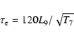
From the brightening and fading of the Fe XVI 360.76 Å line we have derived the characteristic times of the first impulse: the rise phase lasts $\sim$800 s (the time between two next rasters), the emission is then steady for $\sim$1600 s (two rasters) and decays in ${\approx} 2400$ s (three rasters). We can compare the decay time with characteristic loop cooling times: assuming a temperature $T_7 \approx 0.25$ and the length of loop A $L_{9} \approx 5.5$, the entropic decay time (Eq. (1)) is $\tau_{\rm e} \approx 1320$ s, the radiative cooling time is $\tau_{\rm r} \approx 6.7\tau_{\rm e}/T_7 \approx 35~000$ s and the conductive cooling time is $\tau_{\rm c} \approx 1.5\tau_{\rm e} \approx 2000$ s (Serio et al. 1991). We note that $\tau_{\rm e} \$ and $\tau_{\rm c}$ are not far from the observed decay time.

   
3.3.3 Physical conditions of the plasma

From the luminosity values of loop A we can estimate the temperature, density and pressure of the plasma confined in it.

Figure 11 shows the emission measure EM as a function of temperature, computed from the continuum-subtracted emission in the hottest lines (e.g. Jordan et al. 1987; Feldman et al. 1999) in the apex zone (see Fig. 9) in raster 4. The line emissivities are taken from database CHIANTI, and photospheric metal abundances (Dere et al. 1997) are assumed. We note that the various functions, in Fig. 11, almost intersect around the temperature of $2\times 10^6$ K, that, if the assumption of isothermal plasma holds, then yields the average temperature of the plasma confined in the loop A, a lower limit to its maximum temperature $T_{\max}$. From the same figure, it is possible to estimate the emission measure $EM \sim 5 \times 10^{46}$ cm^-3.

	Figure 7: Loop A: as in Fig. 6, but for all rasters and for three representative lines. For clarity's sake, the profiles are separated by an offset of 0.3.
Open with DEXTER

	Figure 8: Loop A: profiles of luminosity along the loop in two CDS lines analogous to those shown in Fig. 7, but with no offset and no normalization (the units are kphot s-1 cm-2 arcsec-2). Darker and darker lines correspond to progressively later times.
Open with DEXTER

	Figure 9: The boxes in the images mark the zones for which we have generated the light curves; the zones include also the solid borders.
Open with DEXTER

	Figure 10: Light curves of the apex ( squares), SE footpoint ( triangles) and NW footpoint. In each diagram the horizontal solid line marks the noise level.
Open with DEXTER

A range of plasma density $N_{\rm e}$ can be estimated with two extreme assumptions for the volume of the emitting plasma along the line of sight at the apex zone: one is a column with the apex zone as base area and the distance of the apex from the solar surface as height ( $h_{\rm A}\approx1.75\times10^9$ cm); the other is a cylinder with diameter and height equal to the width of the loop and the zone side (7 pixels), respectively. The former value is an upper limit for the volume. We find a density between ${\sim} 6\times10^{9}$ cm^-3 and ${\sim}9\times10^{9}$ cm^-3, corresponding to a pressure ( $2 N_{\rm e} k T$) between 3 and 5 dyne cm^-2.

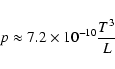
On the other hand, if the loop is close to, and fluctuates around, equilibrium conditions, the plasma pressure may be also estimated from the RTV (Rosner et al. 1978) scaling laws:

$$p \approx 7.2\times10^{-10}\frac{T^3}{L}$$ (2)

obtaining $p\approx 1$ dyne cm^-2 (assuming T = 2 MK) which is significantly less than what derived from the emission measure. We have several options to explain such a discrepancy:

• the presence of other structures along the line of sight may contribute to overestimate the density;
• element abundances higher than supposed would also lead to overestimate the density;
• the loop plasma may be very dynamic and variable, and the loop out of equilibrium (i.e. Eq. (2) may not hold);
• lack of ionization equilibrium may affect the density estimate in a non-trivial way;
• multi-thermal structure may lead us to underestimate the plasma temperature.

In order to check for the presence of hotter plasma components, we have analyzed Yohkoh/SXT data got just before the CDS observation (between 20:39 and 21:04 UT of 3 November 1997). We have identified loop A, and sectioned it into four sectors (each sector of $\approx$20 pixels). The temperature of the sector at the loop apex derived from Yohkoh/SXT filter ratios is $T= 4.0\pm 0.4$ MK, significantly higher than the temperature estimated from CDS data (Fig. 11), but with a lower emission measure ( ${\sim} 3 \times 10^{45}$ cm^-3), and leading to $p \approx 9$ dyne cm^-2, from RTV scaling law (Eq. (2)).

3.4 Loop B

Loop B is wholly visible only in rasters 8 and 9 and in the two oxygen lines (Figs. 4 and 3). From this we deduce that:

a)

it is "a cool loop", at temperature well under 10⁶ K;

b)

it is a "dynamic and transient loop", that appears, evolves and disappears within the observation.

In particular, the O V line data (Fig. 4) show that:

1.

loop B is not visible until raster 6;

2.

its S-W foot is very luminous at raster 7;

3.

loop B is entirely visible at raster 8;

4.

it is still entirely visible at raster 9, but less luminous;

5.

it is no longer visible from raster 10 on.

The O IV line data show a similar behaviour. The aforesaid evolution suggests that the loop is illuminated by a plasma flow at $T \sim 10^5$ K, relatively dense, rising from the SW foot toward the other one, which fills the loop, increasing its emission measure and making it visible. The loop then becomes less luminous probably for effect of the cooling.

3.4.1 Initial phase

If plasma flows initially upwards from the S-W foot, we expect blue shifted O lines when only the S-W foot is visible (raster 7). As the loop appears wholly luminous after other $800\pm 30$ s, i.e. in raster 8, we can infer an average speed of the luminous front of $v_{\min}\approx (23\pm3)$ km s^-1. This is a lower limit because the loop could brighten in less than the 800 s which separate the two rasters. We have analyzed the spectrum of the O V 629 Å line at the S-W foot when only this is visible (raster 7) and compared it to spectrum integrated on all the field of view. This last one will be taken as reference at rest.

In order to estimate the line Doppler shift, we have performed a best fit of the observed line profiles with a Gaussian function plus a constant (the continuum):

$$y=y_0\ {\rm e}^{\left(\lambda-\overline{\lambda}\right)^2/2\sigma^2}+d$$

with a search of the minimum $\chi^2$ in the space of the four parameters y₀, $\overline{\lambda}$, $\sigma \$and d. The assumption that the shape of the line is Gaussian is generally valid for its central zone (Cowley 1970). Parameter $\overline{\lambda}$ yields the line centroid and the difference between the value of $\overline{\lambda}$ obtained for the foot of S-W and that for all the region gives the Doppler shift. The fitting results are shown in Table 4 and Fig. 12.

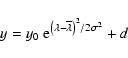
The blue-shift of the line centroid is $\Delta\lambda=(0.025\pm0.001)$ Å, corresponding to a speed along the line of sight of $(11.8\pm0.2)$ km s^-1. If it is assumed that the direction of the motion at the foot of the loop is radial with respect to the center of the Sun, taking into account the position of the region on the disc of the Sun, we obtain that the speed of the flow at the foot is $(21.9\pm0.4)$ km s^-1. This speed is well compatible with the lower limit of $\sim$23 km s^-1found previously on the base of purely geometric considerations and on the observed times. Therefore it is reasonable that the brightening of the loop is associated to this flow from the S-W foot. The sound speed at $2.4\times10^5$ K (the temperature of the maximum of emissivity of the O V line) is $v_{\rm s}\sim 80$ km s^-1, and the motion turns out to be largely subsonic.

Table 4: Parameters of the best fits of O V line profiles.

3.4.2 Cooling phase

Loop B fades between raster 8 and raster 9 and disappears between raster 9 and raster 10, i.e. the decay time interval is smaller than $\sim$1600 s. We can suppose that this decay is due to the cooling of the plasma confined inside the loop. If we assume that the arc, at the time of maximum luminosity (raster 8), is in nearly-stationary and hydrostatic conditions (albeit this hypothesis is not entirely justified), we find that the entropy decay time (Serio et al. 1991) of the loop is $\sim$800 s, compatible with the time in which the loop disappears.

   
4 Discussion and conclusions

In this work we have analyzed a space-, time- and spectral-resolved observation of the evolution of an active region in various spectral lines emitted in the temperature range $1.3 \times 10^4 < T < 2.5 \times 10^6$ K over a time lapse of approximately three hours. This observation was planned to yield detailed diagnostics of the variability and of the structuring of coronal loops, and, through them, of the evolution and structuring of the heating that makes them luminous. Our analysis has led us to identify and characterize two structures of interest: a longer coronal loop ( ${\approx} 5.5\times10^9$ cm), stationary and quite visible in lines forming at coronal temperatures, and a smaller one ( ${\approx} 1.8\times10^9$ cm), colder and transient.

The longer and hotter loop appears bright and well defined in the hot Fe ( $6.2 < \log T < 6.4$) lines; the apex region appears to be the brightest one and the luminosity to decrease to the footpoints. The loop appears less and less defined in cooler and cooler lines. In Mg lines of intermediate temperature ( $\log T \approx 6.0$) the loop region around the apex is fainter than the footpoints and in the oxygen cool lines ( $\log T \approx 5.3$) the loop is no longer visible as a whole, but only its footpoints. An inspection of the emission measure vs temperature of the hottest lines in the region of the apex indicates a temperature of $\sim$2 MK. Yohkoh data close in time to CDS data yield a temperature of $\sim$4 MK, well within the range of typical steady-state loops (Porter & Klimchuk 1995). This hotter plasma component may indicate a moderate multi-thermal structure along the line of sight, but, given the time interval between Yohkoh and CDS data, one cannot exclude that CDS may be detecting plasma slowly cooling from the hot condition seen in Yohkoh data. If taken as maximum loop temperature, the Yohkoh value makes pressure values obtained from scaling laws consistent with those implied by the plasma density obtained from CDS data. However, if CDS and Yohkoh were detecting the same plasma, we would expect comparable emission measures.

	Figure 11: Emission Measure (EM) versus temperature for the hottest lines. The value obtained from Yohkoh data is also shown ( square).
Open with DEXTER

	Figure 12: Loop B: Gaussian fit of spectral data relative to the O V line, normalized to the maxima of the fitting functions at time of raster 7. Data and the fitting of the spectrum of the entire field of view ( diamonds and solid line, respectively) and of the S-W footpoint of the loop ( squares, dashed line) are shown.
Open with DEXTER

Along the loop the emission in the cool lines appears to be more variable than in the hot lines. The variations at different positions along the loop are clearly correlated to each other in the hot lines, suggesting that in such lines we detect the evolution of plasma all contained in the loop. Episodes like the strong brightening in the O lines may resemble those analyzed by Chae et al. (2000) and interpreted as brightenings (or blinkers, e.g. Brekke 1999).

When analysing in detail the variability of different loop regions, the region around the loop apex appears to be the most variable. In particular, a distinct brightening occurs practically in all the lines, and it is more impulsive in the cool O lines, while more gradual and longer-lasting in the hot Fe lines. With the current time resolution it is hard to say whether the brightenings are correlated among the various lines. A strictly simultaneous event observed in several lines sensitive to plasma at different temperatures should imply that each line detects different plasma. An inspection of Fig. 9 seems to show that the brightening detected in O lines involves a structure different from loop A. We cannot exclude that the brightenings are originated from the interaction of different structures. The question is then whether the brightening detected in the hot lines is due to a heating or a cooling episode, i.e. a hot structure that, by cooling, becomes visible in the lines detected with CDS. The overdensity of the loop apex may indicate that the plasma involved in the brightening comes from a state of higher pressure, i.e. it is cooling. Figure 8 clearly shows that the whole loop is involved in coherent emission variations. The presence of a constant high emission level may then indicate that the cooling process involves only a fraction of the individual strands which the loop may consist of (see also Lenz et al. 1999). As mentioned above, some thermal structuring along the line of sight may be required also for consistency with Yohkoh data. An indication of thermal structuring along the line of sight in coronal loops has been shown recently using CDS data (Schmelz et al. 2001). One may also wonder whether the presence of such brightenings in the hot lines are somehow connected to the occurrence of distinct heating episodes: the so-called microflares. One should anyhow consider that the brightening episode appears as a perturbation over a stationary condition. Therefore, if microflares are indeed responsible of the loop heating they should be much more frequent than the episode observed here, since they should lead to a virtually constant, steady-state emission (Porter & Klimchuk 1995). Some preliminary results of hydrodynamic loop modeling seem to be in the same direction (Betta et al. 1999) but further investigation is needed.

Although the loop emission is not constant, the brightness variations are perturbations ($\sim$20% in the apex region in the Fe XVI line) over a steadily bright state. This makes this loop to resemble typical steady-state loops observed with Yohkoh, also in the light of the fact that small variations in plasma conditions are detected more easily in the CDS single line emission than in the Yohkoh broad band emission. The scenario coming from an overall inspection of the data for loop A is quite complex and the analysis presented here cannot be conclusive in this respect. More detailed observations, including simultaneous images at high time and space resolution such as those obtained with TRACE, may shed more light on the description of such coronal structures.

As for the cold loop, the existence of cold loops has been known for a long time (Foukal 1976) and SoHO has collected high-quality data showing the presence of dynamic cool loops (e.g. Brekke et al. 1997). The fact that they cannot be stable, rather dynamic and transient has been recently debated, but it is substantially based on the predictions of theoretical models (Peres 1999). What we observe here is clearly different from a simple blinker as those described in Brekke (1999), because here a whole cool loop clearly appears. The novelty of the present work is the direct observation and identification of the birth, evolution and cooling of one of such cool loops, bringing a direct confirmation of the highly transient nature of such structures. Moreover, we have identified a significant plasma flow from one footpoint to the other, clearly associated with the brightening evolution itself, and confirming that the motion of the bright front in the loop is due to plasma motion rather than heat propagation. Our analysis also shows that the decay of the loop may be instead due to the natural cooling of the plasma which has filled up the loop.

In summary, we may conclude that the interest of this work lies in particular in:

-

The study of the evolution of a coronal arc based on the analysis of lines with formation temperatures ranging from those typical of the transition region, to properly coronal values i.e. $T>2\times 10^6$ K.

-

The indication of coronal brightening episodes, somehow linked to heating and/or cooling processes, occurring in a loop already significantly bright in coronal lines.

-

The direct observation of the highly dynamic nature of a cold loop observed in the UV band and the relevant quantitative and self-consistent analysis of its evolution and dynamics.

In the spirit of the original observation program, this work is a preliminary step towards the detailed modeling and understanding of structures like the hot loop illustrated above, with the aid of time-dependent hydrodynamic codes describing plasma loop evolution (e.g. Peres et al. 1993; Betta et al. 1999).

Acknowledgements

The authors acknowledge support for this work from Agenzia Spaziale Italiana and Ministero dell'Università e della Ricerca Scientifica e Tecnologica. Data were collected in the course of the MEDOC campaign in November 1997. We acknowledge help of colleagues at MEDOC/IAS/Orsay and the warm atmosphere during the whole observing campaign.

References

 
• Betta, R. M., Peres, G., & Reale, F. 1999, in Plasma Dynamics and Diagnostics in the Solar Transition Region and Corona, SOHO 8th workshop, Paris 22-25 June 1999, ed. J.-C. Vial, & B. Kaldeich-Schuemann, ESA SP, 446, 179 In the text  
• Brekke, P. 1999, Sol. Phys., 190, 379 In the text NASA ADS  
• Brekke, P., Kjeldseth-Moe, O., & Harrison, R. A. 1997, Sol. Phys., 175, 511 In the text NASA ADS  
• Chae, J., Wang, H., Goode, P. R., et al. 2000, ApJ, 528, 119 In the text  
• Cowley, C. C. 1970, The theory of stellar spectra (New York: Gordon and Breach) In the text  
• Dere, K. P., Landi, E., Mason, H. P., et al. 1997, A&AS, 125, 149 In the text NASA ADS  
• Feldman, U., Doschek, G. A., Schüle, U., & Wilhelm, K. 1999, ApJ, 518, 500 In the text NASA ADS  
• Foukal, P. V. 1976, ApJ, 210, 575 In the text NASA ADS  
• Harrison, R. A., Fludra, A., Pike, C. D., et al. 1997, Sol. Phys., 4, 170, 123 In the text  
• Harrison, R. A., Sawyer, E. C., Carter, M. K., et al. 1995, Sol. Phys., 162, 233 In the text NASA ADS  
• Jordan, C., Ayres, T. R., Brown, A., Linsky, J. L., & Simon, T. 1987, MNRAS, 225, 903 In the text NASA ADS  
• Lenz, D. D., DeLuca, E. E., Golub, L., et al. 1999, Sol. Phys., 190, 131 In the text NASA ADS  
• Lin, R. P., Schwartz, R. A., Kane, S. R., et al. 1984, ApJ, 283, 421 NASA ADS  
• Litwin, C., & Rosner, R. 1993, ApJ, 412, 375 In the text NASA ADS  
• Peres, G., Reale, F., & Serio, S. 1993, in Physics of Solar and Coronae, ed. J. L. Linsky, & S. Serio (Kluwer Academic Pub.), 151 In the text  
• Peres, G. 1999, Proc. SoHO 8th workshop, Plasma Dynamics and Diagnostics in the Solar Transition Region and Corona, Paris 22-25 June 1999, ESA SP, 446, 43 In the text  
• Porter, L. J., & Klimchuk, J. A. 1995, ApJ, 454, 499 In the text NASA ADS  
• Reale, F., & Peres, G. 1995, A&A, 299, 225 In the text NASA ADS  
• Rosner, R., Tucker, W., & Vaiana, G. 1978, ApJ, 220, 643 In the text NASA ADS  
• Schadee, A., De Jager, C., & Svestka, Z. 1983, Sol. Phys., 89, 287 NASA ADS  
• Schmelz, J. T., Scopes, R. T., Cirtain, J. W., Winter, H. D., & Allen, J. D. 2001, ApJ, 556, 896 In the text NASA ADS  
• Serio, S., Reale, F., Jakimiec, J., et al. 1991, A&A, 241, 197 In the text NASA ADS  
• Shimizu, T. 1995, PASJ, 47, 251 In the text NASA ADS