![[*]](/icons/foot_motif.gif)
A&A 405, 821-831 (2003)
DOI: 10.1051/0004-6361:20030632
M. Einasto1 - J. Jaaniste1,2 - J. Einasto1 - P. Heinämäki1,3 - V. Müller4 - D. L. Tucker5
1 - Tartu Observatory, 61602 Tõravere, Estonia
2 -
Institute of Physics, Estonian Agricultural University,
Kreutzwaldi 64, 51014 Tartu, Estonia
3 -
Tuorla Observatory, Väisäläntie 20, Piikkiö, Finland
4 -
Astrophysical Institute Potsdam, An der Sternwarte 16,
14482 Potsdam, Germany
5 -
Fermi National Accelerator Laboratory, MS 127, PO Box 500, Batavia,
IL 60510, USA
Received 23 January 2003 / Accepted 17 April 2003
Abstract
We study the spatial distribution of loose groups from the Las Campanas
Redshift Survey, comparing it with the supercluster-void network
delineated by rich clusters of galaxies. We use density fields and
the friends-of-friends (FoF) algorithm to identify the members of
superclusters of Abell clusters among the Las Campanas loose groups.
We find that systems of loose groups tend
to be oriented perpendicularly to the
line-of-sight, and discuss possible reasons for that.
We show that loose groups in richer systems (superclusters
of Abell clusters) are themselves also richer and more massive than
groups in systems without Abell clusters. Our results indicate
that superclusters, as high density environments, have a major role in
the formation and evolution of galaxy systems.
Key words: cosmology: observations - cosmology: large-scale structure of the Universe
are the
largest relatively isolated density enhancements
in the Universe. As commonly
accepted, superclusters are formed by perturbations of the same
wavelength in the initial density field (Einasto et al. 2001
and references therein).
Superclusters have mainly been studied using the data on rich clusters of galaxies (Einasto et al. 2001, and references therein). Properties of superclusters (their shapes and orientations) have been studied by West (1989), Plionis et al. (1992), Jaaniste et al. (1998) and Kolokotronis et al. (2002). Already early studies of the fine structure of nearby superclusters and of the distribution of matter in low density regions between superclusters (Lindner et al. 1995 and references therein) showed that superclusters have a complicated structure, where clusters and groups of galaxies are connected by filaments of galaxies. Superclusters may also contain hot gas (Kull & Böhringer 1999; Bardelli et al. 2000; Rines et al. 2001; Rose et al. 2002).
At present several deep galaxy surveys are publicly available. Among these surveys are the ESO Slice Project survey (ESP, Vettolani et al. 1997), the Las Campanas Redshift Survey (LCRS; Shectman et al. 1996), the 2 degree Field Galaxy Redshift Survey (2dF, Colless et al. 2001) and the Sloan Digital Sky Survey (SDSS, York et al. 2000). These surveys can be used to study the structure of a large number of superclusters in more detail and on larger scales than hitherto possible.
The catalogue of loose groups of galaxies extracted from the LCRS
(LCLGs, Tucker et al. 2000, hereafter TUC) gives us
an opportunity to study the spatial distribution and intrinsic
properties of loose groups on large scales, up to redshifts
 .
In the LCRS, galaxies have been observed in 6 thin slices;
thus, in order to use this survey to study the 3D structure of
the Universe, it is necessary to analyse this survey together with data on
rich clusters of galaxies, e.g. Abell clusters.
Such a combined analysis of the spatial distribution of loose groups,
Abell clusters, and superclusters of Abell clusters enables us to
exploit the deep slices to study the fine structure of
superclusters and the hierarchy of the structures in the Universe.
.
In the LCRS, galaxies have been observed in 6 thin slices;
thus, in order to use this survey to study the 3D structure of
the Universe, it is necessary to analyse this survey together with data on
rich clusters of galaxies, e.g. Abell clusters.
Such a combined analysis of the spatial distribution of loose groups,
Abell clusters, and superclusters of Abell clusters enables us to
exploit the deep slices to study the fine structure of
superclusters and the hierarchy of the structures in the Universe.
In the present paper we found populations of LCLGs in superclusters of Abell clusters, using density fields and the friends-of-friends (FoF) analysis of the LCRS. We studied the properties of these systems and the distribution of LCLGs with respect to the supercluster-void network, traced by Abell clusters. We also studied the properties of LCLGs in systems that contain no Abell clusters.
In the next section we describe our LCLG and Abell cluster samples. In Sect. 3 we identify LCLGs that belong to superclusters. Then we study the properties of superclusters and the distribution of LCLGs with respect to the supercluster-void network. In the last two sections we give a discussion and summary of our results.
The LCRS (Shectman et al. 1996) is an optically selected
galaxy redshift survey that extends to a redshift of 0.2 and is
composed of six slices, each covering an area of roughly
 .
Three of these slices are located in the Northern
Galactic Cap and are centred at the declinations
.
Three of these slices are located in the Northern
Galactic Cap and are centred at the declinations
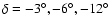 ;
the other three slices are located in the
Southern Galactic Cap and are centred at the declinations
;
the other three slices are located in the
Southern Galactic Cap and are centred at the declinations
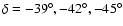 .
The thickness of slices is
approximately 7.5 h-1 Mpc at the survey's median redshift.
Altogether, the LCRS contains redshifts for 23 697 galaxies within
its official photometric and geometric boundaries.
.
The thickness of slices is
approximately 7.5 h-1 Mpc at the survey's median redshift.
Altogether, the LCRS contains redshifts for 23 697 galaxies within
its official photometric and geometric boundaries.
The survey spectroscopy was carried out using a 50 fibre multiobject
spectrograph with the nominal apparent magnitude limits
for the spectroscopic fields
 ,
and
a 112 fibre multiobject
spectrograph with a larger range of
apparent magnitudes (
,
and
a 112 fibre multiobject
spectrograph with a larger range of
apparent magnitudes (
 ).
Therefore, the selection criteria varied from field to
field, often within a given slice.
).
Therefore, the selection criteria varied from field to
field, often within a given slice.
Using the FoF percolation algorithm, TUC extracted the LCLG catalogue
from the LCRS. The linking lengths were chosen so that each
group is contained within a galaxy number density enhancement contour
of
 .
When extracting these LCLGs, great care was taken
to account for
the radial selection function, the
field-to-field selection effects inherent in the LCRS,
and the boundary effects due to the fact that the LCRS is
composed of six thin slices.
As the derived properties of the LCLGs in the 50-fibre
fields do not differ substantially from the derived properties of the
LCLGs in the 112-fibre fields, the selection effects were successfully
eliminated.
.
When extracting these LCLGs, great care was taken
to account for
the radial selection function, the
field-to-field selection effects inherent in the LCRS,
and the boundary effects due to the fact that the LCRS is
composed of six thin slices.
As the derived properties of the LCLGs in the 50-fibre
fields do not differ substantially from the derived properties of the
LCLGs in the 112-fibre fields, the selection effects were successfully
eliminated.
The LCLG catalogue contains 1495 groups in the redshift range of
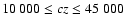 km s-1. This is one of the first deep,
wide samples of loose groups; as such, it enables us for the first
time to investigate the spatial distribution and properties of groups in
a large volume.
km s-1. This is one of the first deep,
wide samples of loose groups; as such, it enables us for the first
time to investigate the spatial distribution and properties of groups in
a large volume.
![\begin{figure}
\par\includegraphics[width=8.1cm,clip]{H4267F1.ps}\end{figure}](/articles/aa/full/2003/27/aah4267/img17.gif) |
Figure 1:
Multiplicity function of LCLGs showing the fraction of groups
in systems with at least 2 members as a function of the neighbourhood
radius. Bold lines: solid line - slice
 ,
dotted
line - slice ,
dotted
line - slice
 ,
dashed line - slice ,
dashed line - slice
 .
Thin lines: solid line: slice .
Thin lines: solid line: slice
 ,
dotted line - slice ,
dotted line - slice
 ,
and dashed line - slice ,
and dashed line - slice
 .
Note the difference between the slice
and other slices. .
Note the difference between the slice
and other slices. |
| Open with DEXTER | |
Einasto et al. (2001) identified superclusters of Abell clusters ("Abell superclusters'') using the FoF algorithm with linking the length R = 24 h-1 Mpc that corresponds approximately to an overdensity contour of 2. This radius was chosen by studying the spatial distribution of rich clusters of galaxies. This list helps us to identify Abell superclusters that cross the LCRS slices. Using the same linking length to search for members of superclusters among the loose groups links almost 90-95% of groups (Fig. 1). At the other extreme, by simply identifying as supercluster members those loose groups that are located around rich clusters in a sphere of radius R = 6 h-1 Mpc, as done by Einasto et al. (2003a), we miss the outer members of superclusters. Thus we have used additional methods to determine the system membership. We identified systems of loose groups and then searched for those systems that belong to Abell superclusters as described in the following two subsections.
To identify systems of loose groups we applied the FoF algorithm to LCLGs from the each Las Campanas slice separately using a wide range of linking lengths (or neighbourhood radii). Figure 1 shows the fraction of LCLGs in systems with at least 2 member groups as a function of the neighbourhood radius. This figure shows that at a neighbourhood radius R = 6 h-1 Mpc, 50%-60% of groups belong to such systems. We chose this radius, R = 6 h-1 Mpc, as our linking length to identify systems of LCLGs. The same radius was used to search for populations of loose groups around rich clusters in Einasto et al. (2003a). A more detailed analysis of the multiplicity functions shows that at this neighbourhood radius richer systems (with at least 8 member groups) start to form. This was one of the reasons to use the neighbourhood radius R = 6 h-1 Mpc.
Figure 1 shows that the multiplicity function of groups
from the
slice differs from the multiplicity
functions for groups in other slices. This may be
due to the selection effects, as in the case of this slice
all-but-two fields were observed with the 50-fibre spectrograph, and
the selection effects that may decrease the number of groups are
stronger. Another possibility is that this slice crosses a region
dominated by voids and thus the number of groups in this slice and the
number of superclusters crossed by this slice is smaller (see also
Table 1). To check the first possibility we recalculated
the multiplicity functions, using the neighbourhood radius R in units of
the dimensionless radius, r=R/R0, where
![$R_0=[3V/(4\pi N)]^{1/3}$](/articles/aa/full/2003/27/aah4267/img18.gif) is
the Poisson radius (the radius of a sphere which contains one particle),
N is the number of particles in the sample, and V is the
volume of the sample. The multiplicity function of the slice
still differed from the multiplicity functions of other
slices. Thus this difference may be at least partly
caused by peculiarities of the
large scale distribution of groups in this slice.
is
the Poisson radius (the radius of a sphere which contains one particle),
N is the number of particles in the sample, and V is the
volume of the sample. The multiplicity function of the slice
still differed from the multiplicity functions of other
slices. Thus this difference may be at least partly
caused by peculiarities of the
large scale distribution of groups in this slice.
Using the FoF technique, we occasionally find that some LCLGs, which appear to be associated with an Abell supercluster remain isolated even at the linking length R = 6 h-1 Mpc. Thus, to link these quasi isolated LCLGs to the supercluster, we could use either a variable linking length which would link these LCLGs to the supercluster system, or we could use another approach to determine system membership.
As another method to identify systems of loose groups and to determine membership of LCLGs within Abell superclusters we shall use the density field of the Las Campanas Survey slices calculated from the LCRS galaxy distribution. Details of these calculations will be published elsewhere (Einasto et al. 2003c). Here we shall only briefly outline the method.
To calculate the density field we formed a grid of cell size
1 h-1 Mpc and used Gaussian smoothing (Einasto et al. 2003b).
The thickness of the LCRS slices is
only
 ;
thus we calculated 2-dimensional density
fields. To take into account the thickness of the slice, the smoothed
density field was divided by the thickness of the slice at the location
of a particular cell in real 3D space.
In this way the map of the density field
is reduced to that of a planar sheet of constant thickness.
;
thus we calculated 2-dimensional density
fields. To take into account the thickness of the slice, the smoothed
density field was divided by the thickness of the slice at the location
of a particular cell in real 3D space.
In this way the map of the density field
is reduced to that of a planar sheet of constant thickness.
To identify superclusters of galaxies we used the smoothing length
 h-1 Mpc. Numerical simulations have
shown that this smoothing length is suitable for selecting
supercluster-size density enhancements (Frisch et al. 1995; see also
Basilakos et al. 2001).
h-1 Mpc. Numerical simulations have
shown that this smoothing length is suitable for selecting
supercluster-size density enhancements (Frisch et al. 1995; see also
Basilakos et al. 2001).
The number of superclusters has a maximum for
all slices at the relative threshold density
 (Einasto et al. 2003b). The relative density
  is expressed in units of the mean density (
 ), averaged over the whole observed
area covered by a particular slice. For
lower
), averaged over the whole observed
area covered by a particular slice. For
lower  superclusters merge; for higher
fewer high-density regions are counted.
Our analysis shows that superclusters are still separated
at limiting densities around
superclusters merge; for higher
fewer high-density regions are counted.
Our analysis shows that superclusters are still separated
at limiting densities around
 .
This value,
,
defines compact and
rather rich superclusters.
.
This value,
,
defines compact and
rather rich superclusters.
The density contrast in the large scale environment of
superclusters (in the regions around Abell clusters that belong to
superclusters) varies around
.
Therefore, in
order to identify populations of
loose groups that belong to superclusters, we use
a variable threshold density limit
to determine superclusters.
In addition, we use the value of
the overdensity in superclusters as one of the quantitative
characteristics of the systems (Table 1).
In Table 1 we list superclusters, which intersect LCRS slices. In total we find 19 systems, 16 of which belong to Abell superclusters and 3 of which are relatively isolated. We denote the sample of loose groups in Abell superclusters as LCLG.scl, and the sample of loose groups in high-density systems without Abell clusters (LG superclusters) as LCLG.lgs.
Table 1: The data about loose groups in superclusters of Abell clusters and in rich systems without Abell clusters.
The colour figures and the three-dimensional distribution of LCLGs, rich clusters and superclusters can be seen at the home page of Tartu Observatory (http://www.aai.ee/~maret/cosmoweb.html) and via EDP Sciences (http://www.edpsciences.org).
Superclusters (Einasto et al. 2001) are not regular systems with well-defined boundaries but aggregates of quite sparsely distributed clusters, groups and galaxies with some central concentration. To find the boundaries of such superclusters and to study their shape and orientation we approximate the spatial distribution of objects (clusters, groups, galaxies) in superclusters by a 3-dimensional ellipsoid of concentration. For such an ellipsoid we can find the centre, volume and principal axes. Although in most cases our superclusters do not form a regular body, these parameters help us to describe the density and alignments of the elements of large-scale structure.
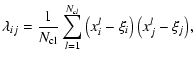
In the present study we use the classical mass ellipsoid
(see e.g. Korn & Korn 1961):
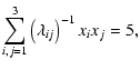 |
(1) |
 |
(2) |
 is the
total number of groups, and
is the
total number of groups, and
 determines the Cartesian coordinates
of the centre of mass of the system.
determines the Cartesian coordinates
of the centre of mass of the system.
The formula determines a 3-dimensional ellipsoidal surface with the
distance from the centre of the ellipsoid equal to the rms deviation
of individual objects in the corresponding direction. This method can
be applied for superclusters with  .
The problems related to the
stability of the method and the influence of observational errors have
been discussed in Jaaniste et al. (1998).
.
The problems related to the
stability of the method and the influence of observational errors have
been discussed in Jaaniste et al. (1998).
In the case of contemporary deep surveys as the LCRS, where the galaxies with measured redshifts cover only a narrow slice, the shape of the ellipsoid strongly depends on the parameters of the survey. For a thin layer it is possible to use a 2D approximation, ignoring the third coordinate (in our case, the declination). Since the geometry of slices is far from a plane-parallel sheet we shall use the 3D algorithm to approximate the shapes of systems. In this way we get 3D objects that correspond to the 3D "slices'' cut from the larger 3D superclusters (Abell superclusters).
In Table 1 we present some parameters of the ellipsoid of concentration for all systems composed of at least 6 LCLGs. In Fig. 2 we plot the distribution of angles between the line-of-sight and the large semiaxes of the LCLG superclusters (Table 1). The diagonal corresponds to a uniform distribution. The systems are moderately elongated (the mean axes ratio 3:1) and show a tendency to be oriented perpendicularly to the line of sight. The same tendency has been found for Abell superclusters (Jaaniste et al. 1998).
![\begin{figure}
\par\includegraphics[width=7.1cm,clip]{H4267F2.ps}\end{figure}](/articles/aa/full/2003/27/aah4267/img37.gif) |
Figure 2: The angle between the line-of-sight and the large semiaxes of the LCLG superclusters (Table 1). The diagonal corresponds to the uniform distribution. |
| Open with DEXTER | |
Here we describe shortly the most prominent Abell superclusters crossed by the LCRS slices.
The most prominent Abell supercluster
crossed by the Northern LCRS slices is the supercluster SCL126 in the
direction of the Virgo constellation (Fig. 3).
Four Abell clusters of total seven member clusters of this supercluster
are located in the Las Campanas slice
within a
sphere of a diameter of about 10 h-1 Mpc. Three of these four
clusters are strong X-ray sources. The fifth X-ray cluster in this
supercluster is Abell 1750, but it is located outside the slice.
This cluster is a merging binary cluster (Donelly et al. 2001).
Four Abell clusters in this supercluster are radio sources. Such a
concentration of rich optical, X-ray, and radio clusters in one
supercluster in a very small volume makes SCL126 one of the most
unusual superclusters currently known.
There are three LCLGs in the central area of the supercluster. All
these groups are unusually rich.
Table 1 shows that the local density in the area of this
supercluster is the largest in the whole survey,
 .
.
![\begin{figure}
\par\includegraphics[width=8.8cm,clip]{H4267F3.ps}\end{figure}](/articles/aa/full/2003/27/aah4267/img39.gif) |
Figure 3: The distribution of Abell clusters (open circles), Las Campanas Loose Groups (triangles) and LCRS galaxies (stars) in the region of the supercluster SCL126 along line-of-sight, with shape ellipses. Open circles denote Abell clusters, triangles - LCLGs, stars - LCRS galaxies. |
| Open with DEXTER | |
Another rich supercluster in this slice is the supercluster SCL100
with 9 member Abell clusters (the supercluster Leo A). The members of this
supercluster are very close to the LCRS slices being located almost
all in one plane. Three member clusters lie in the slice
,
and one in the slice
.
Altogether
there are 26 loose groups from the LCRS in this supercluster. However,
the properties of this supercluster differ from those of SCL126.
There are no X-ray clusters among these clusters. One cluster,
Abell 1200, is a radio source. The distances between the Abell clusters in
this supercluster are quite large, and this supercluster resembles
rather a filament of clusters. Table 1 shows
that this filament-like supercluster is located almost along the
line-of-sight.
![\begin{figure}
\par\includegraphics[width=7.8cm,clip]{H4267F4a.ps}\par\vspace*{2mm}
\includegraphics[width=7.8cm,clip]{H4267F4b.ps}\end{figure}](/articles/aa/full/2003/27/aah4267/img40.gif) |
Figure 4:
The distribution of Abell clusters and Las Campanas loose
groups in the region of the supercluster SCL48 (the
Horologium-Reticulum supercluster) in supergalactic YX (upper panel)
and YZ (lower panel) coordinates in Mpc. Filled circles denote Abell
clusters, open circles - LCLGs from the slice
,
crosses - LCLGs from the slice
,
and  's - LCLGs
from the slice
.
The Abell numbers of the richest
Abell clusters in this supercluster are given (see text). 's - LCLGs
from the slice
.
The Abell numbers of the richest
Abell clusters in this supercluster are given (see text). |
| Open with DEXTER | |
A part of the Sextans supercluster (SCL 88) is seen in all three
Northern slices. The Abell cluster members of the Sextans supercluster
closest to the LCRS slices are A978 (the slice
), and
A970 (the slice
,
this is an X-ray cluster). In the slice
23 groups form a system that is an extension of
this supercluster. The groups themselves in this extension are relatively
poor - the richest loose group here has
 ,
being
poorer than Abell clusters of richness class R = 0.
,
being
poorer than Abell clusters of richness class R = 0.
Another supercluster, seen in the slice
,
is the
supercluster SCL119. Its member cluster Abell 1606 is an X-ray
source and is associated with three loose groups.
The most prominent supercluster crossed by all Southern LCRS slices
(and one of the richest superclusters known) is the Horologium-Reticulum supercluster (SCL48), 47 LCLGs being associated with this
supercluster (Fig. 4). This supercluster contains two
X-ray clusters and a number of APM clusters (Einasto et al.
2002b). One concentration of Abell clusters and LCLGs in this
supercluster is centred on the very rich Abell cluster A3135
(the richness class R = 2, the slice
)
that is
associated with 7 loose groups. Another concentration of clusters in the
Horologium-Reticulum supercluster is crossed by the slice
.
The richest Abell cluster in this region is Abell 3112,
an X-ray and radio source. However, the richest concentration
of LCLGs in this slice is located around another member cluster of this
supercluster, Abell 3133 (the richness class R = 0). A third concentration
of groups and clusters in this supercluster is located around the Abell
cluster 3128 (Rose et al. 2002) at the distance of about
40 h-1 Mpc from the cluster Abell 3135. This concentration,
however, lies outside the boundaries of the LCRS slices. All these
concentrations are connected by filaments of galaxies, groups and
clusters that surround underdense regions (see also Rose et al. 2002).
Another very rich supercluster crossed by the LCRS slices is the
Sculptor supercluster (SCL9). There are five Abell clusters in the
region of the LCRS slices from this supercluster, 4 in the slice
and 1 in the slice
.
Altogether there
are 16 loose groups near these rich clusters in this supercluster.
The supercluster SCL23 in the slice
consists of
two Abell clusters, Abell 2860 (a radio source) and Abell 2911. There are 11 LCLGs in this region. This supercluster is seen in
the ESP survey as a very strong density enhancement in the galaxy
distribution (Vettolani et al. 1997). This supercluster
separates two voids, each of which have diameters of about 100 h-1 Mpc.
On opposite sides of these voids are the Horologium-Reticulum and the
Sculptor superclusters.
The Southern slices
and
cross the supercluster SCL182. All 6 member Abell clusters
of this supercluster are located in these slices. The cluster A3809 is
an X-ray source.
Table 2: Median and upper quartile (in parentheses) values of LCLG properties.
One system consisting of 8
loose groups is located in the slice
in the void
separating the Abell superclusters SCL 88 (Sextans), 126, and 155.
Another such high-density system of loose groups is located in the
slice
at a distance of about 220 h-1 Mpc. The
closest Abell cluster to this system is Abell 1317, that lies at a
distance of about 15 h-1 Mpc from the richest group in this system,
LCLG-12 092. This supercluster has a "spider-like'' appearance.
In the slice
there is a system of 8 loose groups
located between voids at a distance of about 250 h-1 Mpc. An about 100 h-1 Mpc void separates this system from the Horologium-Reticulum
supercluster. There are some galaxy systems in this void, but no rich
clusters or superclusters. This system resembles the Great Wall,
a rich filament of galaxies and groups of galaxies connecting
superclusters.
The existence of supercluster systems that contain only LCLGs and separate huge voids of diameter of about 100 h-1 Mpc agrees with the earlier findings by Einasto et al. (1997) and Frisch et al. (1995). These earlier studies found that huge voids in the supercluster-void network are of similar size, about 100 h-1 Mpc, but the properties of void walls range from those of poor superclusters to very rich superclusters containing tens of rich (Abell) clusters.
Let us now compare the properties of LCLGs in Abell superclusters with the
properties of LCLGs in rich systems of LCLGs containing no Abell
clusters (LCLG.scl and LCLG.slg, respectively; the sample LCLG.slg
includes also the outer members of SCL88 in the slice
).
Several physical properties have been calculated for each group in the
LCLG catalogue (TUC). These include the observed number of group
member galaxies
 ,
the line-of-sight velocity rms
,
the line-of-sight velocity rms
 ,
the virial mass
,
the virial mass
 ,
the total luminosity
,
the total luminosity
 ,
and the Abell counts
,
and the Abell counts
 .
We refer to TUC for
details of how these properties were estimated.
In Table 2 we
give the values of these properties for loose groups from
different systems, as well as for the total sample of LCLGs.
.
We refer to TUC for
details of how these properties were estimated.
In Table 2 we
give the values of these properties for loose groups from
different systems, as well as for the total sample of LCLGs.
Two measures of a group's richness are its observed number of
galaxies,
,
and its Abell count,
,
calculated taking into account the selection
effects (see TUC). We see that if we use these estimated Abell
counts as a measure of the group richness, loose groups in Abell
superclusters tend to be richer than loose groups in systems without
Abell clusters. Only the two richest groups in the sample of systems
of loose groups, LCRS.slg, have the Abell counts larger than 30 - this
population consists of intrinsically poor loose groups. In contrast,
in the population of loose groups in Abell superclusters the mean
Abell count
 and more than 15% of loose groups have
larger than 30. The richest group in this sample has
the Abell count
and more than 15% of loose groups have
larger than 30. The richest group in this sample has
the Abell count
 ,
equivalent to a richness class R=2cluster.
,
equivalent to a richness class R=2cluster.
Additionally, let us take as an example the Abell supercluster SCL222
that consists of two Abell clusters and is probably completely
embedded within the LCRS slice
.
In this supercluster
alone there are 4 loose groups, and three of them are richer than
 - richer than any group from the
sample of loose groups from systems without Abell clusters. This may
indicate that, although the local density of groups is rather high in
the systems without Abell clusters, all loose groups in these systems
are intrinsically poor. This is a hint that the absence of Abell
clusters in these systems is due to the poorness of individual groups
in these region and not due to possible incompleteness in the Abell
catalogue.
- richer than any group from the
sample of loose groups from systems without Abell clusters. This may
indicate that, although the local density of groups is rather high in
the systems without Abell clusters, all loose groups in these systems
are intrinsically poor. This is a hint that the absence of Abell
clusters in these systems is due to the poorness of individual groups
in these region and not due to possible incompleteness in the Abell
catalogue.
The Kolmogorov-Smirnov test shows that the differences in the distribution of group richnesses between the two samples are statistically significant at the 90% confidence level.
The rms line-of-sight velocity of loose groups,
,
in the Abell superclusters is about 1.2 times larger than
that of loose groups from systems without Abell clusters (LCRS.slg).
There are no loose groups in this population with the rms velocity
larger than
 km s-1. The Kolmogorov-Smirnov
test shows that the differences in the distribution of group rms
velocities between the two group samples are statistically
significant at the 99% confidence level.
km s-1. The Kolmogorov-Smirnov
test shows that the differences in the distribution of group rms
velocities between the two group samples are statistically
significant at the 99% confidence level.
Comparison of virial masses of loose groups,
,
shows
that loose groups in Abell superclusters have masses that are about
1.6 times larger than masses of loose groups in systems without
Abell clusters. The Kolmogorov-Smirnov test shows that the
differences in the distribution of group virial masses between the two
samples are statistically significant at the 75% confidence level.
The total luminosities of groups,
,
show that loose
groups in Abell superclusters are about 1.6 times more luminous
than loose groups in systems without Abell clusters. The
Kolmogorov-Smirnov test shows that the differences in the
distribution of group luminosities between the two samples of groups
are statistically significant at the 95% confidence level.
In order to study how far the environmental enhancement of loose group properties extends, we calculated for loose groups in Abell superclusters the distance to the nearest Abell cluster. In Fig. 5 we plot the rms line-of-sight velocities of loose groups in superclusters against the distance to the nearest Abell cluster in a supercluster. This figure shows a decrease in the velocity dispersions of loose groups with an increase in the distance to the nearest Abell cluster. Enhancement of properties of loose groups extends quite far from Abell clusters, up to about 15 - 20 h-1 Mpc. At distances larger than approximately 20 h-1 Mpc (in our sample these loose groups are distant members of the supercluster SCL 48, the Horologium-Reticulum supercluster), this phenomenon becomes weaker.
The loose groups from an outer population of the supercluster SCL88 in
the slice
lie at distances of about 16 h-1 Mpc from
the nearest Abell cluster in this supercluster (this Abell cluster is
seen in the LCRS slice
).
The nearest Abell cluster to the loose groups in the LCRS.slg1 system
is located at a distance of about 30 h-1 Mpc. Likewise, the nearest
Abell clusters to the loose groups in the LCRS.slg2 and LCRS.slg3
systems are at distances of about 15 h-1 Mpc and about 35 h-1 Mpc,
respectively. Thus, groups not belonging to superclusters or those
groups which are outer members of superclusters do not show
environmentally enhanced properties as do the inner members of
superclusters.
To summarise, these results extend the environmental enhancement of mass, velocity dispersion, and luminosity of loose groups in the vicinity of rich clusters of galaxies found by Einasto et al. (2003a) to the loose groups within Abell superclusters. This effect is absent in systems which contain no rich clusters. We found indications that this effect is also absent in the case of loose groups from outer parts of superclusters.
![\begin{figure}
\par\includegraphics[width=8.1cm,clip]{H4267F5.ps}\end{figure}](/articles/aa/full/2003/27/aah4267/img58.gif) |
Figure 5: The rms line-of-sight velocities of loose groups in Abell superclusters against the distances from the nearest Abell cluster in a supercluster. The open circle represents LCLG-12 163, that is located at an end of a filament centred on an Abell cluster from SCL119. |
| Open with DEXTER | |
The large scale distribution of Abell clusters and superclusters was described in Einasto et al. (1997). In particular, it was shown that 75% of very rich superclusters are located in the so-called Dominant Supercluster Plane (DSP) that crosses the Local Supercluster Plane at almost right angles and consists of chains of superclusters and voids between them. Let us now study the distribution of LCLGs with respect to Abell superclusters and the Dominant Supercluster Plane.
Figure 6 shows the distribution of Abell clusters and
the location of the LCRS slices with respect to the supercluster-void
network. The Las Campanas slices cross several rich superclusters in the
Dominant Supercluster Plane: the Sculptor supercluster
and the Horologium-Reticulum supercluster in the Southern sky, and
the Leo A supercluster in the Northern sky. The Southern slice at
goes almost through the DSP.
Of the Northern slices, the slice
at
is closest to the DSP; the other Northern
slices cross the voids between superclusters. The Northern
slice at
crosses the region most devoid of
galaxies and galaxy systems. This may be one of the reasons why the
number of LCLGs in this slice is much smaller than the number of groups
in other slices.
![\begin{figure}
\par\includegraphics[width=14.8cm,clip]{H4267F6a.ps}\par\includegraphics[width=15.4cm,clip]{H4267F6b.ps}\end{figure}](/articles/aa/full/2003/27/aah4267/img59.gif) |
Figure 6: Upper panel: the Abell clusters in equatorial coordinates. Filled circles show the Abell clusters located in superclusters of richness 8 and more members, open circles mark the Abell clusters in less rich superclusters. Solid lines show the location of the LCRS slices, dashed lines - the location of the Dominant Supercluster Plane. Lower panels show intersections of supercluster ellipsoids with the LCRS slices |
| Open with DEXTER | |
In addition, in Fig. 8 we plot the maximum relative supercluster densities from Table 1 against the distances of superclusters. This figure shows that there is no distance-dependent bias for supercluster densities. This means that the selection effects have been taken into account properly when determining the density field superclusters.
Einasto et al. (2003a) and Heinämäki et al. (2003) discussed several selection effects that could affect the properties of loose groups. We analysed the properties of loose groups in high density regions around rich clusters and showed that selection effects cannot artificially enhance the properties of loose groups in high density regions.
In Einasto et al. (2003a), Einasto et al. (2003b) and Einasto et al. (2003c) we discuss also several other distance-dependent selection effects. Our analysis of properties of groups in a wide range of environments (not just in high density environment of superclusters) shows that groups of lower luminosity tend to be located in lower density environment (as shown earlier by Lindner et al. 1995) at all distances.
The orientation of superclusters with respect to the line-of-sight has an excess of systems oriented perpendicular to the line of sight. In Jaaniste et al. (2003) we found a similar tendency of orientations in the case of superclusters of LCLGs determined using the FoF method and a neighbourhood radius R = 12 h-1 Mpc. In a recent study of the 2dF survey Peacock et al. (2001) found evidence of recessional velocities caused by a systematic infall of galaxies into superclusters. Our results on the orientations of superclusters may be evidence of the same effect.
Moreover, the supercluster SCL126 in the direction of the Virgo constellation can be interpreted as an example of such infall. In this case the ellipsoids calculated using data on Abell clusters, loose groups and individual galaxies were shown above (Fig. 3). In all cases the ellipsoid with the axes ratio about 1:4 is located perpendicularly to the line of sight. Jaaniste et al. (1998) found that this is one of the flattest and thinnest superclusters, being located almost perpendicularly with respect to the line of sight. This may be an evidence of the "squashing effect'' of infalling galaxies into superclusters before turnaround or beginning of the relaxation (Kaiser 1987), accompanied by merging and other processes that cause X-ray and radio radiation from clusters in this supercluster (Sect. 4).
![\begin{figure}
\par\includegraphics[width=8.3cm,clip]{H4267F7.ps}\end{figure}](/articles/aa/full/2003/27/aah4267/img60.gif) |
Figure 7:
Luminosities of LCRS loose groups from superclusters
of Abell clusters (filled circles) and from systems without Abell
clusters (open circles)
(in units of solar luminosity
 )
versus the distances of the groups (in h-1 Mpc). )
versus the distances of the groups (in h-1 Mpc). |
| Open with DEXTER | |
.
In this region the concentration
of Abell and X-ray clusters and Las Campanas
loose groups and galaxies in very high.
Superclusters like SCL126 may be detected
though the Sunyaev-Zeldovich effect in
surveys like the forthcoming Planck mission.
Such a high concentration of clusters has been observed so far only in a very few superclusters. Among them are the Shapley supercluster (Bardelli et al. 2000) and the Aquarius supercluster (Caretta et al. 2002). A very small number of such a high density cores of superclusters is consistent with the results from N-body calculations which show that such high density regions (the cores of superclusters that may have started the collapse) are rare (Gramann & Suhhonenko 2002).
In the case of the Horologium-Reticulum supercluster (SCL48) the LCRS data trace rather well two of the three concentrations of galaxies determined in this supercluster, using data on rich clusters (see also Rose et al. 2002).
![\begin{figure}
\par\includegraphics[width=8.1cm,clip]{H4267F8.ps}\end{figure}](/articles/aa/full/2003/27/aah4267/img61.gif) |
Figure 8: Maximum relative densities in superclusters (Table 1) versus the distance of a supercluster. Filled circles correspond to superclusters of Abell clusters, open circles - to systems without Abell clusters. |
| Open with DEXTER | |
.
However, in contrast to SCL126,
the local density in the region of this supercluster
is not high. With its elongated shape this supercluster
resembles a filament. Such long filament-like superclusters
have also been detected in N-body calculations (Faltenbacher
et al. 2002).
We note that the LCRS slices cross the supercluster-void network at such an angle that the 120 h-1 Mpc scale that characterises the distribution of rich clusters and superclusters (Einasto et al. 1994) is not clearly expressed, and we see a smaller scale (of about 100 h-1 Mpc) as an excess in the correlation function of LCRS (Tucker et al. 1997) instead.
These results are in accordance with those by Einasto et al. (2003b) who used a larger sample of groups and clusters from the Sloan survey to show that groups and clusters in high density environments have higher luminosities than those in low density environments.
Our results describe one aspect of the hierarchy of systems in the Universe, earlier characterised using the sizes of voids determined by different objects (Lindner et al. 1995; Arbabi-Bidgoli & Müller 2002).
Several recent studies of the correlation function of nearby groups of galaxies show that properties of groups of galaxies in high density regions are different from properties of groups on average (Giuricin et al. 2001; Girardi et al. 2000; Merchan et al. 2000). Stronger clustering is an indication that these groups could be located in the high density regions of superclusters (Einasto et al. 1997; Tago et al. 2002).
Additionally, several studies of clusters of galaxies have provided evidence that properties of rich clusters depend on their large scale environment (Einasto et al. 2001; Plionis & Basilakos 2002; Schuecker et al. 2001; Chambers et al. 2002; Novikov et al. 1999) up to a distance of about 20 h-1 Mpc. This distance is close to the so-called "pancake scale'' (Melott & Shandarin 1993), and corresponds to the mean thickness of superclusters (Einasto et al. 1994,1997; Jaaniste et al. 1998). This distance is also close to that up to which the environmental enhancement of loose groups hase been detected in the present study.
Suhhonenko (2002) has demonstrated using different N-body simulations that in simulated superclusters more massive clusters are located in the central regions of superclusters.
Gottlöber et al. (2002) and Faltenbacher et al. (2002) analysed high-resolution simulations of formation of galaxies, groups, and clusters and found a significant enhancement of the mass of haloes in the environment of other haloes. This effect is especially significant at scales below 10 h-1 Mpc. Therefore, environmental enhancement of the halo mass is a direct evidence for the process of the hierarchical formation of galaxy and cluster haloes.
We studied the Las Campanas loose groups in superclusters of Abell clusters. We described the superclusters that are crossed by LCRS slices, and the large-scale distribution of the LCLGs in the supercluster-void network.
Our results show that the orientation of superclusters, as determined by LCLGs, has an excess of systems oriented perpendicularly to the line-of-sight. The Las Campanas loose groups in superclusters are richer and more massive than loose groups in systems that do not belong to superclusters. The data about galaxies, loose groups and rich clusters show that the supercluster SCL126 has a very high density core containing several X-ray clusters. This supercluster is located almost perpendicularly in respect to the line-of-sight. We assume that this may be due to infall of galaxies into the supercluster.
Our study indicates the importance of the role of superclusters as high density environment which affects the properties (formation and evolution) of galaxy systems.
Acknowledgements
We thank Erik Tago and Heinz Andernach for providing us with the compilation of the data on Abell clusters. We thank Enn Saar and Sahar Allam for stimulating discussions. The present study was supported by the Estonian Science Foundation grant 4695 and by the Estonian Research and Development Council grant TO 0060058S98. P.H. was supported by the Finnish Academy of Sciences (grant 46733). D.L.T. was supported by the US Department of Energy under contract No. DE-AC02-76CH03000. This study has made use of the NASA/IPAC Extragalactic Database (NED) which is operated by the Jet Propulsion Laboratory, Caltech, under agreement with the National Aeronautics and Space Association.
The distribution of Las Campanas loose groups and rich clusters of galaxies in Las Campanas Redshift Survey slices. Blue spheres represent loose groups, red spheres - Abell clusters, violet spheres - X-ray clusters. Numbers of superclusters of Abell clusters from Einasto et al. (2001) are also shown.
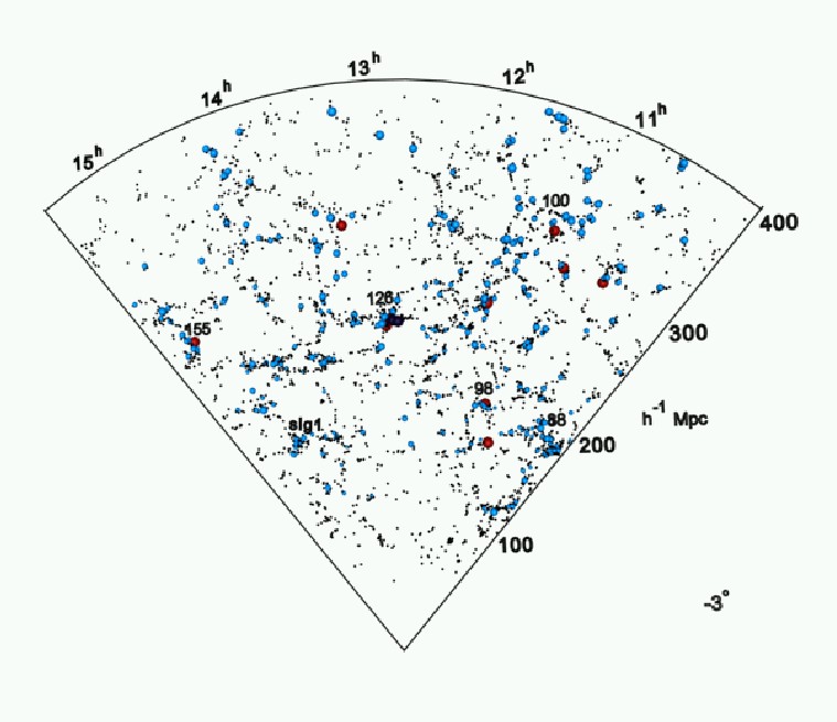 |
Figure 9: The slice delta = -3 degrees |
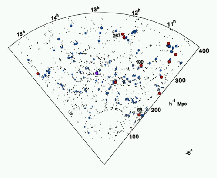 |
Figure 10: The slice delta = -6 degrees |
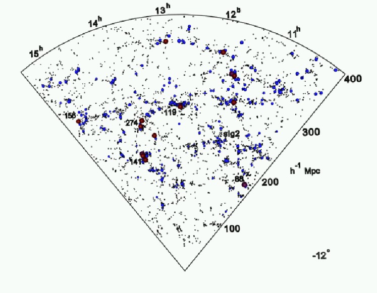 |
Figure 11: The slice delta = -12 degrees |
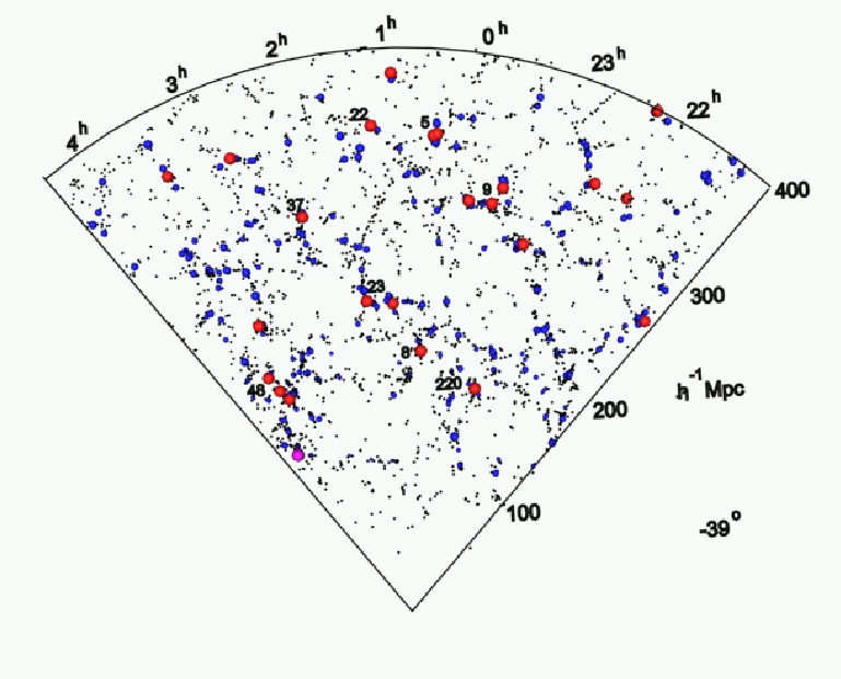 |
Figure 12: The slice delta = -39 degrees |
 |
Figure 13: The slice delta = -42 degrees |
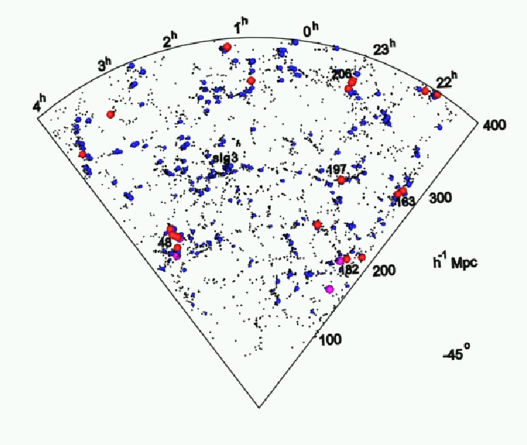 |
Figure 14: The slice delta = -45 degrees |
Animations show the distribution of LCLGs in respect to the supercluster-void network. Here white spheres represent Abell clusters in very rich superclusters and blue spheres represent Las Campanas Loose Groups.
1. Northern sky
2. Southern sky