Contents

• Optimization with numerical simulations of the conjugate altitudes of deformable mirrors in an MCAO system
• 1 Introduction
• 2 MCAO model
• 3 Description of the software employed: CAOS
• 4 Simulation description and simplifications
• 5 Simulation results
• 6 Choosing the DM₂ conjugation altitude
• 7 Conclusions
• References

A&A 404, 1165-1176 (2003)
DOI: 10.1051/0004-6361:20030538

Optimization with numerical simulations of the conjugate altitudes of deformable mirrors in an MCAO system

B. Femenía - N. Devaney

GTC Project, Instituto de Astrofísica de Canarias, Vía Láctea s/n, 38200 La Laguna, Spain

Received 12 February 2003 / Accepted 6 April 2003

Abstract
This article reports on the results of simulations conducted to assess the performance of a modal Multi-Conjugate Adaptive Optics (MCAO) system on a 10 m telescope with one Deformable Mirror (DM) conjugated to the telescope pupil and a second DM conjugated at a certain altitude above the pupil. The main goal of these simulations is to study the dependence of MCAO performance upon the altitude of the high-altitude conjugated DM and thereby determine its optimal conjugation. The performance is also studied with respect to the geometry of the Guide Star constellation when using constellations of Natural Guide Stars (NGS), which are rare, or constellations of Laser Guide Stars (LGS) which would allow large sky coverage.

Key words: intrumentation: adaptive optics - intrumentation: high angular resolution - methods: numerical - atmospheric effects - telescopes

  
1 Introduction

Adaptive Optics (AO) was first proposed by Babcock (1953) as a means to compensate for the loss of spatial resolution of telescopes due to the disturbing effects caused by atmospheric turbulence (Roddier 1981) and thereby obtain diffraction limited resolution. A major limitation of AO is the small size of the Field of View (FoV) over which the correction is effective, referred to as the isoplanatic patch. Under good seeing conditions a typical value for the isoplanatic radius is just a few (2-3) arcsec in the visible ( $0.5~\rm\mu m$) and about 12-18 arcsec in the near infrared ( $2.2~\rm\mu m$). The concept of MCAO as a technique to deliver large corrected FoVs was proposed by Dicke (1975) and later developed by Beckers (1988) with the main goal of increasing the corrected FoV. It did not however receive much attention at that time as the AO community focused on conceptual problems such as obtaining adequate sky coverage with and without the use of Laser Guide Stars (LGS) (Sandler et al. 1994; Le Louarn et al. 1998) and the problems associated with LGS-based AO systems, in particular tip-tilt indetermination and the cone effect. During the early '90s the concept of atmospheric turbulence reconstruction in 3-D (i.e. tomography) was proposed as a solution to overcome the problems associated with sky coverage and the cone effect in LGS-based AO systems (Tallon & Foy 1990). Shortly afterwards, the theoretical foundations of MCAO were developed (see e.g. Johnston & Welsh 1994; Ellerbroek 1994). In the last few years it has been recognised that tomography and MCAO offer the possibility of attaining large corrected FoVs and there is a large on-going effort in MCAO on both the theoretical side (see e.g. Ragazzoni et al. 2000; Rigaut et al. 2000; Fusco et al. 2000,2001; Ragazzoni et al. 1999) and using numerical simulation (see e.g. Ellerbroek 2001; Tokovinin et al. 2001; Flicker et al. 2000; Tordi et al. 2001; Le Louarn 2002; Bello et al. 2001; Ellerbroek & Rigaut 2001; Femenía et al. 2001; Carbillet et al. 2001a; Conan et al. 2001) to assess the performance of MCAO systems.

Conventional AO systems employ a single Deformable Mirror (DM) usually conjugated to the telescope entrance pupil. MCAO requires at least a second DM conjugated to some altitude above the pupil. The addition of a second DM represents a modest increase in complexity (of course the wave-front sensor also has to be modified). Such a dual-conjugate mode is considered as a short term upgrade to the AO system being designed for the 10 m GTC telescope (Devaney et al. 2002) at the Observatorio del Roque de los Muchachos (ORM, Spain). In this work we present numerical simulations of a dual-mirror modal MCAO system for the case of a 10-m telescope. The main goal of our simulations is to determine the optimal conjugation altitude of the high-altitude DM (from now on referred to as DM₂) assuming that the low-altitude DM (DM₁) is conjugated to ground level. Our numerical simulations investigate the dependence of the optimal high-altitude conjugation altitude on the nature of the GS constellation (either NGS or NGS plus LGS constellations are considered), the geometry and the number of reference sources in the GS constellation. These simulation results will be compared with theoretical predictions based on the estimates of Tokovinin & Viard (2001) for the optimal conjugation altitude of DM₂.

2 MCAO model

  
2.1 Modal tomography approach

In modal tomography (Lawrence & Chow 1984; Ragazzoni et al. 1999) one seeks to estimate the coefficients of Zernike expansions of the wavefronts over metapupils defined at the conjugate altitudes of the DMs. The metapupils are circles enclosing the footprints of the beams from the guide stars. If $\overrightarrow{b}_{\rm (g)}$ denotes the Zernike polynomial decomposition of the incoming wavefront when looking at guide star g in the direction $\overrightarrow{\theta }_{\rm (g)}$ (i.e. $W(\overrightarrow{x};~ \overrightarrow{\theta }_{\rm (g)})~ =\sum_{i} ~ b_{i,{\rm (g)}}Z_{i}(\overrightarrow{x}/R)$, with R the pupil radius) then the Zernike polynomial decomposition of the wavefront defined on each of the metapupils to be reconstructed at heights h_l ( $l=1\ldots L$) is $\left\{ \overrightarrow{a}^{(l)}\right\} _{l=1\ldots L}$ which is related to $\left\{ \overrightarrow{b}_{(g)}\right\} _{g=1\ldots G}$ by:

$$\overrightarrow{b}^{\rm T}={\bf P}~ \overrightarrow{a}^{\rm T},$$ (1)

where the subscript $^{\rm ''T''}$ denotes transpose and the different terms in Eq. (1) are:

$$\overrightarrow{b} = \left[\begin{array}{cccc} \overrightarrow{b}... ...{b}_{\rm (G)}\left(\overrightarrow{\theta }_{\rm (G)}\right)\end{array}\right],$$ (2)

 

$${\bf P} = \left[ \begin{array}{cccc} {\bf P}(\overrightarrow{\the... ...cdots {\bf P}(\overrightarrow{\theta }_{\rm (G)};h_{\rm L}) \end{array}\right],$$ (3)

$$\overrightarrow{a} = \left[\begin{array}{cccc} \overrightarrow{a}^{(1)} \overrightarrow{a}^{(2)} \ldots \overrightarrow{a}^{(L)}\end{array}\right]$$ (4)

and in Eq. (3) each of the ${\bf P}(\overrightarrow{\theta }_{\rm (g)};h_{\rm l})$is a Zernike projection matrix relating the Zernike decomposition coefficients of the wavefront defined on the metapupil ( $\overrightarrow{a}^{\rm (l)}$) and $\overrightarrow{b}_{\rm (g)}^{\rm (l)}\left(\overrightarrow{\theta }_{\rm (g)};h_{\rm l}\right)$are the Zernike decomposition coefficients of the wavefront defined on the intersection of the metapupil and the propagation path at the lth layer when looking toward $\overrightarrow{\theta }_{\rm (g)}$:

$$\overrightarrow{b}_{\rm (g)}^{\rm (l)}\left(\overrightarrow{\... ...w{\theta }_{\rm (g)};h_{\rm l})~ \overrightarrow{a}^{\rm (l)}.$$ (5)

The existence of such ${\bf P}(\overrightarrow{\theta }_{\rm (g)};h_{\rm l})$ matrices is demonstrated in Ragazzoni et al. (1999) and an analytical expression for their computation is provided in Femenía & Brusa (2003) and depends exclusively on the geometry of the problem (i.e. on the metapupil radius, radius of the circular region defined by the intersection of the metapupil and the propagation path and the relative position of the circular region with respect to the metapupil center). The required $\left\{ \overrightarrow{a}^{(l)}\right\} _{l=1\ldots L}$ coefficients may be obtained from Eq. (1) by a proper inversion method (e.g. SVD or least square estimator, optimal reconstructor or maximum-a-priori reconstructor).

  
2.2 Implementation in the simulation

The previous description of modal tomography does not give any indication as to how the Zernike polynomial coefficients  $\overrightarrow{b}$of the GS wavefronts are retrieved from real data. In a real wavefront sensor the data will be wavefront local slope measurements (as in the case of Shack-Hartmann and pyramid wavefront sensors) or wavefront local curvature values (as in the case of the curvature sensor). We require a reconstruction process from real measurements to the metapupil Zernike coefficients $\overrightarrow{a}$ without having to first reconstruct the GS Zernike coefficients $\overrightarrow{b}$. This is achieved by means of the interaction matrix ${\bf M}$of the MCAO system linking wavefront sensor outputs ( $\overrightarrow{s}$) and metapupil Zernike coefficients: $\overrightarrow{s}={\bf M}\overrightarrow{a}$. While the ${\bf P}$ matrix in Sect. 2.1 is obtained from purely geometric considerations, building the interaction matrix ${\bf M}$ requires explicit knowledge of the WFS such as the extended size of the GS spot as seen by the WFS, pixelization effects in the WFS or the fact that the WFS sees only a limited FoV. This leads us to use interaction matrices generated by the simulation in which we sequentially place different Zernike polynomials on each layer and register the local tilts produced on each subaperture of each Shack-Hartmann Sensor (SHS) in our MCAO system. In the simulations using LGSs we consider that there is a global tilt subtraction for the wavefront coming from each LGS.

  
3 Description of the software employed: CAOS

The main software tool used is the IDL-based Code for Adaptive Optics Systems (CAOS, Carbillet et al. 2001b,1999). The main feature of CAOS is its modular structure: each elementary physical process is modeled by a specific set of routines (i.e. a module), e.g. the simulation of atmospheric turbulence or the propagation of the wavefront through turbulent layers. This modular design makes CAOS a very versatile tool as it can be extended by the user with new modules as required. The other main feature of the CAOS software is its graphic user interface, the "Application Builder'' (Fini et al. 2000), which helps to design simulation projects in a very straightforward way even for users with no knowledge of IDL. After the graphical design, the Application Builder automatically generates an IDL code which can be run as the desired simulation. In order to simulate MCAO systems new modules have been developed in addition to the modules in the standard CAOS library. A dedicated module conducts the calibration of the MCAO system yielding the interaction matrix: at each layer to be reconstructed we place a single polynomial Z_j at a time and perform the geometrical propagation (i.e. near-field approximation) of the wavefront error corresponding to this Z_j along the line of sight of each Guide Star (GS) down to the SH sensors. The vector of x- and y-slopes from all the SH sensors gives us the column of the matrix associated with the jth Zernike polynomial on the considered layer; this process is then repeated for all the modes to be reconstructed on each layer. The reconstruction process is done with a dedicated module which uses a Least Square Estimator (LSE) and by inverting with Singular Value Decomposition (SVD) the linear relation $\overrightarrow{s}={\bf M}\overrightarrow{a}$between the measured slopes ( $\overrightarrow{s}$) and the coefficients ( $\overrightarrow{a}$) on each reconstructed metapupil. The multi-mirror reconstructor is simulated assuming perfect Zernike DMs in the sense that any mirror is able to generate a pure Zernike mode up to a given mode j and allows different degrees of correction to be used at different layers.

  
4 Simulation description and simplifications

4.1 Generation of Guide Stars (GS)

NGS are simulated as point-like sources at an infinite distance from the telescope and sampling a cylindrical turbulence volume. LGS are simulated as extended sources at a finite distance so that they sample a cone shaped turbulence volume. The width of the LGS is evaluated taking into account the broadening due to diffraction by a launching telescope of 0.5 m diameter, the upward propagation of the laser beam, the perspective elongation of the LGS beacon as seen from the observing telescope and the geometry of the beacon size averaged over the range gate (for Rayleigh LGS) or width of the Na-layer (for Na LGS) using the expression presented in Ellerbroek & Rigaut (2001):

$$\theta _{\rm B}^{2}=\left(\frac{\lambda }{d_{\rm T}}\right)^{... ...2}+\left(\frac{d_{\rm T}~ \delta h}{2\sqrt{3}h^{2}}\right)^{2}$$ (6)

where $\lambda$ is the wavelength of observation ( $\lambda =589.3\ {\rm nm}$for Na LGS, for Rayleigh LGS we consider $\lambda =355\ {\rm nm}$), $d_{\rm T}$the launching telescope diameter, r₀ the Fried parameter at the WFS operation wavelength, L the distance between the launching telescope and the SHS subaperture, h the altitude of the LGS and $\delta h$ the "range gate''. By "range gate'' we mean the vertical distance of the LGS on which we integrate while it is propagating upward. Such a value can be fixed by us when considering Rayleigh LGS (by means of e.g. a Pockels cell). In the case of a Na LGS it is not possible to fix a range gate since the sodium layer drifts in altitude and thus in the above expression we must use the full width of the sodium layer weighted by the fact that the sodium layer has a Gaussian density profile so that an appropriate value in the above expression is $\delta h=5$ km. Then the LGSs are projected onto the WFS so that they look like circular Gaussian spots of width equal to $\theta_{\rm B}$. This neglects the differential elongation due to the finite distance from the telescope to the LGS but on the other hand such an approach is pessimistic since the LGS is not circular but elongated and in practice this involves a loss of resolution only along the elongation direction.

  
4.2 Generation of atmospheric turbulence

For the purpose of our simulations we have constructed a 7-layer profile summarized in Table 1. This profile was built using the measurements of balloon flights (Vernin & Muñoz-Tuñón 1994) launched from the Observatorio del Roque de los Muchachos (ORM). Data from the 6 available balloon flights were used to determine an averaged profile in the following way; first all profiles from the balloon measurements were normalized to have the same total r₀ as the annual mean (i.e.  $r_{0}(500~\mu {\rm m})=0.15~ {\rm m}$) at ORM and then a continuous average profile was generated. Then, following Ellerbroek et al. (1994), a 7-layer turbulence profile was obtained by performing a discrete fit to the continuous average profile that matches the first 14 moments of the continuous turbulence profile.

 

 

Table 1: The ORM average balloon 7-layer profile.

Height $^{{\rm a}}$	Cn,i2	Cn,i2	$r_{0}(0.5~\mu \textrm{m})$	$r_{0}(2.2~\mu \textrm{m})$
(m)	(m1/3 )	(%)	(m)	(m)
4.5	$8.08\times 10^{-14}$	23.0	0.363	2.15
463	$1.04\times 10^{-13}$	29.6	0.312	1.85
1483	$8.64\times 10^{-14}$	24.6	0.348	2.06
4840	$3.86\times 10^{-14}$	11.0	0.565	3.34
11122	$2.25\times 10^{-14}$	6.4	0.781	4.62
14906	$1.76\times 10^{-14}$	5.0	0.905	5.36
18635	$1.40\times 10^{-15}$	0.4	4.13	24.4

$^{{\rm a}}$ Height refers to altitude above the telescope.

Atmospheric turbulent phase screen generation was performed by summing a finite set of Zernike polynomials weighted by a set of coefficients drawn from a Gaussian multivariate distribution of zero mean and covariance matrix as given in Noll (1976), i.e. assuming the turbulence follows Kolmogorov statistics. The truncation of the infinite series implies missing high spatial frequency components. This is easily obviated by truncating at a large enough mode  $j_{{\rm max}}$. The total Strehl ratio due to all missing modes on all layers is estimated to amount to about 10% and this reduction is applied to the iso-Strehl maps. A marginal effect is due to the actual statistics followed by the Zernike coefficients on portions of the phase screens the same size as the telescope pupil. This problem can also be circumvented by the use of a large enough number of Zernike modes when generating the turbulence phase screens.

  
4.3 Propagation through turbulence and wavefront sensing

Propagation of light through atmospheric turbulence is performed by adding linearly the phase fluctuation produced by each turbulent layer which assumes the near-field approximation (Roddier 1981) and corresponds to neglecting diffraction effects in the propagation of the phase of the complex field between layers and from layers to the ground (a similar approximation is implicit when assuming thin layers in Sect. 4.2: diffraction effects between the top and the bottom of the layer are neglected). Ellerbroek (2001) presents results using a code implementing wave-optics for phase propagation and makes a comparison of the results obtained under the near-field approximation for the case of an MCAO system at the Gemini telescope. He concludes that including Fresnel-diffraction in the propagation of light involves a phase rms of only a few nm (<20 nm) with respect to the results obtained with the geometric propagation. Another effect related to not including Fresnel diffraction is that we neglect the effect of scintillation on wavefront sensing. CAOS implements a wave-optics code to simulate the WFS. However the problems of scintillation are not handled since they do not appear in the near-field approximation. Our simulations assume Shack-Hartmann WFS for which the performance dependence on the scintillation has been studied in Voitsekhovich et al. (2001) in the case of open-loop measurements. A direct extrapolation of the results of Voitsekhovich et al. (2001) indicates that for our case with $r_{0}(500~ {\rm nm})=0.15$ m scintillation effects in the WFS will involve errors <8% in the estimation of the high order reconstructed modes. A much more important simplification is that of no noise in the WFS procedure as we are not concerned at this stage with problems associated with sky coverage and by not considering noise we are in the limit of very bright objects.

  
4.4 Least Square Estimator (LSE) reconstructor

Several works (Brusa et al. 2000; Flicker et al. 2000; Fusco et al. 1999,2001; Conan et al. 2001) have focused on estimators for MCAO which assume a real-time knowledge of the statistics of phase perturbations and the turbulence vertical distribution to derive optimal reconstructors operating in open-loop: the so-called Maximum a posteriori (MAP) estimators. In conditions of low Signal-to-Noise Ratio (SNR) it has been shown (Flicker et al. 2000; Le Louarn 2002; Conan et al. 2001) that these optimal reconstructors perform better than the SVD-based reconstruction while yielding similar results in the case of high SNR values. Since we work in the limit of very bright objects (see Sect. 4.3) nothing justifies using MAP estimators here except for the advantage of including knowledge of the vertical distribution of turbulence. On the other hand, it is clear that a MCAO system will be operated in closed-loop which imposes no problem for the implementation of the LSE reconstructor while, to our knowledge, statistics of the residual signal on the WFS have not been derived analytically to be implemented in the design of the MAP reconstructor.

  
4.5 Perfect Zernike deformable mirrors

The DMs considered in these simulations are assumed to be able to reproduce exactly the Zernike modes being reconstructed, that is, if the command is that of generating  a_jZ_j (with ${j=2,\ldots ,153}$) on DM₁ then this is exactly what we get (idem with DM₂but ${j=2,\ldots ,91}$) . This assumption neglects the influence functions of real DMs which in addition to the commanded Z_j mode will probably introduce other modes at a much lower level. Realistic influence functions will be considered in future work using more detailed numerical simulations.

  
4.6 Open-loop operation

Our simulation assumes open-loop operation. In doing this we can easily perform a statistical analysis by generating independent input turbulent wavefronts and retrieving the response of the MCAO system. Open-loop operation neglects degradation of the MCAO system performance due to time-delay errors while on the other hand it gives an underestimation of the performance of the system as compared to closed-loop operation since the WFS is more affected by problems due to the restricted FoV in the SHS and the extended size of the GS.

  
5 Simulation results

In the case of single-conjugate AO with moderate-good correction, the performance may be characterised adequately by a single parameter, namely the on-axis Strehl ratio. The Strehl ratio can be maximised by choosing a threshold value in the SVD reconstruction; singular values lower that the threshold are set to zero and this eliminates modes to which the system is insensitive. In the case of an MCAO system, the performance to be determined is the Strehl ratio over the field of view. We find in our simulations that the Strehl ratio maps are sensitive to the SVD threshold (for example, see Fig. 2). Since the SVD threshold cannot be selected a priori we need criteria for selecting the optimal threshold values for each configuration. 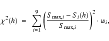In order to characterize SR maps, we extract two parameters which quantify the average Strehl ratio over the field and the amount of variation of the Strehl ratio over the field. For a given Strehl map we determine the value of the Strehl ratio averaged on concentric annular radii (the first annulus is the inner circle of radius  $7\hbox{$^{\prime\prime}$ }$and concentric annuli have an outer radius  $2.5\hbox{$^{\prime\prime}$ }$ larger than the inner radius) and the root mean square deviation of Strehl in each annulus with respect to the averaged Strehl ratio on the circle of radius equal to the annulus outer radius. As shown in the example in Fig. 1 we obtain two families of curves: the first set of curves shows for each SVD threshold value the evolution of Strehl averaged on annuli as a function of the annulus outer radius while the second family of curves shows the evolution of Strehl rms. This process is conducted on contour plots such as those depicted in Fig. 2. To produce these contour plots we interpolate the reconstructed FoV sampled at $15\times 15$locations in the simulation to a finer grid. Due to this interpolation when we get close to the edges we observe a large gradient in S. To avoid a significant bias in the SVD selection process we generate curves of averaged Strehl ratio and Strehl rms on concentric annuli up to a maximum outer radius of about 85% of the whole reconstructed FoV radius. Once we have generated the above sets of curves for each GS configuration and DM₂ conjugation altitude the SVD threshold value selection is based on (i) having flat curves of averaged Strehl within concentric annuli (in general we observe curves which are mostly monotonically increasing or decreasing, so that we select those curves with the lowest peak-to-valley values and/or the lowest gradient on annulus averaged Strehl), (ii) having the smallest Strehl rmsand (iii) in those situations where several threshold values yield similar results based on the previous two points we select the largest SVD threshold value. This is justified in terms of SNR considerations.

  
5.1 Performance using Natural Guide Stars

Figure 1: Example of SVD threshold selection for the case of 3NGS on a circumference of $45\hbox {$^{\prime \prime }$ }$ with DM2 conjugated to 4.7 km. The normalized S rms curve corresponding to $thr_{2}=1.5\times 10^{-4}$ is slightly displaced upward so as not to be superimposed on the curve corresponding to $thr_{3}=2.8\times 10^{-4}$. Here we selected the thr3 curve as the one with the best compromise between the highest S ratio value and the lowest S rms.

Figure 2 shows K-band Strehl maps for the case of having three natural guide stars evenly spaced on a circumference of radius  $30\hbox {$^{\prime \prime }$ }$ in order to reconstruct a circular field of view of  $1\hbox {$^\prime $ }$diameter for several SVD threshold values. The panels correspond to setting different singular value thresholds; it can be seen that the performance is fairly constant until a large number (15) of SVD modes are rejected, some of them with important contributions of absolute Zernike tilts on each of the two reconstructed layers. When only a few SVD modes are rejected (i.e. from $THR=7\times 10^{-5}$ to $THR=3\times 10^{-4}$ involving 2 to 7 SVD modes rejected) the Strehl ratio peaks at the positions of the guide stars as would be expected considering the least-squares reconstruction process employed while the Strehl ratio across the reconstructed FoV is relatively uniform when rejecting 8 to 10 SVD modes ( $THR=4\times 10^{-4}$ to THR=10^-3). This is a general behavior observed in our simulations: uniformity of the Strehl ratio across the reconstructed FoV is achieved at the cost of lowering the peak Strehl ratio at the GS positions by an adequate SVD filtering. Figure 3 shows the best SVD Strehl maps when the three natural guide stars are on a circumference of radius of  $45\hbox {$^{\prime \prime }$ }$, corresponding to a reconstructed FoV of  $1.5\hbox {$^\prime $ }$ diameter, and DM₂ conjugated to 6.1 and 10 km above the telescope pupil. We observe that with DM₂ conjugated to 10 km the average Strehl ratio is significantly smaller than when DM₂ is conjugated to 6.1 km while the variation of the Strehl ratio across the field is more pronounced for DM₂ conjugated to 10 km. Making measurements on the maps it is found that the average Strehl ratio drops from 0.43 to 0.20 and the normalised Strehl rms increases from 16% to 48% (see also Fig. 4). The Strehl rms value when DM₂ is conjugated to 10 km (and to 13 km) is due to such a strong center-to-edge Strehl variation that there is little sense in talking of an average reconstructed Strehl ratio for this scenario.

By varying the DM₂ conjugation altitude in our simulations we obtained that for constellations of 3 NGS the optimal conjugation altitudes are approximately 8.5 km and 6 km for reconstructed FoVs of  $1\hbox {$^\prime $ }$ diameter and  $1.5\hbox {$^\prime $ }$ diameter, respectively. These optimal altitudes are surprisingly low when we consider the vertical distribution of turbulence in the 7-layer model in Table 1. We would expect the pupil-conjugate DM to correct the turbulence in the four lower layers (up to 5 km), and the second DM would therefore be positioned to correct the turbulence in the three upper layers (10-18 km). Tokovinin & Viard (2001) published expressions allowing optimal conjugation altitudes to be calculated for up to three mirrors for a given turbulence profile. Applying these expressions to our case (i.e. two DMs, balloon 7-layer model), we obtain an optimal DM₂altitude of 13 km. We believe the reason for such a disagreement has to do with the strong assumptions in the aforesaid theoretical work: the authors assume that whatever the altitudes of conjugation for the DMs, tomography is able to perfectly reconstruct the wavefront at those altitudes so that the only effect considered is the correction of a continuous turbulence profile by a finite number of DMs. In fact, the further from the telescope we conjugate DM₂, the less overlap between the GS footprints at the metapupil at the DM₂conjugation altitude. This effect will tend to push down the optimal conjugation altitude for DM₂. This statement is supported by the observation that the optimal conjugation altitude is lower for the case of a FoV of  $1.5\hbox {$^\prime $ }$ than for the case of a FoV of  $1\hbox {$^\prime $ }$. In order to further test this hypothesis, we carried out simulations using five natural guide stars and keeping the rest of the parameters of the simulation as in the case of 3 NGS. Increasing the number of NGS in our constellation from 3 to 5 has the effect of increasing the overlap between their footprints and thus we decrease the importance of voids in the metapupil for the wavefront reconstruction at that range. A comparison between the results achieved with constellations of 3 NGS and constellations of 5 NGS is given in the left top and left bottom panels in Fig. 4 where we plot the average Strehl ratio on the reconstructed FoV as a function of the DM₂ conjugation altitude and the Strehl ratio rmsvariation, respectively (the right top and right bottom panels of Fig. 4 show the results obtained when considering different LGS constellations plus an on-axis NGS and which will be the subject of the following sections). We can see in Fig. 4 that when increasing the number of NGSs from 3 to 5 NGS the conjugation altitude of DM₂also increases and this effect can only be due to a better sampling (and reconstruction) of the turbulence at the height at which DM₂is conjugated. From these results we conclude that the effect neglected by Tokovinin & Viard (2001) is very important when determining the best DM₂ conjugation altitude.

Figure 2: Strehl maps for several SVD threshold values in a reconstructed FoV of  $1\hbox {$^\prime $ }$ diameter with DM2 conjugated to 8.4 km and 3NGS on a circumference of  $30\hbox {$^{\prime \prime }$ }$ radius.

Figure 3: Strehl maps for a reconstructed $1.5\hbox {$^\prime $ }$ FoV for DM2 conjugated to 6.1 km and 10. km for a constellation of 3NGS on a circumference of  $45\hbox {$^{\prime \prime }$ }$ radius. These maps correspond to the best SVD case for each DM2 conjugation altitude.

Figure 4: Summary of simulation results. Top panels show the dependence of the MCAO average Strehl ratio on the conjugation altitude of DM2. The bottom panels give the normalized rms of the averaged Strehl ratio on the 83% radius annulus (see main text in Sect. 5 for further details).

Figure 5: Checking two constellation geometries employing 5 NGS. On the left panel the Strehl map when the 5NGS are evenly arranged on the vertices of a regular pentagon within a $1.5\hbox {$^\prime $ }$ FoV. On the right panel the results when 4 NGSs are placed on the vertices of a square and 1 NGS is placed on the FoV center. Both panels correspond to having DM2 conjugated to 10 km above the telescope pupil.

Figure 6: Left panel shows the best SVD Strehl map in a reconstructed FoV of  $1\hbox {$^\prime $ }$ diameter with DM2 conjugated to 10 km and 4 LGS on a circumference of $41.46\hbox {$^{\prime \prime }$ }$ radius plus one on-axis bright NGS (i.e. wave-front sensing on the on-axis NGS is up to the same order as with any LGS). Right panel is the Strehl map corresponding to the reconstruction of a  $1.5\hbox {$^\prime $ }$ diameter FoV with DM2 conjugated to 10 km and 5 LGS on a circumference of  $56.46\hbox {$^{\prime \prime }$ }$ radius plus one on-axis bright NGS.

We also compared two different geometries employing 5 NGS: placing all NGS on the vertices of a pentagon or putting 4 of them on the corners of a square and one at the center. It turns out that it is the latter configuration which yields better results (see top left panel in Fig. 4 and iso-Strehl contour plots in Fig. 5) despite the fact that it leaves unsampled a slightly bigger portion of the metapupil. This suggests that not only the fractional sampling of the metapupil is important but also the distance of points within the reconstructed FoV to the GS. Although we have not conducted any test to check our explanation of this effect we believe that this may be due to the LSE reconstruction in which by definition the best reconstructed positions are those corresponding to the GS positions while for a MAP reconstructor we may encounter a different behavior since it is built by optimizing the reconstruction at a set of positions which do not have to be coincident with those of the GS.

  
5.2 Performance using Sodium Laser Guide Stars

The probability of finding constellations of 3 (not to mention 5) bright natural guide stars arranged to nicely span fields of $1{-} 1.5~ \hbox{$^\prime$ }$ is very low. As an indication, using the Guide Star Catalogue-II we estimate that the probability of finding three stars brighter than $m_{\rm R}=16$, which is an optimistic value for limiting guide star magnitude, is approximately 3% for a field of  $2\hbox{$^\prime$ }$ at galactic coordinates $(l,b)~ =~ (90\hbox{$^\circ$ },40\hbox{$^\circ$ } )$, and this value will be further reduced when requiring the 3 NGS to be properly arranged. In view of these considerations it will be necessary to employ laser guide stars (LGS) in order to provide reasonable sky coverage for star-oriented MCAO systems, at least on 8-10 m telescopes.

It has already been pointed out by different authors (see e.g. Ellerbroek & Rigaut 2001) that the indetermination of the tip-tilt of individual LGS leads to tip-tilt anisoplanatism in an LGS-based MCAO system. The tip-tilt anisoplanatism may be solved in a natural way by detecting the tip-tilt of several NGS in the FoV (Rigaut et al. 2000). In the Gemini-South MCAO system it is planned to reconstruct the tip-tilt using three dim (i.e. $m_{\rm R}\sim 19{-}20$) natural guide stars, and the sky coverage in the K band is predicted (Rigaut et al. 2000) to be 15% and 80% at Galactic pole and $b=30\hbox{$^\circ$ }$, respectively. Alternative schemes can be derived by considering that tip-tilt anisoplanatism mainly arises from turbulence-induced quadratic wavefront errors (i.e. defocus and astigmatism) at altitudes which cannot be determined from the multiple-LGS measurements. If quadratic measurements are made simultaneously with guide stars at different ranges, then it may be possible to correct the tip-tilt anisoplanatism. One approach along these lines is to make wavefront measurements on a natural guide star simultaneously with the laser guide stars. We determine the performance of such an approach here for fields of view of diameter  $1\hbox {$^\prime $ }$ and  $1.5\hbox {$^\prime $ }$. In the case of the smaller field of view we employ four Na LGS on a circumference spanning the field of view plus one on-axis NGS. In the case of the  $1.5\hbox {$^\prime $ }$ field of view we consider two Na LGS configurations; (i) four LGS spanning the field of view plus one on-axis NGS (ii) five LGS on a circumference spanning the field of view plus one on-axis NGS. The circumferences on which the LGS are placed are somewhat larger than the fields of view so that the metapupil sizes are the same when using cone shaped beams from the LGS as when using cylindrical-shaped beams from NGS placed at the edge of the field of view. Figure 6 shows the best Strehl maps for the  $1\hbox {$^\prime $ }$ FoV (left panel) and $1.5\hbox {$^\prime $ }$ FoV (right panel), employing constellations of 4 off-axis LGS+ on-axis NGS and 5 off-axis LGS + on-axis NGS, respectively. For the  $1\hbox {$^\prime $ }$ FoV case the average Strehl ratio is similar to that obtained on the same field of view using 3 NGS although it exhibits a larger peak-to-valley value. The rms Strehl variation is similar to the 3 NGS case but it does not rise steeply when DM₂ is conjugate to an altitude higher than the optimal which for the LGS case is approximately 10 km while in the case of NGS constellation it was about 8.5 km. In the case of the $1.5\hbox {$^\prime $ }$ FoV the average Strehl ratio is almost the same for both 4LGS and 5LGS configurations. The optimal altitude occurs in the range 8-10 km. If DM₂ is conjugate to an altitude higher than the optimal then the average Strehl ratio is higher and the rms variation is lower when 5 LGS are employed rather than 4 LGS.

  
5.3 Hybrid Rayleigh-Na system performance

The natural guide star employed to measure quadratic modes has to be bright, thereby again compromising sky coverage. An alternative approach to solving the tip-tilt anisoplanatism caused by the quadratic modes consists of employing both Rayleigh and Na LGS as well as a single natural guide star which is only used to determine global tip-tilt (Femenía 2003; Ellerbroek & Rigaut 2001; Femenía et al. 2001). Here we apply the algorithm described in Femenía (2003) whose starting point is to realize that unresolved second order modes in LGS-based tomography can be reconstructed using an LGS constellation made at several altitudes (e.g. Rayleigh + sodium LGSs, or Rayleigh LGSs at different altitudes) as shown by Brusa et al. (2000). The reconstruction process consists of two stages in which barycenter tip-tilt is measured from a NGS and in parallel we perform tomography with the LGS constellation placed at at least two different altitudes. From the LGS tomography we obtain a reconstruction of all modes starting from the Zernike second-order modes and this information is used together with the NGS barycenter tip-tilt to obtain an estimate of the global Zernike tilts in the entire reconstructed FoV. The hybrid technique may be implemented in different ways, in particular Femenía (2003) considers a single on-axis Rayleigh LGS on which to conduct high-order wave-front sensing while Ellerbroek & Rigaut (2001) consider several off-axis Rayleigh LGS coupled to low-order WFS. Other parameters to be optimized include the height of the Rayleigh LGS and the wavelength for the Rayleigh LGS. Given the number of new parameters to be investigated the results we present here are by no means exhaustive but only preliminary to give an idea of the potential of the technique. We assume two configurations of 4 Na LGS and 5 Na LGS evenly arranged on a circumference of  $56.45\hbox{$^{\prime\prime}$ }$ radius (so that the reconstructed FoV is $1.5\hbox {$^\prime $ }$) plus an on-axis Rayleigh LGS. The Na LGSs are observed at  $589\ {\rm nm}$ and the Rayleigh LGS at $355\ {\rm nm}$ with $16\times 16$subaperture SHSs. The rest of the simulation parameters (atmospheric profile, number of CCD pixels and SHS FoV, no noise in the SHS, number of reconstructed modes, etc.) are the same as in the simulations with NGS and LGS+on-axis NGS. The top panels a) and b) in Fig. 7 shows the reconstruction across the $1.5\hbox {$^\prime $ }$ FoV for the cases of 4 Na LGS and 5 Na LGS, respectively.

Figure 7: Strehl maps for two LGS geometries employing the hybrid LGS constellations. Panel a) corresponds to using 4 Na LGS at 90 km with an off-axis angle of $56.46\hbox {$^{\prime \prime }$ }$ (in order to provide a corrected  $1.5\hbox {$^\prime $ }$ FoV) and an on-axis tip-tilt NGS. Panel b) corresponds to using 5 Na LGS at 90 km with an off-axis angle of  $56.46\hbox {$^{\prime \prime }$ }$ plus an on-axis Rayleigh LGS at 30 km and an on-axis tip-tilt NGS. Both cases consider DM2 conjugated to 10 km. Panels c) and d) are the same as panels a) and b), respectively except that tip-tilt is perfectly removed. This ideal exercise supports our interpretation on the limited level of reconstruction being mainly caused by residual tip-tilt modes.

On comparing the results from the constellation using 4 Na LGS against the results using 5 Na LGS we see a limited gain. This limited performance gain is a consequence of the limited reconstruction along the on-axis direction which in turn is used to reconstruct the Zernike tip-tilt modes across the entire reconstructed FoV. This statement is supported by the levels of reconstruction attained if we assume perfect reconstruction of the Zernike tip-tilt modes across the entire FoV as depicted in panel c) in Fig. 7 for the case of 4 Na LGS at  $56\hbox{$^{\prime\prime}$ }$ and in panel d) in Fig. 7 for the case of 5 Na LGS at  $56\hbox{$^{\prime\prime}$ }$; in both cases also considering on-axis Rayleigh LGS at 30 km and on-axis tip-tilt NGS. When comparing in Fig. 7 the bottom panels (perfect correction of Zernike tip-tilt across the entire FoV) against the top panels (actual correction of Zernike tilts) we verify that in the latter figures there is a small amount of tilt anisoplanatism caused by a worse correction of higher-order modes (especially second-order modes) in the on-axis direction. This in turn translates into tilt anisoplanatism when using those higher-order modes to reconstruct off-axis Zernike tilts. This situation also appeared when dealing with 5 NGS where we observed that the best configuration is that corresponding to 4 NGS on the corners of a square plus one on-axis NGS rather than all 5 NGS on the vertices of a pentagon. Based on this conjecture it would be more effective having 4 Na LGS distributed on the vertices of a square plus one on-axis Na LGS than having all 5 Na LGS distributed on the vertices of a pentagon.

   
6 Choosing the DM₂ conjugation altitude

As seen in Fig. 4 the optimal DM₂conjugation altitude depends very strongly on the GS nature and configuration. In the case of observing 3NGS on the vertices of equilateral triangles on a circumference of radius  $30\hbox {$^{\prime \prime }$ }$ or  $45\hbox {$^{\prime \prime }$ }$ the optimal altitudes are about 8.5 and 6.0 km, respectively. When considering 5 NGSs the optimal DM₂ conjugation altitude is 10 km. When hybrid LGS constellations and a single tip-tilt NGS are used aiming at a reconstructed FoV of $1.5\hbox {$^\prime $ }$ the best DM₂ conjugation altitude occurs in the range [8, 11] km with little variation of performance within that range leaving the final decision to opto-mechanical considerations. In order to find an optimal DM₂ conjugation altitude that best suits all possible GS configurations cases in this work we consider the following figure of merit:

$$\chi ^{2}(h)~ =~ \sum _{i=1}^{9}\left(\frac{S_{{\rm max},i}-S_{i}(h)}{S_{{\rm max},i}}\right)^{2}\cdot w_{i},$$

where h denotes a generic DM₂ conjugation altitude, the index ${i=1,\ldots ,9}$ runs over all the GS configurations in this work, $w_{\rm i}$ weights different GS configurations, $S_{\rm max,i}$is the maximum Strehl ratio achieved with the ith GS configuration and S_i(h) is the achieved Strehl ratio with the ith GS configuration when conjugating DM₂ to altitude h above the telescope entrance pupil.

 

 

Table 2: Different normalized-to-maximum weighting sets used to obtain the DM₂conjugation altitude. Values marked with superindex ^"a''should be further reduced when requiring proper arrangement of the NGSs.

GS Configuration	w1	w2	w3	w4
3 NGS @ $30\hbox {$^{\prime \prime }$ }$	1.00	1.00	$9\times 10^{-4}$ $^{{\rm a}}$	0.03 $^{{\rm a}}$
3 NGS @ $45\hbox {$^{\prime \prime }$ }$	1.00	1.00	$9\times 10^{-3}$ $^{{\rm a}}$	0.1 $^{{\rm a}}$
5 NGS @ $45\hbox {$^{\prime \prime }$ }$	1.00	0.60	$6\times 10^{-5}$ $^{{\rm a}}$	0.008 $^{{\rm a}}$
4 NGS @ $45\hbox {$^{\prime \prime }$ }$ + NGS	1.00	0.60	$6\times 10^{-5}$ $^{{\rm a}}$	0.008 $^{{\rm a}}$
4 LGS @ $41\hbox{$^{\prime\prime}$ }$ + NGS	1.00	0.40	0.22	0.47
4 LGS @ $56\hbox{$^{\prime\prime}$ }$ + NGS	1.00	0.40	0.44	0.67
5 LGS @ $56\hbox{$^{\prime\prime}$ }$ + NGS	1.00	0.30	0.44	0.67
Hybrid: 4 Na LGS	1.00	0.20	1.00	1.00
Hybrid: 5 Na LGS	1.00	0.15	1.00	1.00

As the $\chi ^{2}$ mimization process will depend on $\left\{ w_{i}\right\}$ we have considered the sets of weights listed in Table 2: the first weighting set (i.e. column w₁ in Table 2) gives equal importance to all GS configurations, weighting set $\left\{ w_{2}\right\}$is focused on avoiding system complexity and thus assigns higher weight to simpler systems while weighting sets $\left\{ w_{3}\right\}$and $\left\{ w_{4}\right\}$ are derived from simple sky coverage considerations based on star counts from the Guide Star Catalogue-2 at $(l,b)~ =~ (90\hbox{$^\circ$ },40\hbox{$^\circ$ } )$ and assuming that for the NGS we require at least $m_{\rm R}\lesssim 16$ when it is used for high-order mode reconstruction and $m_{\rm R}\lesssim 18.5$ when it is only used for tip-tilt reconstruction (i.e. as in the case of the hybrid laser configurations). The difference between weighting sets $\left\{ w_{3}\right\}$and $\left\{ w_{4}\right\}$ is that the former is proportional to the probability of finding the required number of NGSs in the GS configuration and the second is proportional to the square root of that probability (i.e. $w_{4,i}=\sqrt{w_{3,i}}$ where index i runs over the different GS configurations under study). This choice for $\left\{ w_{3}\right\}$ and $\left\{ w_{4}\right\}$ is very qualitative but given the small difference between the results obtained with them (see Table 3) we are confident that a detailed sky coverage analysis is likely to differ little from the results obtained here. The $\chi ^{2}(h)$minimization process yields an "optimal'' DM₂ conjugation altitude as a function of the weighting set. The first and second columns in Table 3 give the DM₂ conjugation altitude for which a given GS configuration attains its maximum Strehl ratio and the Strehl ratio itself. Columns 3 to 6 give Strehl ratios for each GS configuration when the DM₂ is conjugated to the joint optimal conjugation altitude according to the weighing set under consideration (i.e. $S_{\rm opt,1}$ corresponds to using w₁); the value of such optimal conjugation altitude for each weighting set being displayed in parenthesis below each column title. The last two columns in Table 3 give the Strehl ratio and fractional decrease with respect to $S_{\rm max}$, respectively, when DM₂is conjugated to 8 km.

  
7 Conclusions

Modal MCAO in the "classical'' star-oriented fashion holds the promise to reconstruct FoVs as large as  $1.5\hbox {$^\prime $ }$ in diameter. Ideally one would like to rely on NGS constellations but the chances of finding a suitable one is extremely low even for the simplest case of 3NGS. Thus if one wants to build a star-oriented MCAO system which can be used over a significant fraction of the sky one must necessarily consider LGS-based MCAO systems. However, one then has to face the tip-tilt problem and the indetermination of second-order modes. The simplest approach to LGS-based MCAO systems is that of relying on a bright enough NGS on which one could perform not only tip-tilt & second-order sensing but also high-order WFS. This yields poor results and the initially surprising result that performance does not improve significantly when increasing the number of Na LGSs from 4 to 5. In any case, whether we use 4 Na LGS or 5 Na LGS the reconstructed FoV is strongly affected by tip-tilt anisoplanatism and the reconstruction is extremely sensitive to the SVD filtering process which in practice will be determined by the SNR in the WFS measurements. We also remark that such a naive approach also has small sky coverage as it requires a star which is bright enough to obtain high-order wavefront measurements. However, with hybrid LGS constellations (Sect. 5.3) it may be possible to obtain good levels of reconstruction. Taking the sky coverage values obtained with the three tip-tilt NGS scheme considered by Gemini (see Sect. 5.2) and assuming equivalent magnitude requirements for the tip-tilt NGS with hybrid LGS constellations it is expected that this approach can be applied to a larger fraction of the sky as only a single tip-tilt NGS is required. There is a lot of room for possible improvements to the technique used (Femenía 2003).

 

 

Table 3: Finding the optimal DM2 conjugation altitude.

			$S_{\rm opt,1}$	$S_{\rm opt,2}$	$S_{\rm opt,3}$	$S_{\rm opt,4}$	S	$\varepsilon ~ (\%)$
GS Configuration	$h_{\rm max}$	$S_{\rm max}$	(7.7 km)	(6.7 km)	(8.4 km)	(9.0 km)	(8.0 km)
3 NGS @ $30\hbox {$^{\prime \prime }$ }$	8.7	0.61	0.61	0.60	0.61	0.61	0.61	-0.1
3 NGS @ $45\hbox {$^{\prime \prime }$ }$	6.0	0.43	0.37	0.41	0.35	0.30	0.36	-15.5
5 NGS @ $45\hbox {$^{\prime \prime }$ }$	10.8	0.55	0.52	0.51	0.53	0.54	0.53	-4.1
4 NGS @ $45\hbox {$^{\prime \prime }$ }$ + NGS	10.1	0.63	0.62	0.61	0.63	0.63	0.62	-1.8
4 LGS @ $41\hbox{$^{\prime\prime}$ }$ + NGS	11.1	0.57	0.54	0.53	0.55	0.56	0.59	-4.5
4 LGS @ $56\hbox{$^{\prime\prime}$ }$ + NGS	10.2	0.45	0.43	0.41	0.44	0.44	0.43	-3.6
5 LGS @ $56\hbox{$^{\prime\prime}$ }$ + NGS	11.4	0.47	0.43	0.42	0.45	0.45	0.44	-6.0
Hybrid: 4 Na LGS	9.3	0.38	0.37	0.36	0.38	0.38	0.37	-1.8
Hybrid: 5 Na LGS	9.5	0.40	0.39	0.38	0.40	0.40	0.40	-2.2

The optimal DM₂ conjugation altitude depends strongly on the guide star constellation used. When considering NGS constellations our MCAO simulations give results in disagreement with the theoretical work by Tokovinin & Viard (2001) which would place DM₂ at about 13 km above telescope pupil (Devaney et al. 2002). The reason for such disagreement is believed to be caused by the strong assumptions in these theoretical works resulting in overestimating the DM₂conjugation altitude. From our study based on detailed numerical simulations we consider that a suitable DM₂ conjugation altitude for a 10-m class telescope is around 8 km and thus we are considering such an option for the design of the AO system at the GTC telescope which considers an initial AO system with a single corrector but upgradeable to a dual-conjugate system. It has been argued that the aforementioned theoretical works would be applicable to the case of extremely large telescopes (30-100 m diameter) as the main limiting assumption (i.e. full metapupil coverage by overlapping the GS beams at the reconstructed layers) is relaxed and it should be possible to fulfill the requirement of perfect wavefront reconstruction at each metapupil. However, one should consider that the larger the telescope diameter, the larger the number of modes required in order to reach the same Strehl Ratio as with a smaller telescope diameter. It follows from this consideration that with extremely large telescopes, although the metapupil coverage is nearly complete, the importance of small gaps in the metapupil coverage is much more important, this implying that the assumptions in the above theoretical works may not be realistic even for extremely large telescopes.

Our last conclusion regards a rule of thumb indicated by our simulations: given a fixed number of GS (either LGS or NGS) the best MCAO performance occurs for the constellation configuration that minimizes the distance from any point in the FoV to a GS position. As we have seen although 5 GS on the vertices of a pentagon give a larger covered surface of the metapupil than 4 GS on the square vertices plus one on-axis GS, the latter configuration yields the better reconstruction.

We would like to end with a comment on the turbulence profile used in our simulations. It has been derived from only 6 turbulence profiles at the ORM obtained with balloon flights which is a rather small sample of turbulence profiles. A larger set of turbulence profiles would be desirable in order to obtain a more significant average profile at ORM. In any case, all the simulations were also conducted on a modified version of the average profile and the optimal conjugation altitude of DM₂ remained essentially the same.

Acknowledgements

The Guide Star Catalogue-II is a joint project of the Space Telescope Science Institute and the Osservatorio Astronomico di Torino. Space Telescope Science Institute is operated by the Association of Universities for Research in Astronomy, for the National Aeronautics and Space Administration under contract NAS5-26555. The participation of the Osservatorio Astronomico di Torino is supported by the Italian Council for Research in Astronomy. Additional support is provided by European Southern Observatory, Space Telescope European Coordinating Facility, the International GEMINI project and the European Space Agency Astrophysics Division.

References

 
• Babcock, H. W. 1953, PASP, 65, 229 NASA ADS  
• Beckers, J. M. 1988, Proceedings of the ESO Conf. on Very Large Telescopes and their Instrumentation, 693  
• Bello, D., Conan, R., Leroux, B., et al. 2001, in Beyond Conventional Adaptive Optics, ESO Conf. Workshop Proc., 58, 231  
• Brusa, G., Riccardi, A., et al. 2000, Proc. SPIE, 4034, 190  
• Carbillet, M., Femenía, B., Delplancke, F., et al. 1999, Proc. SPIE, 3762, 378  
• Carbillet, M., Femenía, B., Esposito, S., Brusa, G., & Correia, S. 2001a, in Beyond Conventional Adaptive Optics, ESO Conf. Workshop Proc., 58, 259  
• Carbillet, M., Fini, L., Femenía, B., et al. 2001b, in Astronomical Data Analysis Software and Systems X, vol. 10, ASP Conf. Ser., 238, 249  
• Conan, J.-M., Le Roux, B., Bello-Figueroa, C., Fusco, T., & Rousset, G. 2001, in Beyond Conventional Adaptive Optics, ESO Conf. Workshop Proc., 58, 209  
• Devaney, N., Rodríguez Espinosa, J. M., Cardwell, A., Filgueira, J. M., & Femenía, B. 2002, Adaptive Optics for the GTC. Conceptual Design, Tech. Rep. GEN/OPTI/0077-L, GTC Project  
• Dicke, R. H. 1975, ApJ, 198, 605 NASA ADS  
• Ellerbroek, B. 2001, in Beyond Conventional Adaptive Optics, ESO Conf. Workshop Proc., 58, 239  
• Ellerbroek, B. L. 1994, J. Opt. Soc. Am. A, 11, 783 NASA ADS  
• Ellerbroek, B. L., Pompea, S. M., Robertson, D. J., & Mountain, C. M. 1994, in Adaptive Optics in Astronomy, ed. M. A. Ealey, & F. Merkle, Proc. SPIE, 2201, 421  
• Ellerbroek, B. L., & Rigaut, F. 2001, J. Opt. Soc. Am. A, 18, 2539 NASA ADS  
• Femenía, B. 2003, in preparation  
• Femenía, B., & Brusa, G. 2003, in preparation  
• Femenía, B., Carbillet, M., Riccardi, A., Esposito, S., & Brusa, G. 2001, Proc. SPIE, 4494, 132  
• Fini, L., Carbillet, M., & Riccardi, A. 2000, in Astronomical Data Analysis Software and Systems X, ASP Conf. Ser., 238, 253  
• Flicker, R., Rigaut, F., & Ellerbroek, B. 2000, Proc. SPIE, 4007, 1032  
• Fusco, T., Conan, J., Rousset, G., Mugnier, L. M., & Michau, V. 2001, Opt. Soc. Am. J., 18, 2527 NASA ADS  
• Fusco, T., Conan, J.-M., Michau, V., Mugnier, L., & Rousset, G. 1999, Proc. SPIE, 3763  
• Fusco, T., Conan, J.-M., Michau, V., Rousset, G., & Mugnier, L. 2000, Proc. SPIE, 4007, 1044  
• Johnston, D. C., & Welsh, B. M. 1994, J. Opt. Soc. Am. A, 11, 394 NASA ADS  
• Lawrence, G. N. & Chow, W. W. 1984, Opt. Lett., 9, 267 NASA ADS  
• Le Louarn, M. 2002, MNRAS, 334, 865 NASA ADS  
• Le Louarn, M., Foy, R., Hubin, N., & Tallon, M. 1998, MNRAS, 295, 756 NASA ADS  
• Noll, R. J. 1976, J. Opt. Soc. Am. A, 66, 207 NASA ADS  
• Ragazzoni, R., Farinato, J., & Marchetti, E. 2000, Proc. SPIE, 4007, 1076  
• Ragazzoni, R., Marchetti, E., & Rigaut, F. 1999, A&A, 342, L53 NASA ADS  
• Rigaut, F., Ellerbroek, B. L., & Flicker, R. 2000, Proc. SPIE, 4007, 1022  
• Roddier, F. 1981, in Progress in Optics, ed. E. Wolf, vol. 19 (Elsevier), 281  
• Sandler, D. G., Stahl, S., Angel, J. R. P., Lloyd-Hart, M., & McCarthy, D. 1994, J. Opt. Soc. Am. A, 11, 925 NASA ADS  
• Tallon, M., & Foy, R. 1990, A&A, 235, 549 NASA ADS  
• Tokovinin, A., Le Louarn, M., Viard, E., Hubin, N., & Conan, R. 2001, A&A, 378, 710 NASA ADS  
• Tokovinin, A., & Viard, E. 2001, J. Opt. Soc. Am. A, 18, 873 NASA ADS  
• Tordi, M., Ragazzoni R., & Diolati, E. 2001, in Beyond Conventional Adaptive Optics, ESO Conf. Workshop Proc., 58, 223  
• Vernin, J., & Muñoz-Tuñón, C. 1994, A&A, 284, 311 NASA ADS  
• Voitsekhovich, V. V., Orlov, V. G., & Sanchez, L. J. 2001, A&A, 368, 1133 NASA ADS