A&A 403, 1059-1065 (2003)
DOI: 10.1051/0004-6361:20030413
Long-term flux density variations of pulsars:
Theoretical structure functions and comparisons with observations
A. Z. Zhou
1,3 -
X. J. Wu
1,2,3 -
A. Esamdin
2,1,3
1 - Department of Astronomy, Peking University, Beijing
100871, PR China
2 -
the National Astronomical Observatories, the Chinese Academy of
Sciences, Beijing 100012, PR China
3 - CAS-PKU Joint Beijing Astrophysics Center, Beijing
100871, PR China
Received 6 June 2002 / Accepted 6 March 2003
Abstract
By means of the refractive interstellar scintillation theory (RISS),
the flux density structure functions of PSRs B1642-03, B0736-40,
B0740-28 and B0329+54 are calculated and
compared with the observations at 610 MHz by Stinebring et al. (2000,
hereafter S2000). The
theoretical results are in good agreement with observations and
the spectra of the electron density fluctuation are all consistent with the
Kolmogorov spectra. The theoretical modulation indices m are
comparatively less sensitive to the distance H from the observer
to the scattering screen but critically depend on the scattering
strength
 .
The structure function does not
change remarkably with the variation of H if the scattering
screen is closer to the pulsar than to the observer. The results
in this paper indicate that the flux density variations observed
for these four pulsars are due to a propagation effect (refractive
scintillation), not to the intrinsic variability.
.
The structure function does not
change remarkably with the variation of H if the scattering
screen is closer to the pulsar than to the observer. The results
in this paper indicate that the flux density variations observed
for these four pulsars are due to a propagation effect (refractive
scintillation), not to the intrinsic variability.
Key words: stars: pulsars: general - radio continuum: stars - ISM: structure - scattering
The phenomenon of pulsar scintillation was recognized soon after
the discovery of pulsars (Hewish et al. 1968) and this field has
grown significantly since then (Cordes et al. 1986; Gupta et al.
1993, 1994; Armstrong et al. 1995).
Radio waves propagating in the interstellar medium are scattered
by the galactic electrons with random density fluctuations. The
scattering process will enlarge the angular sizes of pulsars and
produce random flux density fluctuations in space and frequency
domains on the observing plane. The spatial variations are mapped
to temporal variations by the relative motion between the pulsar,
scintillation medium and the observer.
In the strong scattering region, pulsar scintillation is
characterized by two kinds of propagation effects: diffractive and
refractive interstellar scintillation (DISS and RISS). DISS, which
was recognized soon after the discovery of pulsars, is produced by
the scattering of pulsar signals by small spatial scale density
fluctuations (
106-108 m) in the ISM. DISS causes flux density
variations in both time and frequency with characteristic scales
of minutes to hours and of 100 kHz to 1 MHz, respectively. The
long-term flux density variations correlated with DM with the
characteristic timescale of days to months is caused by the RISS
effects (Sieber 1982; Rickett et al. 1984). RISS is believed to
arise from propagation through large-scale (
1010-1012 m)
inhomogeneities of electron density in the interstellar medium and
hence is a powerful tool to probe the ISM at such scales (Rickett
1990). No consensus has yet been reached on the exact nature of
the inhomogeneities of the interstellar medium that result in the
refractive effects.
There has been considerable progress over recent years in our
understanding of refractive scintillation - both at theoretical
and observational levels. On the theoretical front, some people
studied the properties of the ISM and the spectrum of density
inhomogeneities. Bhat et al. (1998) suggested that the
distribution of scattering material in the local ISM is not
uniform and proposed the presence of the local bubble. Bhat et al.
(1999b) studied the modulations of scintillation observables, flux
density and drifting bands in dynamic spectrum. They discussed
many different models proposed for the electron density
fluctuation spectrum and constrained the electron density spectrum
in the local ISM. Bhat & Gupta (2002) took a more detailed look
at the distribution of scattering material toward Loop I and
beyond. On the observational front, significant work has been done
on the flux density monitoring (Rickett et al. 1990; LaBrecque et al. 1994; Esamdin et al. 2000) and the short timescale variations
in dynamic spectra (Gupta et al. 1994; Stinebring et al. 1996;
Wang et al. 2001). It is concluded that the diffractive and
refractive scintillation are caused by the same underlying
scattering process. Furthermore, the measurement of DISS
parameters (Bhat et al. 1999a) is used to derive the scattering
strength and scintillation speeds, and Bhat et al. (1999a) show
that scintillation speeds are reasonably good indicators of proper
motion speeds. Recently, Stinebring et al. (2000, hereafter S2000)
monitored the radio flux density of 21 pulsars at 610 MHZ for five
years and presented the structure functions of flux density time
series.
Descriptions in terms of structure functions of observable
quantities are extensively used to analyze the flux density time
series. Romani et al. (1986) predicted the cross-correlation
properties of decorrelation bandwidth, scintillation timescale and
the flux. Many authors' work attempts to examine the relevant
theoretical predictions. Observations of PSR B0329+54 by
Stinebring et al. (1996) show that the correlation properties
between variations of flux, decorrelation bandwidth and
scintillation time are in agreement with the theoretical
predictions. Bhat et al. (1999c) analyzed the cross-correlation of
the fluctuations of various parameters. The reasonable agreement
between the predicted and the measured correlations for some
pulsars strongly confirms RISS as the primary cause of the
observed fluctuations. Bhat et al. (1999c) also suggest that more
comprehensive theoretical investigations to describe observables
and their cross-correlations are needed.
However, other authors (Stinebring & Condon 1990; Kaspi &
Stinebring 1992) have pointed out that the observed variation of
pulsar flux densities at radio frequencies can be attributed to
either intrinsic luminosity fluctuations or propagation effects,
or to some combination of both. Wu et al. (1995) suggested that
the variations of the pulse flux density may be one of the
important causes of DM fluctuations. Calculating the structure
functions by means of RISS theory and comparing with the
observations is a method to distinguish propagation effects from
intrinsic variations. Although Qian (1995) semi-quantitatively
calculated the flux density structure functions of PSR B2217+47 in
multiple frequencies: 0.31, 0.42, 0.61 and 0.75 GHz, the
quantitative theoretical calculations have not been thoroughly
carried out in the previous work. Therefore, the purpose of this
paper is to investigate the flux density structure functions of
the four pulsars and compare them with observations and
furthermore to find some clues to distinguish refractive
interstellar scintillation from intrinsic variations. We have also
studied the influence of the variation of the parameters (the
scintillation velocity, the scattering strength, etc.) on the
structure functions. The paper is organized as follows. In Sect. 2, we describe the RISS theory in brief, and in Sect. 3 the
adoption of the parameters are analyzed. In Sect. 4, the
theoretical results and their comparison with observations are
presented. Finally, we summarize our conclusions and discussion in
Sect. 5.
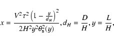
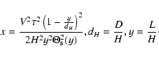
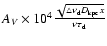
Ramani et al. (1986) and Blandford et al. (1986) have proposed the
Riss theory, which can be used to calculate the structure
functions of the normalized flux fluctuations of pulsars through
the interstellar medium. Blandford et al. (1986) assume that the
scattering density distribution of the extended medium is a
Gaussian:
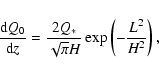 |
(1) |
where  is the total scattering strength of the extended
medium, H is the
is the total scattering strength of the extended
medium, H is the  width of the distribution and L is the distance to the observer.
It is also assumed that the spectrum of the electron density
fluctuations follows the isotropic power-law:
 |
(2) |
where
 is the spatial wave number of the fluctuation,
s is the spatial scale,
is the spatial wave number of the fluctuation,
s is the spatial scale,
 and
and
 are respectively
the inner and outer cutoffs of scale size. The indicator of the
rms of electron density fluctuations, CN2, characterizes
the strength of the scattering and is a function of location(z)
in the Galaxy. The value of the power-law index
are respectively
the inner and outer cutoffs of scale size. The indicator of the
rms of electron density fluctuations, CN2, characterizes
the strength of the scattering and is a function of location(z)
in the Galaxy. The value of the power-law index  ,
which is
in the range
,
which is
in the range
 ,
determines whether the scattering is
thought of as a turbulence spectrum (
,
determines whether the scattering is
thought of as a turbulence spectrum ( )
or a stochastic
superposition of discrete scattering structures (
)
or a stochastic
superposition of discrete scattering structures ( ).
Kolmogorov turbulence of the index
).
Kolmogorov turbulence of the index
 ,
is an
often-discussed model in the literature.
,
is an
often-discussed model in the literature.
The power spectrum of the phase fluctuations of the wavefronts is
also the power-law:
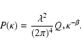 |
(3) |
The autocorrelation function F( )
and the structure
function D()
can be written as:
)
and the structure
function D()
can be written as:
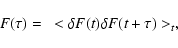 |
(4) |
![$\displaystyle D(\tau)=2\times[F(0)-F(\tau)]=2\times\left[<\delta F(t)\delta
F(t)>_{t}-<\delta F(t)\delta F(t+\tau)>_{t}\right],$](/articles/aa/full/2003/21/aa2778/img19.gif) |
|
|
(5) |
where  F(t) represents the normalized flux density fluctuation,
is the time lag and the subscript t means averaging over
all t.
F(t) represents the normalized flux density fluctuation,
is the time lag and the subscript t means averaging over
all t.
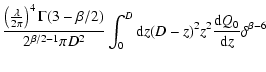
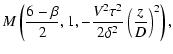
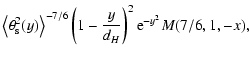
The autocorrelation function can be deduced from RISS theory as
(Qian 1995):
where M is the confluent hypergeometric function, D is the
distance of the source, V is the transverse velocity of the
source relative to the observer,  is the Gamma function,
 is the observation wavelength,
 ,
and
,
and
 is the apparent
angular radius of the source at the distance L.
is the apparent
angular radius of the source at the distance L.
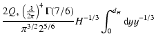
For
(Kolmogorov spectrum), the autocorrelation
function is (Qian 1995):
 |
(8) |
and for  ,
,
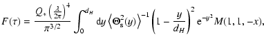 |
|
|
(9) |
 |
(10) |
Both the total scattering strength
and the scattering
angular radius
depend on the spectrum index and could
be obtained as (Romani et al. 1986):
(1)
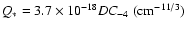 ,
,
 ,
,
(2)
 ,
,
 ,
where D and
are, respectively, in units of kpc
and m and
,
where D and
are, respectively, in units of kpc
and m and
 .
.
Stinebring et al. (2000) plotted the structure functions of the
unsmoothed flux density time series for 21 pulsars, of which two
pulsars' flux density structure functions do not have
well-characterized slopes and that of thirteen pulsars have a
single slope. However, for the remaining six pulsars, there is a
change in the slope of the flux density structure function,
corresponding to a change in the slope of the electron density
fluctuation spectrum at a spatial scale of about 1013 cm. In
this paper, the flux density structure functions of four pulsars,
PSRs B1642-03, B0329+54, B0736-40 and B0740-28, have been selected
to study because each of them has a apparent saturation region and
a single slope.
We use the Eqs. (7)-(10) of the RISS model given above to
calculate the structure function  ,
which have five
parameters:
,
which have five
parameters:
 and C-4.
The pulsar distance can be obtained from the association with
supernova remnants, interferometric measurements of annual
parallax, H I absorption measurements and dispersion measurements.
Lyne et al. (1985) concluded that the typical errors of distance
estimates were generally factors of 1.5-2. Now the electron
density model of Taylor & Cordes (1993, hereafter TC93) has been
widely used to obtain the pulsar distance from DM measurements,
which gives errors of about 25% for most pulsars. In the latest
electron density model, Cordes & Lazio (2002, hereafter NE2001)
made a few important revisions of TC93 model. In this paper, the
pulsar distances are taken from S2000, where the distances of PSR B0329+54 and PSR B0740-28 are derived from DM measurements from
the TC93 model, while for the other two pulsars, PSR B1642-03 and
PSR B0736-40, the distances are available from H I absorption
measurements (Frail & Weisberg 1990, hereafter FW90) and the
distance errors could be better or worse than 25%, depending on
the quality of the data. The distances adopted above for the four
pulsars are closer to those from NE2001.
The velocity is also an important observational parameter. There
are three main methods to estimate the space velocities of radio
pulsars. Pulsar proper motion velocity can be obtained from timing
and the interferometric measurements (e.g. Harrison et al. 1993).
The transverse speed can also be estimated from the interstellar
scintillation measurement. The scintillation velocity represents
the transverse velocity relative to the Earth and the scattering
screen, namely
 ,
where
,
where
 and
and
 are the proper motion velocity, the
velocity of the scattering screen and that of the Earth
respectively. Statistically, the earth motion causes a bias in the
scintillation speed that is about 30 km
are the proper motion velocity, the
velocity of the scattering screen and that of the Earth
respectively. Statistically, the earth motion causes a bias in the
scintillation speed that is about 30 km
 ,
and the
bulk flow of the density irregularities in the ISM is less than 10 km
(Gupta et al. 1999a). The
,
and the
bulk flow of the density irregularities in the ISM is less than 10 km
(Gupta et al. 1999a). The
 is estimated as
 ,
where
is in km
,
,
where
is in km
,
 in MHz,
D in kpc,
in MHz,
D in kpc,  in GHz and
 in seconds,
 ,
,
 and
and
 are the distance from the observer to the screen and that
from the screen to the pulsar (for a screen placed midway between
the pulsar and the observer, x=1). The constant AV was
taken to be
are the distance from the observer to the screen and that
from the screen to the pulsar (for a screen placed midway between
the pulsar and the observer, x=1). The constant AV was
taken to be
 by Gupta et al. (1994) and refined
to be
by Gupta et al. (1994) and refined
to be
 by Cordes & Rickett (1998). It is known
that there is a good agreement between the scintillation velocity
and the proper motion velocity in terms of the scattering screen
locating midway between the observer and the pulsar (Gupta 1995),
therefore scintillation speeds are generally considered to be
useful indicators of a pulsar's proper motion speed (Bhat et al.
1999a).
by Cordes & Rickett (1998). It is known
that there is a good agreement between the scintillation velocity
and the proper motion velocity in terms of the scattering screen
locating midway between the observer and the pulsar (Gupta 1995),
therefore scintillation speeds are generally considered to be
useful indicators of a pulsar's proper motion speed (Bhat et al.
1999a).
The power-law index, ,
reflects the fundamental physical
information of the scattering medium. The Kolmogorov turbulence
(
)
is produced by a cascade of wave energy from the
outer scale to the inner scale cut-off; and the Super-Kolmogorov
spectrum with the steeper power-law index ()
results from
the random superposition of discontinuities of the medium, such as
a collection of the shock fronts (Rickett 1990). Both the case of
and
are adopted to calculate the flux
density structure functions for all the four pulsars.
![\begin{figure}
\par\includegraphics[width=8.8cm,clip]{2778.f1.EPS}\end{figure}](/articles/aa/full/2003/21/aa2778/Timg54.gif) |
Figure 1:
The theoretical structure functions and the comparison with
observations for PSR B1642-03. a) The case for the best fit
parameters: the solid and dashed lines represent the structure
functions for
and ,
respectively. b)
The case where C-4 is treated as free parameter: the dashed,
solid and dotted lines represent
C-4=2.1, 1.8 and 1.5
 ,
respectively. c) The case where H is treated
as free parameter: the dashed, solid and dotted lines represent
H=0.4, 0.25 and 0.2 kpc, respectively. (Note: Solid dots are
observational data from S2000. Solid lines
represent theoretical results by the adoption of the best parameters listed in Table 1.
Dashed and dotted lines show the influence of the variation of one parameter on the structure
function while the other four parameters kept constant from Table 1.) ,
respectively. c) The case where H is treated
as free parameter: the dashed, solid and dotted lines represent
H=0.4, 0.25 and 0.2 kpc, respectively. (Note: Solid dots are
observational data from S2000. Solid lines
represent theoretical results by the adoption of the best parameters listed in Table 1.
Dashed and dotted lines show the influence of the variation of one parameter on the structure
function while the other four parameters kept constant from Table 1.) |
| Open with DEXTER |
![\begin{figure}
\par\includegraphics[width=8.8cm,clip]{2778.f2.EPS} \end{figure}](/articles/aa/full/2003/21/aa2778/Timg55.gif) |
Figure 2:
The theoretical structure functions and the comparison with observations
for PSR B0329+54.
a) The case for the best fit parameters: the solid and dashed lines represent the
structure functions for
and ,
respectively. b) The case where C-4 is
treated as free parameter: The dashed, solid and dotted lines
represent
C-4=1.5, 0.8 and 0.1
,
respectively. c) The case where H is treated as free
parameter: the dashed, solid and dotted lines represent H=1.2,
0.7 and 0.2 kpc, respectively. See the note of caption to Fig. 1
for details. |
| Open with DEXTER |
![\begin{figure}
\par\includegraphics[width=8.8cm,clip]{2778.f3.EPS} \end{figure}](/articles/aa/full/2003/21/aa2778/Timg56.gif) |
Figure 3:
The theoretical structure functions and the comparison with observations for PSR B0736-40.
a) The case for best fit parameters: the solid and dashed lines represent the
structure functions for
and ,
respectively. b) The case where C-4 is
treated as free parameter: the dashed, solid and dotted lines
represent
C-4=104.2, 104.1 and 104
,
respectively. c) The case where H is treated
as free parameter: the dashed, solid and dotted lines represent
H=1.5, 1.05 and 0.5 kpc respectively. See the note of caption to
Fig. 1 for details. |
| Open with DEXTER |
In our calculation, the distance (D) and the velocity (V) are
two physical parameters, while the other three parameters (
 and H) are considered to be free. In this paper,
and
both have been taken for calculation
for each pulsar.
and H) are considered to be free. In this paper,
and
both have been taken for calculation
for each pulsar.
The theoretically calculated structure functions (the solid lines)
and their comparison with the observational data of S2000 (the
solid dots) are presented in Figs. 1-4.
Table 1:
The best parameter values for theoretical
results and the comparison with some observational ones
from S2000.
There are three important quantities of the structure functions to
characterize the properties of pulsar flux density variation:
 and p. The modulation index m denotes the
amplitude of the flux density fluctuations and is defined as
and p. The modulation index m denotes the
amplitude of the flux density fluctuations and is defined as
 ,
where
,
where
 is the saturation
value.
is the saturation
value.
 is the value of the scintillation
timescale, the time lag at which the structure function reaches
half its saturation value. p is the logarithmic slope of the
structure function, which is related to the spectrum of electron
density fluctuations in ISM and the distribution along the line of
sight. The relation of
is the value of the scintillation
timescale, the time lag at which the structure function reaches
half its saturation value. p is the logarithmic slope of the
structure function, which is related to the spectrum of electron
density fluctuations in ISM and the distribution along the line of
sight. The relation of
 is used to
calculate p.
is used to
calculate p.
It is practical to obtain a set of the reasonable parameters in
terms of the treatments above, which will be described in detail
with respect to the pulsar PSR B1642-03.
The pulsar distance 0.5 kpc is derived from the H I absorption
measurements (FW 90) and the proper motion velocity 110 km
is given by Lyne et al. (1982). For the Kolmogorov
spectrum, the value C-4 can be determined due to the
relatively independent effects of C-4 and H on the
structure function. Such a property is shown clearly in Figs. 1b and 1c i.e., the saturation value (viz. modulation index) is
predominantly controlled by the value C-4, while not
influenced by the value of H, thereby the observed modulation
index within the error domain can give a strict restriction on the
possible range of C-4 and the best fitted value 1.8
is obtained. Then, the timescale depends only on the
value of H, and a value of H between 0.25 kpc and 0.4 kpc can
lead to theoretical curves being consistent with observations
(Fig. 1c). As Bhat et al. (1999a) mentioned, the scattering screen
is generally placed midway between the observer and the pulsar,
therefore we adopt H=0.25 kpc.
However, for the Super-Kolmogorov spectrum, the theoretical curve
will always be deviated from the observation no matter how the
other four parameters are adjusted. Thus we can conclude that
along the line of sight to this pulsar, the spectrum of the
electron density fluctuations corresponds to the Kolmogorov form,
but not the Super-Kolmogorov form, which is different from S2000.
In this way, the theoretical structure function curve is obtained
(the solid lines in Fig. 1) and a reasonable set of parameters
that best match the observational data is also determined as:
D=0.5 kpc, V=110 km
,
,
C-4=1.8
,
H=0.25 kpc.
Considering D and V as constant, in order to analyze how the
flux density structure functions are influenced by the variations
of the three free parameters ,
C-4 and H, each time
we make one of them variable and keep the other two constant in
each panel of Fig. 1.
Figure 1b displays the influence of C-4 on the structure
function.
C-4=1.5, 1.8 and 2.1
are chosen
for calculation and the structure function curve will move
parallel and downwards with C-4 increasing, which suggests
that the logarithmic slope of the structure function is
insensitive to the parameter C-4. Moreover, the modulation
index will become smaller and the timescale will be longer if
C-4 increases. The best fitted value 1.8
for C-4 is much smaller than the observational value 20
.
Such a discrepancy, also seen in pulsar PSR B0329+54,
can be interpreted by three possibilities. First, it is partially
because of measurement uncertainties in scattering strength.
Second, part of this discrepancy is to do with the fact that the
adopted distance may be significantly offset from the real value.
The third likely explanation is that the observational values of
scattering strength are obtained from the dynamic spectrum due to
DISS, while the fitted values are obtained by calculating the
structure function with the RISS theory. It may suggest that the
interstellar mediums causing DISS and RISS respectively probably
lie in different regions and have different spatial scales that
possibly bring different scattering strength.
For the sensitivity of the structure function to the value of H,
Fig. 1c shows that the structure function does not change
remarkably with the variation of H if H>D/2. However, when
H<D/2, the timescale will become slightly shorter with Hdecreasing, while m and p will not change.
Furthermore, we find that the flux density structure functions of
the other three pulsars are under a similar influence of the
variations of the free parameters, therefore a similar calculation
procedure has been carried out for each of them for the Kolmogorov
spectrum.
![\begin{figure}
\par\includegraphics[width=8.8cm,clip]{2778.f4.EPS} \end{figure}](/articles/aa/full/2003/21/aa2778/Timg71.gif) |
Figure 4:
The theoretical structure functions and the comparison with observations for PSR B0740-28.
a) The case for best fit parameters: the solid and dashed lines
represent the structure functions for
and ,
respectively. b) The case where C-4 is treated as free
parameter: the dashed, solid and dotted lines represent
C-4=200, 100 and 10
,
respectively. c)
The case where H is treated as free parameter: the dashed, solid
and dotted lines represent H=1.5, 0.95 and 0.5 kpc,
respectively. See the note of caption to Fig. 1 for details. |
| Open with DEXTER |
The best sets of five parameter values used to calculate the
theoretical flux density structure functions and some of the
observational ones from S2000 for comparison are listed in Table 1, where the distances and the proper motion velocities are taken
from S2000,
 is the best satisfied velocity in the
theoretical calculations and C-4 has two values, the
theoretical fit results and the observed values (calculated by
)
from DISS measurements
(S2000). The theoretical and observational values of
and p are listed in Table 2, where subscripts
"t'' and "o'' represent the theoretical and the
observational values, respectively.
is the best satisfied velocity in the
theoretical calculations and C-4 has two values, the
theoretical fit results and the observed values (calculated by
)
from DISS measurements
(S2000). The theoretical and observational values of
and p are listed in Table 2, where subscripts
"t'' and "o'' represent the theoretical and the
observational values, respectively.
Table 2:
The theoretical
and observational values of modulation indices,
logarithmic slopes and refractive timescales.
Along the line of sight to this pulsar, the spectrum of electron
density fluctuations is still uncertain. According to S2000, it is
either a Kolmogorov or Super-Kolmogorov spectrum. Our calculation
is mainly to examine the nature of the electron density
fluctuation spectrum.
For ,
like in the situation of PSR B1642-03, the
theoretical curve will always depart very far from observations no
matter how the other parameters are modulated, so the case of
can be ruled out.
For
,
by comparing the theoretical modulation index
with the observational value 0.37, a value of 0.8
for C-4 is best fitted, which is smaller than the
observational value 4
.
The best fit value
H=0.7 kpc (D/2) means that the scattering screen is located
midway between the observer and the pulsar, which agrees with Bhat
et al. (1999a).
The distance 1.4 kpc derived from the TC93 model is taken for
calculation. However, as for the velocity, it can be obtained from
many different measurements. Gupta (1995) gave the scintillation
velocity and the proper motion velocity, 126 km
and
145 km
,
respectively. Later on, the proper motions
of pulsars were improved by Fomalont et al. (1997) with VLA
observations and they figured out the transverse velocity of
 km
according to their measurements.
There is not much discrepancy among these velocity values.
However, with the observational parameters of S2000 and the
refined constant AV in the scintillation velocity calculation
formula given by Cordes & Rickett (1998), a smaller scintillation
velocity of 83 km
is obtained. It is found that
either the transverse velocity 135 km
or the
scintillation velocity 126 km
makes the theoretical
curve approximate to the observation, but can't result in the
allowable theoretical curve within the range of observational
error and the timescale is too much smaller than the observational
value. However, the adoption of 83 km
can give a
better match with observations. It may indicate that for this
pulsar the scintillation velocity is substantially smaller than
the proper motion velocity, as mentioned by Gupta et al. (1994).
The likely interpretation is that the bulk flow of the medium and
the orbital motion of the Earth also play important roles in
determining timescales (Bhat et al. 1998). Figure 2a shows that the
electron density fluctuation spectrum is much closer to the
Kolmogorov form than to the Super-Kolmogorov form along the line
of sight to this pulsar. We find that the agreement is better for
even lower values of velocity.
km
according to their measurements.
There is not much discrepancy among these velocity values.
However, with the observational parameters of S2000 and the
refined constant AV in the scintillation velocity calculation
formula given by Cordes & Rickett (1998), a smaller scintillation
velocity of 83 km
is obtained. It is found that
either the transverse velocity 135 km
or the
scintillation velocity 126 km
makes the theoretical
curve approximate to the observation, but can't result in the
allowable theoretical curve within the range of observational
error and the timescale is too much smaller than the observational
value. However, the adoption of 83 km
can give a
better match with observations. It may indicate that for this
pulsar the scintillation velocity is substantially smaller than
the proper motion velocity, as mentioned by Gupta et al. (1994).
The likely interpretation is that the bulk flow of the medium and
the orbital motion of the Earth also play important roles in
determining timescales (Bhat et al. 1998). Figure 2a shows that the
electron density fluctuation spectrum is much closer to the
Kolmogorov form than to the Super-Kolmogorov form along the line
of sight to this pulsar. We find that the agreement is better for
even lower values of velocity.
The cases of pulsars PSR B0736-40 and PSR B0740-28 are very
similar in terms of the adoption of parameters and the theoretical
results. For PSR B0736-40, the distance value 2.1 kpc is derived
from H I absorption measurements (FW90) and the proper motion
velocity 770 km
is calculated from proper motion
measurements by Fomalont et al. (1992). For PSR B0740-28, the
distance value 1.9 kpc is converted from DM using the TC93 model
and the proper motion velocity 240 km
is from the
proper motion measurements by Bailes et al. (1992). For the
Kolmogorov spectrum, the theoretical results are in good agreement
with observations. The best fitted values of C-4 are equal to
the observational values of DISS measurements from S2000. The best
fitted values of H are 1.05 kpc and 0.95 kpc, respectively,
showing that the scattering screen is placed midway between the
pulsar and the observer, which also agrees with Bhat et al.
(1999a).
The theoretical curves for ,
however, deviate very far
from observations no matter how the parameters are adjusted.
Therefore, the spectra of the electron density fluctuations fit
the Kolmogorov spectrum, but not the Super-Kolmogorov spectrum. It
confirms the conclusion of S2000 with respect to the nature of the
electron density fluctuation spectra along the lines of sights to
the two pulsars.
The effects of the parameter variations on the structure functions
(from Figs. 3 and 4) for these two pulsars are the same as
that for pulsars PSR B1642-03 and PSR B0329+54.
Although the distance and velocity are regarded as certain values
in the calculation above, in order to investigate the influence of
their uncertainties on structure functions, we modulate them
within the reasonable ranges to obtain the corresponding structure
functions.
The distances are made variable within the typical error range at
about 25% to calculate the structure function. Although the
modulation indices and the timescales can be slightly changed by
the variations of distance, the distance uncertainties generally
have no significant influence on structure functions. Therefore,
the effects of distance errors on the structure function can be
negligible.
Since the maximum error in estimating a pulsar's speed is  30 km
(Cordes 1986), the velocities are modulated in
range of 30 km
to calculate the structure
functions. For PSRs B1642-03, B0736-40 and B0740-28, the intensity
structure functions do not change with the velocity variations.
The larger uncertainties in the best fitted velocity for PSR B0329+54 may be due to the comparatively larger errors of the
structure function values at lower lags.
30 km
(Cordes 1986), the velocities are modulated in
range of 30 km
to calculate the structure
functions. For PSRs B1642-03, B0736-40 and B0740-28, the intensity
structure functions do not change with the velocity variations.
The larger uncertainties in the best fitted velocity for PSR B0329+54 may be due to the comparatively larger errors of the
structure function values at lower lags.
The theoretical flux density structure functions and the most
reasonable parameters for these four pulsars are obtained by means
of the RISS theory. The theoretical values of modulation indices,
logarithmic slopes and the timescales are also calculated and
compared with the observational values. From the theoretical
results, the electron density fluctuation spectra along the lines
of sight to these four pulsars are all consistent with the
Kolmogorov spectra. For the Super-Kolmogorov spectrum, the
theoretical curves will always deviate very far from observations
no matter how the parameters are adjusted. The modulation indices
are comparatively less prone to the location of the scattering
screen but critically depend on the scattering strength.
Therefore, the modulation index is a good indicator of scattering
strength and the former will become smaller with an increase of
the latter. For all the four pulsars, the scattering screen
located midway between the pulsar and the observer is reasonable,
which means H=D/2. The measurement uncertainties of distance and
velocity generally have no remarkable influence on structure
functions. Our results suggest that the long-term flux density
variations observed for these four pulsars are due to a
propagation effect (refractive scintillation), but not the
intrinsic variability.
Acknowledgements
We wish to thank Professors S. J. Qian and C. M. Zhang for their
helpful discussions. We also thank Professor A. G. Lyne for his
useful comments and profitable suggestions about our manuscript.
This work is supported by the National Natural Science Foundation
of China under Grant 10073001.
- Armstrong, J. W., Rickett, B. J., & Spangler, S. R. 1995, ApJ, 443, 209
In the text
NASA ADS
- Bailes, M., Manchester, R. N., Kesteven, M. J., Norris, R. P., & Reynolds, J. E. 1990, MNRAS, 247, 322
NASA ADS
- Bhat, N. D. R., Rao, A. P., & Gupta, Y. 1999a, ApJ, 121, 483
In the text
- Bhat, N. D. R., Gupta, Y., & Rao, A. P. 1999b, ApJ, 514, 249
In the text
NASA ADS
- Bhat, N. D. R., Rao, A. P., & Gupta, Y. 1999c, ApJ, 514, 272
In the text
NASA ADS
- Bhat, N. D. R., Gupta, Y., & Rao, A. P. 1998, ApJ, 500, 262
In the text
NASA ADS
- Bhat, N. D. R., & Gupta, Y. 2002, ApJ, 567, 342
In the text
NASA ADS
- Blandford, R., Narayan, R., & Romani, R. W. 1986, ApJ, 301, L53
In the text
NASA ADS
- Cordes, J. M., & Lazio, T. J. W. 2002 [astro-ph/0207156] (NE2001)
In the text
- Cordes, J. M., Piderbetsky, A., & Lovelace, R. V. E. 1986, ApJ, 310, 737
In the text
NASA ADS
- Cordes, J. M., & Rickett, B. J. 1998, ApJ, 507, 846
In the text
NASA ADS
- Esamdin, A., Wu, X. J., & Zhang, J. 2000, ChA&A, 24, 275
In the text
NASA ADS
- Frail, D. A., & Weisberg, J. M. 1990, AJ, 100, 743 (FW90)
In the text
NASA ADS
- Fomalont, E. B., Goss, W. M., Lyne, A. G., Manchester, R. N., & Justtanont, K. 1992, MNRAS, 258, 497
In the text
NASA ADS
- Fomalont, E. B., Goss, W. M., Manchester, R. N., & Lyne, A. G. 1997, MNRAS, 286, 82
In the text
- Gupta, Y., Rickett, B. J., & Coles, W. A. 1993, ApJ, 403, 183
In the text
NASA ADS
- Gupta, Y., Rickett, B. J., & Lyne, A. G. 1994, MNRAS, 269, 1035
In the text
NASA ADS
- Gupta, Y. 1995, ApJ, 451, 717
In the text
NASA ADS
- Harrison, P. A., Lyne, A. G., & Anderson, B. 1993, MNRAS, 261, 113
In the text
NASA ADS
- Hewish, A., Bell, S. J., Pilkington, J. D. H., Scott, P. F., & Collins, R. A. 1968, Nature, 217, 709
In the text
- Kaspi, V., & Stinebring, D. 1992, ApJ, 392, 530
In the text
NASA ADS
- LaBrecque, D. R., Rankin, J. M., & Cordes, J. M. 1994, AJ, 108, 1854
In the text
NASA ADS
- Lyne, A. G., Anderson, B., & Salter, M. J. 1982, MNRAS, 201, 503
In the text
NASA ADS
- Lyne, A. G., Manchester, R. N., & Taylor, J. H. 1985, MNRAS, 213, 613
In the text
NASA ADS
- Qian, S. J. 1995, ChA&A, 19, 523
In the text
NASA ADS
- Rickett, B. J. 1990, ARA&A, 28, 561
In the text
NASA ADS
- Rickett, B. J., Coles, W. A., & Bourgois, G. 1984, A&A, 134, 390
In the text
NASA ADS
- Rickett, B. J., & Lyne, A. G. 1990, MNRAS, 244, 68
NASA ADS
- Romani, R. W., Narayan, R., & Blandford, R. 1986, MNRAS, 220, 19
In the text
NASA ADS
- Sieber, W. 1982, A&A, 113, 311
In the text
NASA ADS
- Stinebring, D. R., & Condon, J. J. 1990, ApJ, 352, 207
In the text
NASA ADS
- Stinebring, D. R., Faison, M. D., & Mckinnon, M. M. 1996, ApJ, 460, 460
In the text
NASA ADS
- Stinebring, D. R., Smirnova, T. V., & Hankins, T. H., et al. 2000, ApJ, 539, 300 (S2000)
In the text
NASA ADS
- Taylor, J. H., & Cordes, J. M. 1993, ApJ, 411, 674 (TC93)
In the text
NASA ADS
- Wang, N., Wu, X. J., & Manchester, R. N., et al. 2001, ChJAA, 1, 430
In the text
- Wu, X. J., & Chian, A. C. L. 1995, ApJ, 443, 261
In the text
NASA ADS
Copyright ESO 2003
![\begin{figure}
\par\includegraphics[width=8.8cm,clip]{2778.f1.EPS}\end{figure}](/articles/aa/full/2003/21/aa2778/img54.gif)
![\begin{figure}
\par\includegraphics[width=8.8cm,clip]{2778.f2.EPS} \end{figure}](/articles/aa/full/2003/21/aa2778/img55.gif)
![\begin{figure}
\par\includegraphics[width=8.8cm,clip]{2778.f3.EPS} \end{figure}](/articles/aa/full/2003/21/aa2778/img56.gif)
![\begin{figure}
\par\includegraphics[width=8.8cm,clip]{2778.f4.EPS} \end{figure}](/articles/aa/full/2003/21/aa2778/img71.gif)